Generalized Nonlinear Robust Energy-to-Peak Filtering for Differential Algebraic Systems

Abstract

The problem of robust nonlinear energy-to-peak filtering for nonlinear descriptor systems with model uncertainties is addressed. The system is assumed to have nonlinearities both in the state and output equations as well as norm-bounded time-varying uncertainties in the realization matrices. A generalized nonlinear dynamic filtering structure is proposed for such a class of systems with more degrees of freedom than the conventional static-gain and dynamic filtering structures. The $\mathcal{L}_{2}-\mathcal{L}_{\infty}$ filter is synthesized through semidefinite programming and strict LMIs, in which the energy-to-peak filtering performance in optimized.

keywords: Robust Filtering, Energy-to-Peak Filtering, Nonlinear $\mathcal{L}_{2}-\mathcal{L}_{\infty}$, Descriptor Systems, Semidefinite Programming, Lipschitz Systems, DAE

I Introduction

Descriptor systems, also referred to as singular systems or differential-algebraic equation (DAE) systems, arise from an inherent and natural modeling approach, and have vast applications in engineering disciplines such as power systems, network and circuit analysis, and multibody mechanical systems, as well as in social and economic sciences. Generalizing the regular state space modeling (i.e. pure ODE systems), descriptor systems can characterize a larger class of systems than conventional state space models and can describe the physics of the system more precisely. Many approaches have been developed to design state observers for descriptor systems. Observer design and filtering of nonlinear dynamic systems has been a subject of extensive research in the last decade due to its theoretical and practical importance. In [7, 6, 16, 8, 9, 28, 20, 14, 21, 26, 32] various methods of observer design for linear and nonlinear descriptor systems have been proposed. In [6] an observer design procedure is proposed for a class nonlinear descriptor systems using an appropriate coordinate transformation. In [26], the authors address the unknown input observer design problem dividing the system into two dynamic and static subsystems. Reference [20] studies the full order and reduced order observer design for Lipschitz nonlinear Systems.

A fundamental limitation encountered in conventional observer theory is that it can not guarantee observer performance in the presence of model uncertainties and/or disturbances and measurement noise. One of the most popular ways to deal with the nonlinear state estimation problem is the extended Kalman filtering. However, the requirements of specific noise statistics and weakly nonlinear dynamics, has restricted its applicability to nonlinear systems. To deal with the nonlinear filtering problem in the presence of model uncertainties and unknown exogenous disturbances, we can resort the robust $H_{\infty}$ filtering, and $\mathcal{L}_{2}-\mathcal{L}_{\infty}$ filtering approaches. See for example [10, 29, 22, 23, 25, 1, 3, 4, 2, 5] and the references therein. The mathematical system model is assumed to be affected by time-varying parametric uncertainties, while norm bounded disturbances affect the measurements. Each of the two criteria has its own physical implications and applications. In $H_{\infty}$ filtering, the $\mathcal{L}_{2}$ gain from the exogenous disturbance to the filter error is guaranteed to be less than a prespecified level. Therefore, this $\mathcal{L}_{2}$ gain minimization is in fact an energy-to-energy filtering problem. In $\mathcal{L}_{2}-\mathcal{L}_{\infty}$ filtering, the ratio of the peak value of the error ($\mathcal{L}_{\infty}$ norm) to the energy of disturbance ($\mathcal{L}_{2}$ norm) is considered, therefore, conforming an energy-to-peak performance. This strategy has been used for both full-order and reduced-order filter design through LMIs in [13, 11] and also as a way for model reduction in [12]. Recently, $\mathcal{L}_{2}-\mathcal{L}_{\infty}$ filtering has been addressed for linear descriptor systems [31, 30]. However, the problem of $\mathcal{L}_{2}-\mathcal{L}_{\infty}$ filtering for nonlinear descriptor systems has not been fully investigated yet, despite the practical motivation and the great importance.

In this paper, we study the robust nonlinear $\mathcal{L}_{2}-\mathcal{L}_{\infty}$ filtering for continuous-time Lipschitz descriptor systems in the presence of disturbance and model uncertainties, in the LMI optimization framework. We consider nonlinearities in both the state and output equations, Furthermore, we generalize the filter structure by proposing a general dynamical filtering framework that can easily capture both dynamic and static-gain filter structures as special cases. The proposed dynamical structure has additional degrees of freedom compared to conventional static-gain filters and consequently is capable of robustly stabilizing the filter error dynamics for systems for which an static-gain filter can not be found.

Stability of nonlinear ODE systems is established through Lyapunov theory, while the stability of DAE systems is established through LaSalle’s invariant set theory. The results on ODEs, such as in [22, 23, 25, 1, 3, 4], are directly cast into strict LMIs while the results here are a set of linear matrix equations and inequalities leading into a semidefinite programming. The developed SDP problem is then smartly converted into a strict LMI formulation, without any approximations, and is efficiently solvable by readily available LMI solvers.

The rest of the paper is organized as follows. In section II, the problem statement and some preliminaries are mentioned. In section III, we propose a new method for robust $\mathcal{L}_{2}-\mathcal{L}_{\infty}$ filter design for nonlinear descriptor uncertain systems based on semidefinite programming (SDP). In Section IV, the SDP problem of Section III is converted into strict LMIs. In section V, we show the proposed filter design procedure through an illustrative example.

II Preliminaries and Problem Statement

Consider the following class of continuous-time uncertain nonlinear descriptor systems:

$$\left(\Sigma_{s}\right):\mathbf{E}\dot{x}(t) =(A+\Delta A(t))x(t)+\Phi(x,u)+Bw(t)$$ (1)

$$y(t) =(C+\Delta C(t))x(t)+\Psi(x,u)+Dw(t)$$ (2)

where $x\in{\mathbb{R}}^{n},u\in{\mathbb{R}}^{m},y\in{\mathbb{R}}^{p}$ and $\Phi(x,u)$ and $\Psi(x,u)$ contain nonlinearities of second order or higher. $\mathbf{E}$, $A$, $B$, $C$ and $D$ are constant matrices with compatible dimensions; $\mathbf{E}$ may be singular. When the matrix $\mathbf{E}$ is singular, the above form is equivalent to a set of differential-algebraic equations (DAEs) [7]. In other words, the dynamics of descriptor systems, comprise a set of differential equations together with a set of algebraic constraints. Unlike conventional state space systems in which the initial conditions can be freely chosen in the operating region, in the descriptor systems, initial conditions must be consistent, i.e. they should satisfy the algebraic constraints. Consistent initialization of descriptor systems naturally happens in physical systems but should be taken into account when simulating such systems [24]. Without loss of generality, we assume that $0<rank(\mathbf{E})=s<n$; $x(0)=x_{0}$ is a consistent (unknown) set of initial conditions. If the matrix $\mathbf{E}$ is non-singular (i.e. full rank), then the descriptor form reduces to the conventional state space. The number of algebraic constraints that must be satisfied by $x_{0}$ equals $n-s$. We assume the pair $(\mathbf{E},A)$ to be regular, i.e. $\det(s\mathbf{E}-A)\neq 0$ for some $s\in\mathbb{C}$ and $(\mathbf{E},A,C)$ to be observable, i.e. [17]

$$rank\left[\begin{array}[]{c}s\mathbf{E}-A\\ C\\ \end{array}\right]=n,\ \forall\ s\in\mathbb{C}.$$ (5)

We also assume that the system (1)-(2) is locally Lipschitz with respect to $x$ in a region $\mathcal{D}$ containing the origin, uniformly in $u$, i.e.:

$$\Phi(0,u^{*})=\Psi(0,u^{*})=0,$$

$$\|\Phi(x_{1},u^{*})-\Phi(x_{2},u^{*})\|\leqslant\gamma_{1}\|x_{1}-x_{2}\|,\hskip 5.69054pt\forall\,x_{1},x_{2}\in\mathcal{D}$$

$$\|\Psi(x_{1},u^{*})-\Psi(x_{2},u^{*})\|\leqslant\gamma_{2}\|x_{1}-x_{2}\|,\hskip 5.69054pt\forall\,x_{1},x_{2}\in\mathcal{D}$$

where $\|.\|$ is the induced 2-norm, $u^{*}$ is any admissible control signal and $\gamma_{1},\ \gamma_{2}>0$ are the Lipschitz constants of $\Phi(x,u)$ and $\Psi(x,u)$, respectively. If the nonlinear functions $\Phi(x,u)$ and $\Psi(x,u)$ satisfy the Lipschitz continuity condition globally in $\mathbb{R}^{n}$, then the results will be valid globally. $w(t)\in\mathcal{L}_{2}[0,\infty)$ is an unknown exogenous disturbance, and $\Delta A(t)$ and $\Delta C(t)$ are unknown matrices representing time-varying parameter uncertainties, and are assumed to be of the form

$$\left[\begin{array}[]{c}\Delta A(t)\\ \Delta C(t)\\ \end{array}\right]=\left[\begin{array}[]{c}M_{1}\\ M_{2}\\ \end{array}\right]F(t)N$$ (10)

where $M_{1}$, $M_{2}$ and $N$ are known real constant matrices and $F(t)$ is an unknown real-valued time-varying matrix satisfying

$$F^{T}(t)F(t)\leq I\hskip 28.45274pt\forall\ t\in[0,\infty).$$ (11)

The parameter uncertainty in the linear terms can be regarded as the variation of the operating point of the nonlinear system. It is also worth noting that the structure of parameter uncertainties in (10) has been widely used in the problems of robust control and robust filtering for both continuous-time and discrete-time systems and can capture the uncertainty in a number of practical situations [10], [18].

II-A Filter Structure

We propose the general filtering framework of the following form

$$\begin{split}\left(\Sigma_{o}\right):\mathbf{E}\dot{x}_{F}(t)&=A_{F}x_{F}(t)+B_{F}y(t)+\mathcal{E}_{1}\Phi(x_{F},u)+\mathcal{E}_{2}\Psi(x_{F},u)\\ z_{F}(t)&=C_{F}x_{F}(t)+\mathcal{E}_{3}\Psi(x_{F},u).\end{split}$$ (12)

The proposed framework can capture both dynamic and static-gain filter structures by proper selection of $\mathcal{E}_{1}$, $\mathcal{E}_{2}$ and $\mathcal{E}_{3}$. Choosing $\mathcal{E}_{1}=I$, $\mathcal{E}_{2}=0$ and $\mathcal{E}_{3}=0$ leads to the following dynamic filter structure:

$$\begin{split}\mathbf{E}\dot{x}_{F}(t)&=A_{F}x_{F}(t)+B_{F}y(t)+\Phi(x_{F},u)\\ z_{F}(t)&=C_{F}x_{F}(t).\end{split}$$ (13)

Furthermore, for the static-gain filter structure we have:

$$\begin{split}\mathbf{E}\dot{x}_{F}(t)&=Ax_{F}(t)+\Phi(x_{F},u)+L[y(t)-Cx_{F}(t)-\Psi(x_{F},u)]\\ z_{F}(t)&=x_{F}(t).\end{split}$$ (14)

Hence, with $A_{F}=A-LC,\ B_{F}=L,\ C_{F}=I,\mathcal{E}_{1}=I,\ \mathcal{E}_{2}=-L,\ \mathcal{E}_{3}=0$, the general filter captures the well-known static-gain observer filter structure as a special case. We prove our result for the general filter of class $(\Sigma_{o})$.

Now, suppose $z(t)=Hx(t)$ stands for the controlled output for states to be estimated where $H$ is a known matrix. The estimation error is defined as

$$e(t)\triangleq z(t)-z_{F}(t)=-C_{F}x_{F}+(H-C)x-\mathcal{E}_{3}\Psi(x_{F},u).$$ (15)

The filter error dynamics is given by

$$\left(\Sigma_{e}\right):\mathbf{\widetilde{E}}\dot{\xi}(t) =(\widetilde{A}+\Delta\widetilde{A})\xi(t)+S_{1}\Omega(\xi,u)+\widetilde{B}w(t)$$ (16)

$$e(t) =\widetilde{C}\xi(t)+S_{2}\Omega(\xi,u),$$ (17)

where,

$$\xi\triangleq\left[\begin{array}[]{c}x_{F}\\ x\\ \end{array}\right],\widetilde{A}=\left[\begin{array}[]{cc}A_{F}&B_{F}C\\ 0&A\\ \end{array}\right],\Delta\widetilde{A}=\left[\begin{array}[]{cc}0&B_{F}\Delta C\\ 0&\Delta A\\ \end{array}\right]$$ (24)

$$\mathbf{\widetilde{E}}=\left[\begin{array}[]{cc}\mathbf{E}&0\\ 0&\mathbf{E}\\ \end{array}\right],\widetilde{B}=\left[\begin{array}[]{c}B_{F}D\\ B\\ \end{array}\right],\widetilde{C}=\left[\begin{array}[]{cc}-C_{F}&H\\ \end{array}\right],$$ (30)

$$\Omega(\xi,u)=\left[\begin{array}[]{cccc}\Phi(x,u)&\Psi(x,u)&\Phi(x_{F},u)&\Psi(x_{F},u)\end{array}\right]^{T}$$ (32)

$$S_{1}=\left[\begin{array}[]{cccc}0&B_{F}&\mathcal{E}_{1}&\mathcal{E}_{2}\\ I&0&0&0\\ \end{array}\right],S_{2}=\left[\begin{array}[]{cccc}0&0&0&-\mathcal{E}_{3}\\ \end{array}\right].$$ (36)

For the nonlinear function $\Omega$, it is easy to show that

$$\Gamma\triangleq\left[\begin{array}[]{cccc}0&0&\gamma_{1}&\gamma_{2}\\ \gamma_{1}&\gamma_{2}&0&0\\ \end{array}\right]^{T},\ \|\Gamma\|\ =\sqrt{\gamma_{1}^{2}+\gamma_{2}^{2}}$$ (39)

$$\|\Omega(\xi_{1},u)-\Omega(\xi_{2},u)\|\leq\|\Gamma(\xi_{1}-\xi_{2})\|=\sqrt{\gamma_{1}^{2}+\gamma_{2}^{2}}\|\xi_{1}-\xi_{2}\|\triangleq\gamma\|\xi_{1}-\xi_{2}\|.$$ (40)

Thus, the filter error system is Lipschitz with Lipschitz constant $\gamma$.

II-B Disturbance Attenuation Level

Our purpose is to design the filter matrices $A_{F}$, $B_{F}$ and $C_{F}$, such that in the absence of disturbance, the filter error dynamics is asymptotically stable and moreover, for all $w(t)\in\mathcal{L}_{2}[0,\infty)$, subject to zero error initial conditions, the following $\mathcal{L}_{2}-\mathcal{L}_{\infty}$ norm upper bound is simultaneously guaranteed.

$$\|e\|_{\infty}\leq\mu\|w\|_{2},$$ (41)

where $\|.\|_{\infty}$ and $\|.\|_{2}$ denote the signal $2-norm$ and $infinity-norm$, respectively, defined as:

$$\|w(t)\|_{2} =\sqrt{\int^{\infty}_{0}\left(w^{T}(t)w(t)\right)dt}$$

$$\|e(t)\|_{\infty} =\sup_{t}\sqrt{|e(t)|^{2}}\ \ \ \forall\ t\in[0,\infty).$$

In the following, we mention some useful lemmas that will be used later in the proof of our results.

Lemma 1. [29] For any $x,y\in\mathbb{R}^{n}$ and any positive definite matrix $P\in\mathbb{R}^{n\times{n}}$, we have

$$2x^{T}y\leq x^{T}Px+y^{T}P^{-1}y.$$

Lemma 2. [29] Let $A,D,E,F$ and P be real matrices of appropriate dimensions with $P>0$ and $F$ satisfying $F^{T}F\leq I$. Then for any scalar $\epsilon>0$ satisfying $P^{-1}-\epsilon^{-1}DD^{T}>0$, we have

$$(A+DFE)^{T}P(A+DFE)\leq A^{T}(P^{-1}-\epsilon^{-1}DD^{T})^{-1}A+\epsilon E^{T}E.$$

Lemma 3. [15, p. 301] A matrix $A\in\mathbb{R}^{n\times n}$ is invertible if there is a matrix norm $\||.\||$ such that $\||I-A\||<1$.

III $\mathcal{L}_{2}-\mathcal{L}_{\infty}$ Filter Synthesis

In this section, a generalized dynamic $\mathcal{L}_{2}-\mathcal{L}_{\infty}$ filtering method with guaranteed disturbance attenuation level $\mu$ is proposed.

Theorem 1. Consider the Lipschitz nonlinear system $\left(\Sigma_{s}\right)$ along with the general filter $\left(\Sigma_{o}\right)$. The filter error dynamics is (globally) asymptotically stable with an optimized $\mathcal{L}_{2}-\mathcal{L}_{\infty}(w\rightarrow e)$ gain, $\mu^{*}$, if there exists scalars $\zeta>0$, $\epsilon>0$ and $\alpha>0$, and matrices $C_{F}$, $P_{1}$, $P_{2}$, $G_{1}$, $G_{2}$ and $\mathcal{E}_{3}$, such that the following optimization problem has a solution.

$$\hskip 14.22636pt\min(\zeta)$$

$$\Xi_{1}=\left[\begin{array}[]{ccc}\Pi_{1}&\Pi_{2}&\Pi_{3}\\ \star&-\epsilon I&0\\ \star&\star&-\zeta I\\ \end{array}\right]<0$$ (45)

$$\Xi_{2}=\left[\begin{array}[]{ccccc}-\mathbf{E}^{T}P_{1}&C_{F}^{T}&\alpha\gamma I&-C_{F}^{T}H&0\\ \star&-\frac{1}{3}I&0&0&0\\ \star&\star&-\frac{1}{3}I&0&0\\ \star&\star&\star&\Lambda_{3}&\alpha\gamma I\\ \star&\star&\star&\star&-\frac{1}{3}I\\ \end{array}\right]<0$$ (51)

$$\Xi_{3}=\left[\begin{array}[]{cc}\alpha I&\mathcal{E}_{3}\\ \star&\alpha I\\ \end{array}\right]>0$$ (54)

$$\Xi_{4}=\left[\begin{array}[]{cc}I&I-P_{1}^{T}\\ \star&I\\ \end{array}\right]>0$$ (57)

$$\mathbf{E}^{T}P_{1}=P_{1}^{T}\mathbf{E}\geq 0$$ (58)

$$\mathbf{E}^{T}P_{2}=P_{2}^{T}\mathbf{E}\geq 0$$ (59)

where the elements of $\Xi_{1}$ and $\Xi_{2}$ are as defined in the following, $\Lambda_{1}=G_{1}+G_{1}^{T}+\gamma^{2}I$, $\Lambda_{2}=A^{T}P_{2}+P_{2}A+\gamma^{2}I+\epsilon N^{T}N$, $\Lambda_{3}=H^{T}H-\mathbf{E}^{T}P_{2}$,

$$\Pi_{1}=\left[\begin{array}[]{cc}\Lambda_{1}&G_{2}C\\ \star&\Lambda_{2}\\ \end{array}\right],\Pi_{2}=\left[\begin{array}[]{cc}0&G_{2}M_{2}\\ 0&P_{2}M_{1}\\ \end{array}\right],$$ (64)

$$\Pi_{3}=\left[\begin{array}[]{cccc}0&G_{2}&P_{1}\mathcal{E}_{1}&P_{1}\mathcal{E}_{2}\\ P_{2}&0&0&0\\ \end{array}\right].$$ (67)

Once the problem is solved:

$$A_{F} =P^{-1}_{1}G_{1},\ B_{F}=P^{-1}_{1}G_{2}$$ (68)

$$C_{F}\ \text{is directly obtained},\ \mu^{*}\triangleq\min(\mu)=\sqrt{\zeta^{*}}.$$

Proof: Consider the following Lyapunov function candidate

$$V(\xi(t))=\xi^{T}\mathbf{\widetilde{E}}^{T}P\xi.$$ (69)

To prove the stability of the filter error dynamics, we employ the well-established generalized Lyapunov stability theory as discussed in [14], [21] and [17] and the references therein. The generalized Lyapunov stability theory is mainly based on an extended version of the well-known LaSalle’s invariance principle for descriptor systems. Based on this theory, the above function along with the conditions (58) and (59) is a generalized Lyapunov function (GLF) for the system $\left(\Sigma_{e}\right)$ where $P=diag(P_{1},P_{2})$. In fact, it can be shown that $V(\xi(t))=0$ if and only if $\mathbf{\widetilde{E}}\xi=0$ and positive elsewhere [14, Ch. 2]. Now, we calculate the derivative of $V$ along the trajectories of $\left(\Sigma_{e}\right)$. We have

$$\dot{V} =\dot{\xi}^{T}\mathbf{\widetilde{E}}^{T}P\xi+\xi^{T}\mathbf{\widetilde{E}}^{T}P\dot{\xi}=2\xi^{T}(\widetilde{A}+\Delta\widetilde{A})^{T}P\xi+2\xi^{T}PS_{1}\Omega+2\xi^{T}P\widetilde{B}w.$$ (70)

Now, we define

$$J\triangleq V-\int^{\infty}_{0}\left(\mu^{2}w^{T}w\right)dt.$$ (71)

Therefore,

$$J<\int^{\infty}_{0}\left(\dot{V}-\mu^{2}w^{T}w\right)dt.$$ (72)

So a sufficient condition for $J\leq 0$ is that

$$\forall\ t\in[0,\infty),\hskip 14.22636pt\dot{V}-\mu^{2}w^{T}w\leq 0.$$ (73)

Thus, using Lemma 1,

$$\dot{V}-\mu^{2}w^{T}w\leq 2\xi^{T}(\widetilde{A}+\Delta\widetilde{A})^{T}P\xi+2\xi^{T}PS_{1}\Omega+2\xi^{T}P\widetilde{B}w-\mu^{2}w^{T}w$$

$$\leq \xi^{T}[2(\widetilde{A}+\Delta\widetilde{A})^{T}P+PS_{1}^{T}S_{1}P]\xi+2\xi^{T}P\widetilde{B}w+\Omega^{T}\Omega$$

$$\leq \xi^{T}[2(\widetilde{A}+\Delta\widetilde{A})^{T}P+PS_{1}^{T}S_{1}P]\xi+2\xi^{T}P\widetilde{B}w+\Omega^{T}\Omega-\mu^{2}w^{T}w.$$ (74)

Knowing that $\|\Omega(\xi)\|\leq\|\Gamma\xi\|$, we have,

$$\Omega^{T}\Omega\leq\gamma^{2}\xi^{T}\xi.$$ (75)

On the other hand,

$$\Delta\widetilde{A} =\left[\begin{array}[]{cc}0&B_{F}\Delta C\\ 0&\Delta A\\ \end{array}\right]=\left[\begin{array}[]{cc}0&B_{F}M_{2}FN\\ 0&M_{1}FN\\ \end{array}\right]=\left[\begin{array}[]{cc}0&B_{F}M_{2}\\ 0&M_{1}\\ \end{array}\right]F\left[\begin{array}[]{cc}0&0\\ 0&N\\ \end{array}\right]\triangleq\widetilde{M_{1}}F\widetilde{N}.$$ (84)

Therefore, based on (75) and using Lemma 2 we can write

$$\dot{V}-\mu^{2}w^{T}w<\xi^{T}[ \widetilde{A}^{T}P+P\widetilde{A}+\epsilon\widetilde{N}^{T}N+\epsilon_{1}^{-1}P\widetilde{M}_{1}\widetilde{M}_{1}P$$

$$+PS_{1}S_{1}^{T}P+\gamma^{2}]\xi+2\xi^{T}P\widetilde{B}w-\mu^{2}w^{T}w.$$ (85)

Now, a sufficient condition for (73) is that the right hand side of (85) be negative definite. Using Schur complements, this is equivalent to the following LMI. Note that having $w=0$, (70) is already included in (74) and consequently in (85).

$$\left[\begin{array}[]{cccc}\widetilde{A}^{T}P+P\widetilde{A}+\gamma^{2}I+\epsilon\widetilde{N}^{T}\widetilde{N}&P\widetilde{M}_{1}&PS_{1}&P\widetilde{B}\\ \star&-\epsilon I&0&0\\ \star&\star&-I&0\\ \star&\star&\star&-\zeta I\\ \end{array}\right]<0.$$ (90)

Substituting from (84), having $P=diag(P_{1},P_{2})$, defining change of variables $G_{1}\triangleq P_{1}A_{F}$, $G_{2}\triangleq P_{1}B_{F}$ and $\zeta=\mu^{2}$, and using Schur complements, the LMI (45) is obtained.
In the next step, we establish the inequality $e^{T}e<V$. We have $e^{T}e=\xi^{T}\widetilde{C}^{T}\widetilde{C}\xi+2\xi^{T}\widetilde{C}^{T}S_{2}\Omega+\Omega^{T}S_{2}^{T}S_{2}\Omega$. Therefore, $e^{T}e\leq 3\xi^{T}\widetilde{C}^{T}\widetilde{C}\xi+3\Omega^{T}S_{2}^{T}S_{2}\Omega$, while $\Omega^{T}S_{2}^{T}S_{2}\Omega\leq\|S_{2}^{T}S_{2}\|\Omega^{T}\Omega=\|\mathcal{E}_{3}^{T}\mathcal{E}_{3}\|\Omega^{T}\Omega$. Without loss of generality, we assume that there is a scalar $\alpha$ such that $\|\mathcal{E}_{3}\mathcal{E}_{3}^{T}\|<\alpha^{2}$ (i.e. $\|\mathcal{E}_{3}\|<\alpha$), where $\alpha>0$ is an unknown variable. Thus, we need to have $e^{T}e\leq 3\xi^{T}[\widetilde{C}^{T}\widetilde{C}+\alpha^{2}\gamma^{2}I]\xi<\xi^{T}\mathbf{\widetilde{E}}^{T}P\xi$, which by means of Schur complements is equivalent to the LMI (51). LMI (54) is equivalent to the condition $\|\mathcal{E}_{3}\|<\alpha_{1}$. So, based on the above, we have

$$\forall\ t\ \ e^{T}(t)e(t)\leq\mu^{2}\int^{\infty}_{0}\left(w^{T}(t)w(t)dt\right),$$

Therefore, $\|e(t)\|_{\infty}\leq\mu\|w(t)\|_{2}$. Note that neither $P_{1}$ nor $P_{2}$ are necessarily positive definite. However, in order to find $A_{F}$ and $B_{F}$ in (68), $P_{1}$ must be invertible. Since we are using the spectral matrix norm (matrix 2-norm) throughout this paper, based on Lemma 3, a sufficient condition for nonsingularity of $P_{1}$ is that $\|I-P_{1}\|=\sigma_{max}(I-P_{1})<1$. This is equivalent to $I-(I-P_{1})^{T}(I-P_{1})>0$. Thus, using Schur’s complement, LMI (57) guarantees the nonsingularity of $P_{1}$. $\blacksquare$

Remark 1. The proposed LMIs are linear in $\alpha$ and $\mu$. Thus, either can be a fixed constant or an optimization variable. Given this, it may be more realistic to have a combined performance index. This leads to a multiobjective convex optimization problem optimizing both $\alpha$ and $\mu$, simultaneously. See [1] and [4] for details and examples of multiobjective optimization approach to filtering for other classes of nonlinear systems.

Figure 1 shows a classification of the estate estimators in terms of their functionality, and the computational frameworks used. Next section will elaborate further on the differences between strict LMIs and semidefinite programming (SDP).

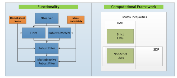
Figure 1: State estimation functionality and computational framework

Note that $\mathcal{E}_{1}$ and $\mathcal{E}_{2}$ are not optimization variables. They are apriory fixed constant matrices that determine the structure of the filter while $\mathcal{E}_{3}$ can be either a fixed gain or an optimization variable.

IV Converting SDP into strict LMIs

Due to the existence of equalities and non-strict inequalities in (58) and (59), the optimization problem of Theorem 1 is not a convex strict LMI Optimization and instead it is a Semidefinite Programming (SDP) with quasi-convex solution space. The SDP problem proposed in Theorem 1 can be solved using freely available packages such as YALMIP [19] or SeDuMi [27]. However, in order to use the numerically more efficient Matlab strict LMI solver, in this section we convert the SDP problem proposed in Theorem 1 into a strict LMI optimization problem through a smart transformation. We use a similar approach as used in [28] and [20]. Let $\mathbf{E}_{\bot}\in\mathbb{R}^{(n-s)\times n}$ be the orthogonal complement of $\mathbf{E}$ such that $\mathbf{E}_{\bot}\mathbf{E}=0$ and $\text{rank}(\mathbf{E}_{\bot})=n-s$. The following corollary gives the strict LMI formulation.

Corollary 1. Consider the Lipschitz nonlinear system $\left(\Sigma_{s}\right)$ along with the general filter $\left(\Sigma_{o}\right)$. The filter error dynamics is (globally) asymptotically stable with an optimized $\mathcal{L}_{2}-\mathcal{L}_{\infty}(w\rightarrow e)$ gain, $\mu^{*}$, if there exists a scalars $\zeta>0$, $\epsilon>0$ and $\alpha>0$, and matrices $C_{F}$, $X_{1}>0$, $X_{2}>0$, $Y_{1}$, $Y_{2}$, $G_{1}$, $G_{2}$ and $\mathcal{E}_{3}$ such that the following LMI optimization problem has a solution.

$$\hskip 8.5359pt\min(\zeta)$$

$$\Xi_{1}<0,\ \Xi_{2}>0,\ \Xi_{3}>0$$

$$\Xi_{4}=\left[\begin{array}[]{cc}I&I-P_{1}^{T}\\ \star&I\\ \end{array}\right]>0,$$ (93)

where, $\Xi_{1}$, $\Xi_{2}$, $\Xi_{3}$ and $\Xi_{4}$ are as in Theorem 1 with

$$P_{1} =X_{1}\mathbf{E}+\mathbf{E}_{\bot}^{T}Y_{1},P_{2}=X_{2}\mathbf{E}+\mathbf{E}_{\bot}^{T}Y_{2}\ .$$ (94)

Once the problem is solved:

$$A_{F} =P^{-1}_{1}G_{1}=(X_{1}\mathbf{E}+\mathbf{E}_{\bot}^{T}Y_{1})^{-1}G_{1},B_{F}=P^{-1}_{1}G_{2}=(X_{1}\mathbf{E}+\mathbf{E}_{\bot}^{T}Y_{1})^{-1}G_{2},\$$ (95)

$$C_{F}\ \text{is directly obtained},\ \mu^{*}\triangleq\min(\mu)=\sqrt{\zeta^{*}}.$$

Proof: We have $\mathbf{E}^{T}P_{1}=\mathbf{E}^{T}(X_{1}\mathbf{E}+\mathbf{E}^{T}_{\perp}Y)=\mathbf{E}^{T}X_{1}\mathbf{E}$. Since $X_{1}$ is positive definite, $\mathbf{E}^{T}X_{1}\mathbf{E}$ is always at least positive semidefinite (and thus symmetric), i.e. $\mathbf{E}^{T}P_{1}=P_{1}^{T}\mathbf{E}\geq 0$. Similarly, we have $\mathbf{E}^{T}P_{2}=P_{2}^{T}\mathbf{E}=\mathbf{E}^{T}X_{2}\mathbf{E}\geq 0$. Therefore, the two conditions (58) and (59) are included in (94). Now suppose $\widetilde{X}=diag(X_{1},X_{2})$ and $P=diag(P_{1},P_{2})$. We have

$$V=\xi^{T}\mathbf{\widetilde{E}}^{T}P\xi=\xi^{T}\mathbf{\widetilde{E}}^{T}\widetilde{X}\mathbf{\widetilde{E}}\xi.$$ (96)

Since $X_{1}$ and $X_{2}$ are positive definite, so is $\widetilde{X}$. Hence, $V$ is always greater than zero and vanishes if and only if $\mathbf{\widetilde{E}}\xi=0$. Thus, the transformations (94) preserve the legitimacy of $V$ as a generalized Lyapunov function for the filter error dynamics. The rest of the proof is the same as the proof of Theorem 1. $\blacksquare$

Remark 2. The beauty of above result is that with a smart change of variables the quasi-convex semidefinite programming problem is converted into a convex strict LMI optimization without any approximation. Although theoretically, the two problems are equivalent, numerically the strict LMI optimization problem can be solved more efficiently. Note that by replacing $P_{1}$ and $P_{2}$ from (94) into $\Xi_{1}$ and solving the LMI optimization problem of Corollary 1, the matrices $X_{1}$, $X_{2}$, $Y_{1}$ and $Y_{2}$ are directly obtained. Then, having the nonsingularity of $P_{1}$ guaranteed, the two matrices $A_{F}$ and $B_{F}$ are obtained as given in (95), respectively.

V Numerical Example

Consider a system of class $\Sigma_{s}$ as

$$\left[\begin{array}[]{cc}2&3\\ 4&6\\ \end{array}\right]\left[\begin{array}[]{c}\dot{x}_{1}\\ \dot{x}_{2}\\ \end{array}\right] =\left[\begin{array}[]{cc}1&12\\ -6&-15\\ \end{array}\right]\left[\begin{array}[]{c}x_{1}\\ x_{2}\\ \end{array}\right]+\frac{1}{2}\left[\begin{array}[]{c}\sin x_{2}\\ \sin x_{1}\\ \end{array}\right]$$ (107)

$$y =\left[\begin{array}[]{cc}1&0\\ \end{array}\right]\left[\begin{array}[]{c}x_{1}\\ x_{2}\\ \end{array}\right].$$ (111)

We assume the uncertainty and disturbances matrices as follows:

$$M_{1} =\left[\begin{array}[]{cc}0.1&0.1\\ -0.2&0.15\\ \end{array}\right],\ B=\left[\begin{array}[]{c}1\\ 1\\ \end{array}\right],\ N=\left[\begin{array}[]{cc}0.1&0\\ 0&0.1\\ \end{array}\right],\ M_{2}=\left[\begin{array}[]{cc}-0.25&0.25\\ \end{array}\right],\ \ D=0.2.$$ (119)

The system is globally Lipschitz with $\gamma=0.5$. Now, we design a filter with dynamic structure. Therefore, we have $\mathcal{E}_{1}=I$ and $\mathcal{E}_{2}=0$. Using Corollary 1 with $H=0.5I_{2}$, a robust $\mathcal{L}_{2}-\mathcal{L}_{\infty}$ dynamic filter is obtained as:

$$A_{F} =\left[\begin{array}[]{cc}-34.4678&-19.7142\\ 2.0046&-28.9571\\ \end{array}\right],\ B_{F}=\left[\begin{array}[]{c}1.9586\\ 0.7948\\ \end{array}\right],\ C_{F}=\left[\begin{array}[]{cc}-0.0111&-0.0071\\ -0.0018&-0.0197\\ \end{array}\right]$$ (126)

$$\epsilon =1.6437,\ \ \ \alpha=4.9876,\ \mu^{*}=0.1453.$$

As mentioned earlier, in order to simulate the system, we need consistent initial conditions. Matrix $\mathbf{E}$ is of rank $1$, thus, the system has $1$ differential equation and $1$ algebraic constraint. The system is currently in the implicit descriptor form. In order to extract the algebraic constraint, we can convert the system into semi-explicit differential algebraic. The matrix $\mathbf{E}$ can be decomposed as:

$$\mathbf{E}=\left[\begin{array}[]{cc}2&3\\ 4&6\\ \end{array}\right]=S\left[\begin{array}[]{cc}1&0\\ 0&0\\ \end{array}\right]T,\ \ S=\left[\begin{array}[]{cc}1&0\\ 2&1\\ \end{array}\right],\ T=\left[\begin{array}[]{cc}3&2\\ 0&1\\ \end{array}\right].$$ (135)

Now, with the change of variables $\bar{x}=Tx$, the state equations in the original system are rewritten in the semi-explicit form as follows:

$$\left[\begin{array}[]{cc}1&0\\ 0&0\\ \end{array}\right]\left[\begin{array}[]{c}\dot{\bar{x}}_{1}\\ \dot{\bar{x}}_{2}\\ \end{array}\right]= \left[\begin{array}[]{cc}\frac{1}{3}&\frac{34}{3}\\ -\frac{8}{3}&-\frac{101}{3}\\ \end{array}\right]\left[\begin{array}[]{c}\bar{x}_{1}\\ \bar{x}_{2}\\ \end{array}\right]+\left[\begin{array}[]{cc}\frac{1}{2}&0\\ -1&\frac{1}{2}\\ \end{array}\right]\left[\begin{array}[]{c}\sin\bar{x}_{2}\\ \sin(\frac{1}{3}\bar{x}_{1}-\frac{2}{3}\bar{x}_{2})\\ \end{array}\right].$$ (148)

So, the system is clearly decomposed into differential and algebraic parts. The second equation in the above which is:

$$-\frac{8}{3}\bar{x}_{1}-\frac{101}{3}\bar{x}_{2}-sin\bar{x}_{1}+\frac{1}{2}sin(\frac{1}{3}\bar{x}_{1}-\frac{2}{3}\bar{x}_{2})=0,$$

is the algebraic equation which must be satisfied by the initial conditions. A set of consistent initial conditions satisfying the above equation is found as $\bar{x}_{1}(0)=-38.1034,\ \bar{x}_{2}(0)=3.0014$ which corresponds to $x_{1}(0)=-14.7020,\ x_{2}(0)=3.0014$ which in turn corresponds to $z_{1}(0)=-7.3510,\ z_{2}(0)=1.5007$, where $z=Hx$. Similarly, we find another set of consistent initial conditions for simulating the designed filter. Note that the introduced change of variables is for clarification purposes only to reveal the algebraic constraint which is implicit in the original equations which facilitates calculation of consistent initial conditions, and is not required in the filter design algorithm. Consistent initial conditions could also be calculated using the original equations and in fact, most DAE solvers contain a built-in mechanism for consistent initialization using the descriptor form directly. Figure 2(a) shows the simulation results of $z$ and $z_{F}$ in the absence of disturbance where $z_{F}$ is the output of the filter as in (12).

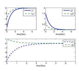
(a) The nominal system

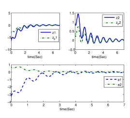
(b) The disturbed system

Figure 2: Simulations results of the descriptor system and the $\mathcal{L}_{2}-\mathcal{L}_{\infty}$ filter.

Now suppose an unknown $\mathcal{L}_{2}$ exogenous disturbance signal is affecting the system as $w(t)=30\exp(-\frac{t}{3})\cos(7t)$. Figure 2(b) shows the simulation results of $z$ and $z_{F}$ in the presence of disturbance. As expected, in the presence of disturbance, the observer filter error does not converge to zero but it is kept in the vicinity of zero such that the norm bound $\|e\|_{\infty}\leq\mu\|w\|_{2}$ is satisfied. The designed filter guarantees $\mu$ to be at most $0.1453$. The actual value of $\mu$ for this simulation is $0.0313$.

VI Conclusion

A new nonlinear $\mathcal{L}_{2}-\mathcal{L}_{\infty}$ dynamical filter design method for a class of nonlinear descriptor uncertain systems is proposed through semidefinite programming and strict LMI optimization. The proposed dynamical structure has more degree of freedom than the conventional static-gain filters and is capable of robustly stabilizing the filter error dynamics for some of those systems for which an static-gain filter can not be found. The achieved $\mathcal{L}_{2}-\mathcal{L}_{\infty}$ filter guarantees asymptotic stability of the error dynamics and is robust against time-varying parametric uncertainty.

References

• [1] Masoud Abbaszadeh and Horacio J. Marquez. Robust $H_{\infty}$ observer design for a class of nonlinear uncertain systems via convex optimization. Proceedings of the 2007 American Control Conference, New York, U.S.A., pages 1699–1704.
• [2] Masoud Abbaszadeh and Horacio J Marquez. LMI optimization approach to robust $H_{\infty}$ filtering for discrete-time nonlinear uncertain systems. In American Control Conference, 2008, pages 1905–1910, 2008.
• [3] Masoud Abbaszadeh and Horacio J. Marquez. Robust $H_{\infty}$ observer design for sampled-data Lipschitz nonlinear systems with exact and Euler approximate models. Automatica, 44(3):799–806, 2008.
• [4] Masoud Abbaszadeh and Horacio J. Marquez. LMI optimization approach to robust $H_{\infty}$ observer design and static output feedback stabilization for discrete-time nonlinear uncertain systems. International Journal of Robust and Nonlinear Control, 19(3):313–340, 2009.
• [5] Masoud Abbaszadeh and Horacio J Marquez. A generalized framework for robust nonlinear $H_{\infty}$ filtering of lipschitz descriptor systems with parametric and nonlinear uncertainties. Automatica, 48(5):894–900, 2012.
• [6] M. Boutayeb and M. Darouach. Observers design for nonlinear descriptor systems. Proceedings of the IEEE Conference on Decision and Control, 3:2369–2374, 1995.
• [7] L. Dai. Singular control systems, volume 118 of Lecture Notes on Control and Information Sciences. Springer, 1989.
• [8] M. Darouach and M. Boutayeb. Design of observers for descriptor systems. IEEE Transactions on Automatic Control, 40(7):1323–1327, 1995.
• [9] M. Darouach, M. Zasadzinski, and M. Hayar. Reduced-order observer design for descriptor systems with unknown inputs. IEEE Transactions on Automatic Control, 41(7):1068–1072, 1996.
• [10] Carlos E. de Souza, Lihua Xie, and Youyi Wang. $H_{\infty}$ filtering for a class of uncertain nonlinear systems. Systems and Control Letters, 20(6):419–426, 1993.
• [11] Huijun Gao and Changhong Wang. Robust $L_{2}-L_{\infty}$ filtering for uncertain systems with multiple time-varying state delays. Circuits and Systems I: Fundamental Theory and Applications, IEEE Transactions on, 50(4):594 – 599, april 2003.
• [12] K.M. Grigoriadis. $L_{2}$ and $L_{2}-L_{\infty}$ model reduction via linear matrix inequalities. Internation Journal of Control, 68(3):485–498, oct. 1997.
• [13] K.M. Grigoriadis and Jr. Watson, J.T. Reduced-order $H_{\infty}$ and $L_{2}-L_{\infty}$ filtering via linear matrix inequalities. Aerospace and Electronic Systems, IEEE Transactions on, 33(4):1326 –1338, oct. 1997.
• [14] Fen-Ren Chang He-Sheng Wang, Chee-Fai Yung. $H_{\infty}$ control for Nonlinear Descriptor Systems, volume 326 of Lecture Notes in Control and Information Sciences. 2006.
• [15] R. A. Horn and C. R. Johnson. Matrix Analysis. Cambrige University Press, 1985.
• [16] M. Hou and P. C. Muller. Observer design for descriptor systems. IEEE Transactions on Automatic Control, 44(1):164–169, 1999.
• [17] J. Y. Ishihara and M. H. Terra. On the Lyapunov theorem for singular systems. IEEE Transactions on Automatic Control, 47(11):1926–1930, 2002.
• [18] Pramod P. Khargonekar, Ian R. Petersen, and Kemin Zhou. Robust stabilization of uncertain linear systems: Quadratic stabilizability and $H_{\infty}$ control theory. IEEE Transactions on Automatic Control, 35(3):356–361, 1990.
• [19] J. Lofberg. YALMIP : A toolbox for modeling and optimization in MATLAB. 2004.
• [20] G. Lu and D. W. C. Ho. Full-order and reduced-order observers for Lipschitz descriptor systems: The unified LMI approach. IEEE Transactions on Circuits and Systems II: Express Briefs, 53(7), 2006.
• [21] I. Masubuchi, Y. Kamitane, A. Ohara, and N. Suda. $H_{\infty}$ control for descriptor systems: A matrix inequalities approach. Automatica, 33(4):669–673, 1997.
• [22] Xiangyu Meng and Huijun Gao. New design of robust energy-to-peak filtering for uncertain continuous-time systems. In Industrial Electronics and Applications, 2007. ICIEA 2007. 2nd IEEE Conference on, pages 1443 –1447, may 2007.
• [23] Reinaldo M. Palhares and Pedro L.D. Peres. Robust filltering with guaranteed energy-to-peak performance: an LMI approach. Automatica, 36:851–858, 2000.
• [24] Constantinos C. Pantelides. The consistent initialization of differential-algebraic systems. SIAM Journal on Scientific Computing, 9(2):219–231, 1988.
• [25] Jianbin Qiu, Gang Feng, and Jie Yang. Improved robust energy-to-peak filtering design for discrete-time switched polytopic linear systems with time-varying delay. In Intelligent Control and Automation, 2008. WCICA 2008. 7th World Congress on, pages 317 –322, june 2008.
• [26] D. N. Shields. Observer design and detection for nonlinear descriptor systems. International Journal of Control, 67(2):153–168, 1997.
• [27] Jos F. Sturm. SeDuMi. 2001.
• [28] Eiho Uezato and Masao Ikeda. Strict LMI conditions for stability, robust stabilization, and $H_{\infty}$ control of descriptor systems. Proceedings of the 38th IEEE Conference on Decision and Control, 4:4092–4097, 1999.
• [29] Youyi Wang, Lihua Xie, and Carlos E. de Souza. Robust control of a class of uncertain nonlinear systems. Systems and Control Letters, 19(2):139–149, 1992.
• [30] Ying Zhang, Ai-Guo Wu, and Guang-Ren Duan. Improved $L_{2}-L_{\infty}$ filtering for stochastic time-delay systems. International Journal of Control, Automation and Systems, 8:741–747, 2010.
• [31] Y. Zhou and J. Li. Energy-to-peak filtering for singular systems: the discrete-time case. Control Theory Applications, IET, 2(9):773 –781, sept. 2008.
• [32] G. Zimmer and J. Meier. On observing nonlinear descriptor systems. Systems and Control Letters, 32(1):43–48, 1997.