Parallel Selective Algorithms for
Nonconvex Big Data Optimization

Abstract

We propose a decomposition framework for the parallel optimization of the sum of a differentiable (possibly nonconvex) function and a (block) separable nonsmooth, convex one. The latter term is usually employed to enforce structure in the solution, typically sparsity. Our framework is very flexible and includes both fully parallel Jacobi schemes and Gauss-Seidel (i.e., sequential) ones, as well as virtually all possibilities “in between” with only a subset of variables updated at each iteration. Our theoretical convergence results improve on existing ones, and numerical results on LASSO, logistic regression, and some nonconvex quadratic problems show that the new method consistently outperforms existing algorithms.

I Introduction

The minimization of the sum of a smooth function, $F$, and of a nonsmooth (block separable) convex one, $G$,

$$\min_{\mathbf{x}\in X}V(\mathbf{x})\triangleq F(\mathbf{x})+G(\mathbf{x}),$$ (1)

is an ubiquitous problem that arises in many fields of engineering, so diverse as compressed sensing, basis pursuit denoising, sensor networks, neuroelectromagnetic imaging, machine learning, data mining, sparse logistic regression, genomics, metereology, tensor factorization and completion, geophysics, and radio astronomy. Usually the nonsmooth term is used to promote sparsity of the optimal solution, which often corresponds to a parsimonious representation of some phenomenon at hand. Many of the aforementioned applications can give rise to extremely large problems so that standard optimization techniques are hardly applicable. And indeed, recent years have witnessed a flurry of research activity aimed at developing solution methods that are simple (for example based solely on matrix/vector multiplications) but yet capable to converge to a good approximate solution in reasonable time. It is hard here to even summarize the huge amount of work done in this field; we refer the reader to the recent works [2, 3, 4, 5, 6, 7, 8, 9, 10, 11, 12, 13, 14] and books [15, 16, 17] as entry points to the literature.

However, with big data problems it is clearly necessary to design parallel methods able to exploit the computational power of multi-core processors in order to solve many interesting problems. Furthermore, even if parallel methods are used, it might be useful to reduce the number of (block) variables that are updated at each iteration, so as to alleviate the burden of dimensionality, and also because it has been observed experimentally (even if in restricted settings and under some very strong convergence assumptions, see [18, 19, 20, 13]) that this might be beneficial. While sequential solutions methods for Problem (1) have been widely investigated (especially when $F$ is convex), the analysis of parallel algorithms suitable to large-scale implementations lags behind. Gradient-type methods can of course be easily parallelized, but, in spite of their good theoretical convergence bounds. they suffer from practical drawbacks. Fist of all, they are notoriously slow in practice. Accelerated (proximal) versions have been proposed in the literature to alleviate this issue, but they require the knowledge of some function parameters (e.g., the Lipschitz constant of $\nabla F$, and the strong convexity constant of $F$, when $F$ is assumed strongly convex), which is not generally available, unless $F$ and $G$ have a very special structure (e.g., quadratic functions); (over)estimates of such parameters affect negatively the convergence speed. Moreover, all (proximal, accelerated) gradient-based schemes use only the first order information of $F$; recently we showed in [21] that exploiting the structure of $F$ by replacing its linearization with a “better” approximant can enhance practical convergence speed. However, beyond that, and looking at recent approaches, we are aware of only few (recent) papers dealing with parallel solution methods [8, 9, 10, 11, 12, 13] and [22, 23, 24, 25, 26, 20, 27]. The former group of works investigate deterministic algorithms, while the latter random ones. One advantage of the analyses in these works is that they provide a global rate of convergence. However, i) they are essentially still (regularized) gradient-based methods; ii) as proximal-gradient algorithms, they require good and global knowledge of some $F$ and $G$ parameters; and iii) except for [9, 10, 12, 26], they are proved to converge only when $F$ is convex. Indeed, to date there are no methods that are parallel and random and that can be applied to nonconvex problems. For this reason, and also because of their markedly different flavor (for example deterministic convergence vs. convergence in mean or in probability), we do not discuss further random algorithms in this paper. We refer instead to Section V for a more detailed discussion on deterministic, parallel, and sequential solution methods proposed in the literature for instances (mainly convex) of (1).

In this paper, we focus on nonconvex problems in the form (1), and proposed a new broad, deterministic algorithmic framework for the computation of their stationary solutions, which hinges on ideas first introduced in [21]. The essential, rather natural idea underlying our approach is to decompose (1) into a sequence of (simpler) subproblems whereby the function $F$ is replaced by suitable convex approximations; the subproblems can be solved in a parallel and distributed fashion and it is not necessary to update all variables at each iteration. Key features of the proposed algorithmic framework are: i) it is parallel, with a degree of parallelism that can be chosen by the user and that can go from a complete parallelism (every variable is updated in parallel to all the others) to the sequential (only one variable is updated at each iteration), covering virtually all the possibilities in “between”; ii) it permits the update in a deterministic fashion of only some (block) variables at each iteration (a feature that turns out to be very important numerically); iii) it easily leads to distributed implementations; iv) no knowledge of $F$ and $G$ parameters (e.g., the Lipschitz constant of $\nabla F$) is required; v) it can tackle a nonconvex $F$; vi) it is very flexible in the choice of the approximation of $F$, which need not be necessarily its first or second order approximation (like in proximal-gradient schemes); of course it includes, among others, updates based on gradient- or Newton-type approximations; vii) it easily allows for inexact solution of the subproblems (in some large-scale problems the cost of computing the exact solution of all the subproblems can be prohibitive); and viii) it appears to be numerically efficient. While features i)-viii), taken singularly, are certainly not new in the optimization community, we are not aware of any algorithm that possesses them all, the more so if one limits attention to methods that can handle nonconvex objective functions, which is in fact the main focus on this paper. Furthermore, numerical results show that our scheme compares favorably to existing ones.

The proposed framework encompasses a gamut of novel algorithms, offering great flexibility to control iteration complexity, communication overhead, and convergence speed, while converging under the same conditions; these desirable features make our schemes applicable to several different problems and scenarios. Among the variety of new proposed updating rules for the (block) variables, it is worth mentioning a combination of Jacobi and Gauss-Seidel updates, which seems particularly valuable in the optimization of highly nonlinear objective function; to the best of our knowledge, this is the first time that such a scheme is proposed and analyzed.

A further contribution of the paper is an extensive implementation effort over a parallel architecture (the General Computer Cluster of the Center for Computational Research at the SUNY at Buffalo), which includes our schemes and the most competitive ones in the literature. Numerical results on LASSO, Logistic Regression, and some nonconvex problems show that our algorithms consistently outperform state-of-the-art schemes.

The paper is organized as follows. Section II formally introduces the optimization problem along with the main assumptions under which it is studied. Section III describes our novel general algorithmic framework along with its convergence properties. In Section IV we discuss several instances of the general scheme introduced in Section III. Section V contains a detailed comparison of our schemes with state-of-the-art algorithms on similar problems. Numerical results are presented in Section VI. Finally, Section VII draws some conclusions. All proofs of our results are given in the Appendix.

II Problem Definition

We consider Problem (1), where the feasible set $X=X_{1}\times\cdots\times X_{N}$ is a Cartesian product of lower dimensional convex sets $X_{i}\subseteq\mathbb{R}^{n_{i}}$, and $\mathbf{x}\in\mathbb{R}^{n}$ is partitioned accordingly: $\mathbf{x}=(\mathbf{x}_{1},\ldots,\mathbf{x}_{N})$, with each $\mathbf{x}_{i}\in\mathbb{R}^{n_{i}}$; $F$ is smooth (and not necessarily convex) and $G$ is convex and possibly nondifferentiable, with $G(\mathbf{x})={\scriptstyle\sum_{i=1}^{N}}g_{i}(\mathbf{x}_{i})$. This formulation is very general and includes problems of great interest. Below we list some instances of Problem (1).

$\bullet$ $G(\mathbf{x})=0$; the problem reduces to the minimization of a smooth, possibly nonconvex problem with convex constraints.

$\bullet$ $F(\mathbf{x})=\|\mathbf{A}\mathbf{x}-\mathbf{b}\|^{2}$ and $G(\mathbf{x})=c\|\mathbf{x}\|_{1}$, $X=\mathbb{R}^{n}$, with $\mathbf{A}\in\mathbb{R}^{m\times n}$, $\mathbf{b}\in\mathbb{R}^{m}$, and $c\in\mathbb{R}_{++}$ given constants; this is the renowned and much studied LASSO problem [2].

$\bullet$ $F(\mathbf{x})=\|\mathbf{A}\mathbf{x}-\mathbf{b}\|^{2}$ and $G(\mathbf{x})=c\sum_{i=1}^{N}\|\mathbf{x}_{i}\|_{2}$, $X=\mathbb{R}^{n}$, with $\mathbf{A}\in\mathbb{R}^{m\times n}$, $\mathbf{b}\in\mathbb{R}^{m}$, and $c\in\mathbb{R}_{++}$ given constants; this is the group LASSO problem [28].

$\bullet$ $F(\mathbf{x})=\sum_{j=1}^{m}\log(1+e^{-a_{j}\mathbf{y}_{j}^{T}\mathbf{x}})$ and $G(\mathbf{x})=c\|\mathbf{x}\|_{1}$ (or $G(\mathbf{x})=c\sum_{i=1}^{N}\|\mathbf{x}_{i}\|_{2}$), with $\mathbf{y}_{i}\in\mathbb{R}^{n}$, $a_{i}\in\mathbb{R}$, and $c\in\mathbb{R}_{++}$ given constants; this is the sparse logistic regression problem [29, 30].

$\bullet$ $F(\mathbf{x})=\sum_{j=1}^{m}\max\{0,1-a_{i}\mathbf{y}_{i}^{T}\mathbf{x}\}^{2}$ and $G(\mathbf{x})=c\|\mathbf{x}\|_{1}$, with $a_{i}\in\{-1,1\}$, $\mathbf{y}_{i}\in\mathbb{R}^{n}$, and $c\in\mathbb{R}_{++}$ given; this is the $\ell_{1}$-regularized $\ell_{2}$-loss Support Vector Machine problem [5].

$\bullet$ $F(\mathbf{X}_{1},\mathbf{X}_{2})=\|\mathbf{Y}-\mathbf{X}_{1}\mathbf{X}_{2}\|_{F}^{2}$ and $G(\mathbf{X}_{2})=c\|\mathbf{X}_{2}\|_{1}$, $X=\{(\mathbf{X}_{1},\mathbf{X}_{2})\in\mathbb{R}^{n\times m}\times\mathbb{R}^{m\times N}\,:\,\|\mathbf{X}_{1}\mathbf{e}_{i}\|^{2}\leq\alpha_{i},\forall i=1,\ldots,m\}$, where $\mathbf{X}_{1}$ and $\mathbf{X}_{2}$ are the (matrix) optimization variables, $\mathbf{Y}\in\mathbb{R}^{n\times N}$, $c>0$, and $(\alpha_{i})_{i=1}^{m}>\mathbf{0}$ are given constants, $\mathbf{e}_{i}$ is the $m$-dimensional vector with a 1 in the $i$-th coordinate and $0$’s elsewhere, and $\|\mathbf{X}\|_{F}$ and $\|\mathbf{X}\|_{1}$ denote the Frobenius norm and the L1 matrix norm of $\mathbf{X}$, respectively; this is an example of the dictionary learning problem for sparse representation, see, e.g., [31]. Note that $F(\mathbf{X}_{1},\mathbf{X}_{2})$ is not jointly convex in $(\mathbf{X}_{1},\mathbf{X}_{2})$.

$\bullet$ Other problems that can be cast in the form (1) include the Nuclear Norm Minimization problem, the Robust Principal Component Analysis problem, the Sparse Inverse Covariance Selection problem, the Nonnegative Matrix (or Tensor) Factorization problem, see e.g., [32] and references therein.

Assumptions. Given (1), we make the following blanket assumptions:

(A1)

Each $X_{i}$ is nonempty, closed, and convex;

(A2)

$F$ is $C^{1}$ on an open set containing $X$;

(A3)

$\nabla F$ is Lipschitz continuous on $X$ with constant $L_{F}$;

(A4)

$G(\mathbf{x})=\sum_{i=i}^{N}g_{i}(\mathbf{x}_{i})$, with all $g_{i}$ continuous and convex on $X_{i}$;

(A5)

$V$ is coercive.

Note that the above assumptions are standard and are satisfied by most of the problems of practical interest. For instance, A3 holds automatically if $X$ is bounded; the block-separability condition A4 is a common assumption in the literature of parallel methods for the class of problems (1) (it is in fact instrumental to deal with the nonsmoothness of $G$ in a parallel environment). Interestingly A4 is satisfied by all standard $G$ usually encountered in applications, including $G(x)=\|x\|_{1}$ and $G(x)=\sum_{i=1}^{N}\|\mathbf{x}_{i}\|_{2}$, which are among the most commonly used functions. Assumption A5 is needed to guarantee that the sequence generated by our method is bounded; we could dispense with it at the price of a more complex analysis and cumbersome statement of convergence results.

III Main Results

We begin introducing an informal description of our algorithmic framework along with a list of key features that we would like our schemes enjoy; this will shed light on the core idea of the proposed decomposition technique.

We want to develop parallel solution methods for Problem (1) whereby operations can be carried out on some or (possibly) all (block) variables $\mathbf{x}_{i}$ at the same time. The most natural parallel (Jacobi-type) method one can think of is updating all blocks simultaneously: given $\mathbf{x}^{k}$, each (block) variable $\mathbf{x}_{i}$ is updated by solving the following subproblem

$$\mathbf{x}_{i}^{k+1}\in\underset{\mathbf{x}_{i}\in X_{i}}{\text{argmin}}\,\,\left\{F(\mathbf{x}_{i},\mathbf{x}_{-i}^{k})+g_{i}(\mathbf{x}_{i})\right\},$$ (2)

where $\mathbf{x}_{-i}$ denotes the vector obtained from $\mathbf{x}$ by deleting the block $\mathbf{x}_{i}$. Unfortunately this method converges only under very restrictive conditions [33] that are seldom verified in practice. To cope with this issue the proposed approach introduces some “memory" in the iterate: the new point is a convex combination of $\mathbf{x}^{k}$ and the solutions of (2). Building on this iterate, we would like our framework to enjoy many additional features, as described next.

Approximating $F$: Solving each subproblem as in (2) may be too costly or difficult in some situations. One may then prefer to approximate this problem, in some suitable sense, in order to facilitate the task of computing the new iteration. To this end, we assume that for all $i\in{\cal N}\triangleq\{1,\dots,N\}$ we can define a function $P_{i}(\mathbf{z};\mathbf{w}):X_{i}\times X\to\mathbb{R}$, the candidate approximant of $F$, having the following properties (we denote by $\nabla P_{i}$ the partial gradient of $P_{i}$ with respect to the first argument $\mathbf{z}$):

(P1)

$P_{i}(\mathbf{\bullet};\mathbf{w})$ is convex and continuously differentiable on $X_{i}$ for all $\mathbf{w}\in X$;

(P2)

$\nabla P_{i}(\mathbf{x}_{i};\mathbf{x})=\nabla_{{\mathbf{x}}_{i}}F(\mathbf{x})$ for all $\mathbf{x}\in X$;

(P3)

$\nabla P_{i}(\mathbf{z};\mathbf{\bullet})$ is Lipschitz continuous on $X$ for all $\mathbf{z}\in X_{i}$.

Such a function $P_{i}$ should be regarded as a (simple) convex approximation of $F$ at the point $\mathbf{x}$ with respect to the block of variables $\mathbf{x}_{i}$ that preserves the first order properties of $F$ with respect to $\mathbf{x}_{i}$.

Based on this approximation we can define at any point $\mathbf{x}^{k}\in X$ a regularized approximation $\widetilde{h}_{i}(\mathbf{x}_{i};\mathbf{x}^{k})$ of $V$ with respect to $\mathbf{x}_{i}$ wherein $F$ is replaced by $P_{i}$ while the nondifferentiable term is preserved, and a quadratic proximal term is added to make the overall approximation strongly convex. More formally, we have

$$\begin{array}[]{ll}&\widetilde{h}_{i}(\mathbf{x}_{i};\mathbf{x}^{k})\triangleq\underbrace{P_{i}(\mathbf{x}_{i};\mathbf{x}^{k})+\dfrac{{\tau}_{i}}{2}\left(\mathbf{x}_{i}-\mathbf{x}_{i}^{k}\right)^{T}\mathbf{Q}_{i}(\mathbf{x}^{k})\left(\mathbf{x}_{i}-\mathbf{x}^{k}_{i}\right)}_{\triangleq h_{i}(\mathbf{x}_{i};\mathbf{x}^{k})}\\ &\qquad\qquad\,\,\quad+g_{i}(\mathbf{x}_{i}),\end{array}$$ (3)

where $\mathbf{Q}_{i}(\mathbf{x}^{k})$ is an $n_{i}\times n_{i}$ positive definite matrix (possibly dependent on $\mathbf{x}^{k})$. We always assume that the functions $h_{i}(\bullet,\mathbf{x}_{i}^{k})$ are uniformly strongly convex.

(A6)

All $h_{i}(\bullet;\mathbf{x}^{k})$ are uniformly strongly convex on $X_{i}$ with a common positive definiteness constant $q>0$; furthermore, $\mathbf{Q}_{i}(\bullet)$ is Lipschitz continuous on $X$.

Note that an easy and standard way to satisfy A6 is to take, for any $i$ and for any $k$, $\tau_{i}=q>0$ and $\mathbf{Q}_{i}(\mathbf{x}^{k})=\mathbf{I}$. However, if $P_{i}(\bullet;\mathbf{x}^{k})$ is already uniformly strongly convex, one can avoid the proximal term and set $\tau_{i}=0$ while satisfying A6.

Associated with each $i$ and point $\mathbf{x}^{k}\in X$ we can define the following optimal block solution map:

$$\widehat{\mathbf{x}}_{i}(\mathbf{x}^{k},\tau_{i})\triangleq\underset{\mathbf{x}_{i}\in X_{i}}{\mbox{argmin}\,}\tilde{h}_{i}(\mathbf{x}_{i};\mathbf{x}^{k}).\vspace{-0.1cm}$$ (4)

Note that $\widehat{\mathbf{x}}_{i}(\mathbf{x}^{k},\tau_{i})$ is always well-defined, since the optimization problem in (4) is strongly convex. Given (4), we can then introduce, for each $\mathbf{y}\in X$, the solution map

$$\widehat{\mathbf{x}}(\mathbf{y},\boldsymbol{{\tau}})\triangleq\large[\widehat{\mathbf{x}}_{1}(\mathbf{y},\tau_{1}),\widehat{\mathbf{x}}_{2}(\mathbf{y},\tau_{2}),\ldots,\widehat{\mathbf{x}}_{N}(\mathbf{y},\tau_{N})\large]^{T}.$$

The proposed algorithm (that we formally describe later on) is based on the computation of (an approximation of) $\widehat{\mathbf{x}}(\mathbf{x}^{k},\boldsymbol{\tau})$. Therefore the functions $P_{i}$ should lead to as easily computable functions $\widehat{\mathbf{x}}$ as possible. An appropriate choice depends on the problem at hand and on computational requirements. We discuss alternative possible choices for the approximations $P_{i}$ in Section IV.

Inexact solutions: In many situations (especially in the case of large-scale problems), it can be useful to further reduce the computational effort needed to solve the subproblems in (4) by allowing inexact computations $\mathbf{z}^{k}$ of $\widehat{\mathbf{x}}_{i}(\mathbf{x}^{k},\tau_{i})$, i.e., $\|\mathbf{z}_{i}^{k}-\widehat{\mathbf{x}}_{i}\left(\mathbf{x}^{k},\boldsymbol{{\tau}}\right)\|\leq\varepsilon_{i}^{k}$, where $\varepsilon_{i}^{k}$ measures the accuracy in computing the solution.

Updating only some blocks: Another important feature we want for our algorithm is the capability of updating at each iteration only some of the (block) variables, a feature that has been observed to be very effective numerically. In fact, our schemes are guaranteed to converge under the update of only a subset of the variables at each iteration; the only condition is that such a subset contains at least one (block) component which is within a factor $\rho\in(0,1]$ “far away” from the optimality, in the sense explained next. Since $\mathbf{x}^{k}_{i}$ is an optimal solution of (4) if and only if $\widehat{\mathbf{x}}_{i}(\mathbf{x}^{k},\tau_{i})=\mathbf{x}^{k}_{i}$, a natural distance of $\mathbf{x}^{k}_{i}$ from the optimality is $d_{i}^{\,k}\triangleq\|\widehat{\mathbf{x}}_{i}(\mathbf{x}^{k},\tau_{i})-\mathbf{x}^{k}_{i}\|$; one could then select the blocks $\mathbf{x}_{i}$’s to update based on such an optimality measure (e.g., opting for blocks exhibiting larger $d_{i}^{\,k}$’s). However, this choice requires the computation of all the solutions $\widehat{\mathbf{x}}_{i}(\mathbf{x}^{k},\tau_{i})$, for $i=1,\ldots,n$, which in some applications (e.g., huge-scale problems) might be computationally too expensive. Building on the same idea, we can introduce alternative less expensive metrics by replacing the distance $\|\widehat{\mathbf{x}}_{i}(\mathbf{x}^{k},\tau_{i})-\mathbf{x}^{k}_{i}\|$ with a computationally cheaper error bound, i.e., a function $E_{i}(\mathbf{x})$ such that

$$\underline{s}_{i}\|\widehat{\mathbf{x}}_{i}(\mathbf{x}^{k},\tau_{i})-\mathbf{x}^{k}_{i}\|\leq E_{i}(\mathbf{x}^{k})\leq\bar{s}_{i}\|\widehat{\mathbf{x}}_{i}(\mathbf{x}^{k},\tau_{i})-\mathbf{x}^{k}_{i}\|,\vspace{-0.1cm}$$ (5)

for some $0<\underline{s}_{i}\leq\bar{s}_{i}$. Of course one can always set $E_{i}(\mathbf{x}^{k})=\|\widehat{\mathbf{x}}_{i}(\mathbf{x}^{k},\tau_{i})-\mathbf{x}^{k}_{i}\|$, but other choices are also possible; we discuss this point further in Section IV.

Algorithmic framework: We are now ready to formally introduce our algorithm, Algorithm 1, that includes all the features discussed above; convergence to stationary solutions of (1) is stated in Theorem 1.

 Algorithm 1: Inexact Flexible Parallel Algorithm (FLEXA)

 $\textbf{Data}:$ $\{\varepsilon_{i}^{k}\}$ for $i\in\mathcal{N}$, $\boldsymbol{{\tau}}\geq\mathbf{0}$, $\{\gamma^{k}\}>0$, $\mathbf{x}^{0}\in X$, $\rho\in(0,1]$.

Set $k=0$.

$\mbox{(S.1)}:$  If $\mathbf{x}^{k}$ satisfies a termination criterion: STOP;

$\mbox{(S.2)}:$ Set $M^{k}\triangleq\max_{i}\{E_{i}(\mathbf{x}^{k})\}$.

Choose a set $S^{k}$ that contains at least one index $i$

for which $E_{i}(\mathbf{x}^{k})\geq\rho M^{k}.$

$\mbox{(S.3)}:$ For all $i\in S^{k}$, solve (4) with accuracy $\varepsilon_{i}^{k}:$

Find $\mathbf{z}_{i}^{k}\in X_{i}$ s.t. $\|\mathbf{z}_{i}^{k}-\widehat{\mathbf{x}}_{i}\left(\mathbf{x}^{k},\boldsymbol{{\tau}}\right)\|\leq\varepsilon_{i}^{k}$;

Set $\widehat{\mathbf{z}}^{k}_{i}=\mathbf{\mathbf{z}}_{i}^{k}$ for $i\in S^{k}$ and $\widehat{\mathbf{z}}^{k}_{i}=\mathbf{x}^{k}_{i}$ for $i\not\in S^{k}$

$\mbox{(S.4)}:$ Set $\mathbf{x}^{k+1}\triangleq\mathbf{x}^{k}+\gamma^{k}\,(\widehat{\mathbf{z}}^{k}-\mathbf{x}^{k})$;

$\mbox{(S.5)}:$ $k\leftarrow k+1$, and go to $\mbox{(S.1)}.$

 

Theorem 1.

Let $\{\mathbf{x}^{k}\}$ be the sequence generated by Algorithm III, under A1-A6. Suppose that $\{\gamma^{k}\}$ and $\{\varepsilon_{i}^{k}\}$ satisfy the following conditions: i) $\gamma^{k}\in(0,1]$; ii) $\sum_{k}\gamma^{k}=+\infty$; iii) $\sum_{k}\left(\gamma^{k}\right)^{2}<+\infty$; and iv) $\varepsilon_{i}^{k}\leq\gamma^{k}\alpha_{1}\min\{\alpha_{2},1/\|\nabla_{\mathbf{x}_{i}}F(\mathbf{x}^{k})\|\}$ for all $i\in{\cal N}$ and some $\alpha_{1}>0$ and $\alpha_{2}>0$. Additionally, if inexact solutions are used in Step 3, i.e., $\varepsilon_{i}^{k}>0$ for some $i$ and infinite $k$, then assume also that $G$ is globally Lipschitz on $X$. Then, either Algorithm III converges in a finite number of iterations to a stationary solution of (1) or every limit point of $\{\mathbf{x}^{k}\}$ (at least one such points exists) is a stationary solution of (1).

Proof.

See Appendix A-B.∎

The proposed algorithm is extremely flexible. We can always choose $S^{k}={\cal N}$ resulting in the simultaneous update of all the (block) variables (full Jacobi scheme); or, at the other extreme, one can update a single (block) variable per time, thus obtaining a Gauss-Southwell kind of method. More classical cyclic Gauss-Seidel methods can also be derived and are discussed in the next subsection. One can also compute inexact solutions (Step 3) while preserving convergence, provided that the error term $\varepsilon_{i}^{k}$ and the step-size $\gamma^{k}$’s are chosen according to Theorem 1; some practical choices for these parameters are discussed in Section IV. We emphasize that the Lipschitzianity of $G$ is required only if $\widehat{\mathbf{x}}(\mathbf{x}^{k},\tau)$ is not computed exactly for infinite iterations. At any rate this Lipschitz conditions is automatically satisfied if $G$ is a norm (and therefore in LASSO and group LASSO problems for example) or if $X$ is bounded.

As a final remark, note that versions of Algorithm III where all (or most of) the variables are updated at each iteration are particularly amenable to implementation in distributed environments (e.g., multi-user communications systems, ad-hoc networks, etc.). In fact, in this case, not only the calculation of the inexact solutions $z^{k}_{i}$ can be carried out in parallel, but the information that “the $i$-th subproblem” has to exchange with the “other subproblem” in order to compute the next iteration is very limited. A full appreciation of the potentialities of our approach in distributed settings depends however on the specific application under consideration and is beyond the scope of this paper. We refer the reader to [21] for some examples, even if in less general settings.

III-A Gauss-Jacobi algorithms

Algorithm III and its convergence theory cover fully parallel Jacobi as well as Gauss-Southwell-type methods, and many of their variants. In this section we show that Algorithm 1 can also incorporate hybrid parallel-sequential (Jacobi$-$Gauss-Seidel) schemes wherein block of variables are updated simultaneously by sequentially computing entries per block. This procedure seems particularly well suited to parallel optimization on multi-core/processor architectures.

Suppose that we have $P$ processors that can be used in parallel and we want to exploit them to solve Problem (1) ($P$ will denote both the number of processors and the set $\{1,2,\ldots,P\}$). We “assign” to each processor $p$ the variables $I_{p}$; therefore $I_{1},\ldots,I_{P}$ is a partition of $I$. We denote by $\mathbf{x}_{p}\triangleq(\mathbf{x}_{pi})_{i\in I_{p}}$ the vector of (block) variables $\mathbf{x}_{pi}$ assigned to processor $p$, with $i\in I_{p}$; and $\mathbf{x}_{-p}$ is the vector of remaining variables, i.e., the vector of those assigned to all processors except the $p$-th one. Finally, given $i\in I_{p}$, we partition $\mathbf{x}_{p}$ as $\mathbf{x}_{p}=(\mathbf{x}_{pi<},\mathbf{x}_{pi\geq})$, where $\mathbf{x}_{pi<}$ is the vector containing all variables in $I_{p}$ that come before $i$ (in the order assumed in $I_{p}$), while $\mathbf{x}_{pi\geq}$ are the remaining variables. Thus we will write, with a slight abuse of notation $\mathbf{x}=(\mathbf{x}_{pi<},\mathbf{x}_{pi\geq},\mathbf{x}_{-p})$.

Once the optimization variables have been assigned to the processors, one could in principle apply the inexact Jacobi Algorithm III. In this scheme each processor $p$ would compute sequentially, at each iteration $k$ and for every (block) variable $\mathbf{x}_{pi}$, a suitable $\mathbf{z}^{k}_{pi}$ by keeping all variables but $\mathbf{x}_{pi}$ fixed to $(\mathbf{x}^{k}_{pj})_{i\neq j\in I_{p}}$ and $\mathbf{x}^{k}_{-p}$. But since we are solving the problems for each group of variables assigned to a processor sequentially, this seems a waste of resources; it is instead much more efficient to use, within each processor, a Gauss-Seidel scheme, whereby the current calculated iterates are used in all subsequent calculations. Our Gauss-Jacobi method formally described in Algorithm 2 implements exactly this idea; its convergence properties are given in Theorem 2.

 Algorithm 2: Inexact Gauss-Jacobi Algorithm

 $\textbf{Data}:$ $\{\varepsilon_{pi}^{k}\}$ for $p\in P$ and $i\in{I}_{p}$, $\boldsymbol{{\tau}}\geq\mathbf{0}$, $\{\gamma^{k}\}>0$, $\mathbf{x}^{0}\in\mathcal{K}$.

Set $k=0$.

$\mbox{(S.1)}:$  If $\mathbf{x}^{k}$ satisfies a termination criterion: STOP;

$\mbox{(S.2)}:$ For all $p\in P$ do (in parallel),

For all $i\in I_{p}$ do (sequentially)

a) Find $\mathbf{z}^{k}_{pi}\in\mathcal{X}_{i}$ s.t.

$\|\mathbf{z}_{pi}^{k}-\widehat{{\mathbf{x}}}_{pi}\left((\mathbf{x}_{pi<}^{k+1},\mathbf{x}_{pi\geq}^{k},\mathbf{x}_{-p}^{k}),\boldsymbol{{\tau}}\right)\|\leq\varepsilon_{pi}^{k}$;

b) Set ${\mathbf{x}}_{pi}^{k+1}\triangleq{\mathbf{x}}_{pi}^{k}+{\gamma}^{\,k}\,\left(\mathbf{z}_{pi}^{k}-{\mathbf{x}}_{pi}^{k}\right)$

$\mbox{(S.3)}:$ $k\leftarrow k+1$, and go to $\mbox{(S.1)}.$

 

Theorem 2.

Let $\{\mathbf{x}^{k}\}_{k=1}^{\infty}$ be the sequence generated by Algorithm III-A, under the setting of Theorem 1, but with the addition assumption that $\nabla F$ is bounded on $\mathcal{X}$. Then, either Algorithm III-A converges in a finite number of iterations to a stationary solution of (1) or every limit point of the sequence $\{\mathbf{x}^{k}\}_{k=1}^{\infty}$ (at least one such points exists) is a stationary solution of (1).

Proof.

See Appendix A-C. ∎

Although the proof of Theorem 2 is relegated to the appendix, it is interesting to point out that the gist of the proof is to show that Algorithm III-A is nothing else but an instance of Algorithm III with errors. We remark that Algorithm III-A contains as special case the classical cyclical Gauss-Seidel scheme it is sufficient to set $P=1$ then a single processor updates all the (scalar) variables sequentially while using the new values of those that have already been updated.
By updating all variables at each iteration, Algorithm III-A has the advantage that neither the error bounds $E_{i}$ nor the exact solutions $\widehat{\mathbf{x}}_{pi}$ need to be computed, in order to decide which variables should be updated. Furthermore it is rather intuitive that the use of the “latest available information” should reduce the number of overall iterations needed to converge with respect to Algorithm III. However this advantages should be weighted against the following two facts: i) updating all variables at each iteration might not always be the best (or a feasible) choice; and ii) in many practical instances of Problem (1), using the latest information as dictated by Algorithm III-A may require extra calculations, e.g. to compute function gradients, and communication overhead (these aspects are discussed on specific examples in Section VI). It may then be of interest to consider a further scheme, that we might call “Gauss-Jacobi with Selection”, where we merge the basic ideas of Algorithms III and III-A. Roughly speaking, at each iteration we proceed as in the Gauss-Jacobi Algorithm III-A, but we perform the Gauss steps only on a subset ${S}^{k}_{p}$ of each $I_{p}$, where the subset ${S}^{k}_{p}$ is defined according to the rules used in Algorithm III. To present this combined scheme, we need to extend the notation used in Algorithm III-A. Let ${S}^{k}_{p}$ be a subset of $I_{p}$. For notational purposes only, we reorder $\mathbf{x}_{p}$ so that first we have all variables in ${S}^{k}_{p}$ and then the remaining variables in $I_{p}$: $\mathbf{x}_{p}=(\mathbf{x}_{{S}^{k}_{p}},\mathbf{x}_{I_{p}\setminus{S}^{k}_{p}})$. Now, similarly to what done before, and given an index $i\in{S}^{k}_{p}$, we partition $\mathbf{x}_{{S}^{k}_{p}}$ as $\mathbf{x}_{{S}^{k}_{p}}=(\mathbf{x}_{{S}^{k}_{p}i<},\mathbf{x}_{{S}^{k}_{p}i\geq})$, where $\mathbf{x}_{{S}^{k}_{p}i<}$ is the vector containing all variables in ${S}^{k}_{p}$ that come before $i$ (in the order assumed in ${S}^{k}_{p}$), while $\mathbf{x}_{{S}^{k}_{p}i\geq}$ are the remaining variables in ${S}^{k}_{p}$. Thus we will write, with a slight abuse of notation $\mathbf{x}=(\mathbf{x}_{{S}^{k}_{p}i<},\mathbf{x}_{{S}^{k}_{p}i\geq},\mathbf{x}_{-p})$. The proposed Gauss-Jacobi with Selection is formally described in Algorithm 3 below.

 Algorithm 3: Inexact GJ Algorithm with Selection

 $\textbf{Data}:$ $\{\varepsilon_{pi}^{k}\}$ for $p\in P$ and $i\in{I}_{p}$, $\boldsymbol{{\tau}}\geq\mathbf{0}$, $\{\gamma^{k}\}>0$, $\mathbf{x}^{0}\in\mathcal{K}$,

$\rho\in(0,1]$. Set $k=0$.

$\mbox{(S.1)}:$  If $\mathbf{x}^{k}$ satisfies a termination criterion: STOP;

$\mbox{(S.2)}:$ Set $M^{k}\triangleq\max_{i}\{E_{i}(\mathbf{x}^{k})\}$.

Choose sets $S^{k}_{p}\subseteq I_{p}$ so that their union $S^{k}$ contains

at least one index $i$ for which $E_{i}(\mathbf{x}^{k})\geq\rho M^{k}.$

$\mbox{(S.3)}:$ For all $p\in P$ do (in parallel),

For all $i\in S^{k}_{p}$ do (sequentially)

a) Find $\mathbf{z}^{k}_{pi}\in\mathcal{X}_{i}$ s.t.

$\|\mathbf{z}_{pi}^{k}-\widehat{{\mathbf{x}}}_{pi}\left((\mathbf{x}_{{S}^{k}_{p}i<}^{k+1},\mathbf{x}_{{S}^{k}_{p}i\geq}^{k},\mathbf{x}_{-p}^{k}),\boldsymbol{{\tau}}\right)\|\leq\varepsilon_{pi}^{k}$;

b) Set ${\mathbf{x}}_{pi}^{k+1}\triangleq{\mathbf{x}}_{pi}^{k}+{\gamma}^{\,k}\,\left(\mathbf{z}_{pi}^{k}-{\mathbf{x}}_{pi}^{k}\right)$

$\mbox{(S.4)}:$ Set $\mathbf{x}^{k+1}_{pi}=\mathbf{x}^{k}_{pi}$ for all $i\not\in S^{k}$,

$k\leftarrow k+1$, and go to $\mbox{(S.1)}.$

 

Theorem 3.

Let $\{\mathbf{x}^{k}\}_{k=1}^{\infty}$ be the sequence generated by Algorithm III-A, under the setting of Theorem 1, but with the addition assumption that $\nabla F$ is bounded on $\mathcal{X}$. Then, either Algorithm III-A converges in a finite number of iterations to a stationary solution of (1) or every limit point of the sequence $\{\mathbf{x}^{k}\}_{k=1}^{\infty}$ (at least one such points exists) is a stationary solution of (1).

Proof.

The proof is just a (notationally complicated, but conceptually easy) combination of the proofs of Theorems 1 and 2 and is omitted for lack of space. ∎

Our experiments show that, in the case of highly nonlinear objective functions, Algorithm 3 performs very well in practice, see Section VI.

IV Examples and Special cases

Algorithms III and III-A are very general and encompass a gamut of novel algorithms, each corresponding to various forms of the approximant $P_{i}$, the error bound function $E_{i}$, the step-size sequence $\gamma^{k}$, the block partition, etc. These choices lead to algorithms that can be very different from each other, but all converging under the same conditions. These degrees of freedom offer a lot of flexibility to control iteration complexity, communication overhead, and convergence speed. We outline next several effective choices for the design parameters along with some illustrative examples of specific algorithms resulting from a proper combination of these choices.

On the choice of the step-size $\gamma^{k}$. An example of step-size rule satisfying conditions i)-iv) in Theorem 1 is: given $0<\gamma^{0}\leq 1$, let

$$\gamma^{k}=\gamma^{k-1}\left(1-\theta\,\gamma^{k-1}\right),\quad k=1,\ldots,$$ (6)

where $\theta\in(0,1)$ is a given constant. Notice that while this rule may still require some tuning for optimal behavior, it is quite reliable, since in general we are not using a (sub)gradient direction, so that many of the well-known practical drawbacks associated with a (sub)gradient method with diminishing step-size are mitigated in our setting. Furthermore, this choice of step-size does not require any form of centralized coordination, which is a favorable feature in a parallel environment. Numerical results in Section VI show the effectiveness of (the customization of) (6) on specific problems.

Remark 4 (Line-search variants of Algorithms III and III-A).

It is possible to prove convergence of Algorithms 1 and III-A also using other step-size rules, for example Armijo-like line-search procedures on $V$. In fact, Proposition 8 in Appendix A shows that the direction $\widehat{\mathbf{x}}\left(\mathbf{x}^{k},\boldsymbol{{\tau}}\right)-\mathbf{x}^{k}$ is a “good" descent direction. Based on this result, it is not difficult to prove that if $\gamma^{k}$ is chosen by a suitable line-search procedure on $V$, convergence of Algorithm 1 to stationary points of Problem (1) (in the sense of Theorem 1) is guaranteed. Note that standard line-search methods proposed for smooth functions cannot be applied to $V$ (due to the nonsmooth part $G$); one needs to rely on more sophisticated procedures, e.g., in the spirit of those proposed in [10, 6, 37, 12]. We provide next an example of line-search rule that can be used to compute $\gamma^{k}$ while guaranteeing convergence of Algorithms 1 and 2 [instead of using rules i)-iii) in Theorem 1]; because of space limitations, we consider only the case of exact solutions (i.e., $\epsilon_{i}^{k}=0$ in Algorithm 1 and $\epsilon_{pi}^{k}=0$ in Algorithms 2 and 3). Writing for short $\widehat{\mathbf{x}}_{i}^{k}\triangleq\widehat{\mathbf{x}}_{i}\left(\mathbf{x}^{k},\boldsymbol{{\tau}}\right)$ and $\Delta\widehat{\mathbf{x}}^{k}\triangleq(\Delta\widehat{\mathbf{x}}^{k}_{i})_{i=1}^{n}$, with $\Delta\widehat{\mathbf{x}}^{k}_{i}\triangleq\widehat{\mathbf{x}}_{i}^{k}-\mathbf{x}_{i}^{k}$, and denoting by $(\mathbf{x})_{\mathcal{S}^{k}}$ the vector whose component $i$ is equal to $x_{i}$ if $i\in\mathcal{S}^{k}$, and zero otherwise, we have the following: let $\alpha,\beta\in(0,1)$, choose $\gamma^{k}=\beta^{\bar{\ell}}$, where $\bar{\ell}$ is the smallest nonnegative integer $\ell$ such that

$$V\left(\mathbf{x}^{k}+\beta^{\ell}(\Delta\widehat{\mathbf{x}}^{k})_{\mathcal{S}^{k}}\right)-V(\mathbf{x}^{k})\leq-\alpha\cdot\beta^{\ell}\,\|\left(\Delta\widehat{\mathbf{x}}^{k}\right)_{\mathcal{S}^{k}}\|^{2}.$$

Of course, the above procedure will likely be more efficient in terms of iterations than the one based on diminishing step-size rules [as (6)]. However, performing a line-search on a multicore architecture requires some shared memory and coordination among the cores/processors; therefore we do not consider further this variant. Finally, we observe that convergence of Algorithms 1 and 2 can also be obtained by choosing a constant (suitably small ) stepsize $\gamma^{k}$. This is actually the easiest option, but since it generally leads to extremely slow convergence we omitted this option from our developments here.

On the choice of the error bound function $E_{i}(\mathbf{x})$.
$\bullet$ As we mentioned, the most obvious choice is to take $E_{i}(\mathbf{x})=\|\widehat{\mathbf{x}}_{i}(\mathbf{x}^{k},\tau_{i})-\mathbf{x}^{k}_{i}\|$. This is a valuable choice if the computation of $\widehat{\mathbf{x}}_{i}(\mathbf{x}^{k},\tau_{i})$ can be easily accomplished. For instance, in the LASSO problem with ${\cal N}=\{1,\ldots,n\}$ (i.e., when each block reduces to a scalar variable), it is well-known that $\widehat{\mathbf{x}}_{i}(\mathbf{x}^{k},\tau_{i})$ can be computed in closed form using the soft-thresholding operator [11].
$\bullet$ In situations where the computation of $\|\widehat{\mathbf{x}}_{i}(\mathbf{x}^{k},\tau_{i})-\mathbf{x}^{k}_{i}\|$ is not possible or advisable, we can resort to estimates. Assume momentarily that $G\equiv 0$. Then it is known [34, Proposition 6.3.1] under our assumptions that $\|\Pi_{X_{i}}(\mathbf{x}^{k}_{i}-\nabla_{\mathbf{x}_{i}}F(\mathbf{x}^{k}))-\mathbf{x}^{k}_{i}\|$ is an error bound for the minimization problem in (4) and therefore satisfies (5), where $\Pi_{X_{i}}(\mathbf{y})$ denotes the Euclidean projection of $\mathbf{y}$ onto the closed and convex set $X_{i}$. In this situation we can choose $E_{i}(\mathbf{x}^{k})=\|\Pi_{X_{i}}(\mathbf{x}^{k}_{i}-\nabla_{\mathbf{x}_{i}}F(\mathbf{x}^{k}))-\mathbf{x}^{k}_{i}\|$. If $G(\mathbf{x})\not\equiv 0$ things become more complex. In most cases of practical interest, adequate error bounds can be derived from [10, Lemma 7].
$\bullet$ It is interesting to note that the computation of $E_{i}$ is only needed if a partial update of the (block) variables is performed. However, an option that is always feasible is to take $S^{k}={\cal N}$ at each iteration, i.e., update all (block) variables at each iteration. With this choice we can dispense with the computation of $E_{i}$ altogether.
On the choice of the approximant $P_{i}(\mathbf{x}_{i};\mathbf{x})$.
$\bullet$ The most obvious choice for $P_{i}$ is the linearization of $F$ at $\mathbf{x}^{k}$ with respect to $\mathbf{x}_{i}$:

$$P_{i}(\mathbf{x}_{i};\mathbf{x}^{k})=F(\mathbf{x}^{k})+\nabla_{\mathbf{x}_{i}}F(\mathbf{x}^{k})^{T}(\mathbf{x}_{i}-\mathbf{x}_{i}^{k}).$$

With this choice, and taking for simplicity $\mathbf{Q}_{i}(\mathbf{x}^{k})=\mathbf{I}$,

$$\begin{array}[]{ll}\widehat{\mathbf{x}}_{i}(\mathbf{x}^{k},\tau_{i})=\underset{\mathbf{x}_{i}\in X_{i}}{\mbox{argmin}\,}\left\{F(\mathbf{x}^{k})+\nabla_{\mathbf{x}_{i}}F(\mathbf{x}^{k})^{T}(\mathbf{x}_{i}-\mathbf{x}_{i}^{k})\right.\\ \left.\hskip 91.04872pt+\dfrac{\tau_{i}}{2}\|\mathbf{x}_{i}-\mathbf{x}_{i}^{k}\|^{2}+g_{i}(\mathbf{x}_{i})\right\}.\vspace{-0.1cm}\end{array}$$ (7)

This is essentially the way a new iteration is computed in most (block-)CDMs for the solution of (group) LASSO problems and its generalizations.
$\bullet$ At another extreme we could just take $P_{i}(\mathbf{x}_{i};\mathbf{x}^{k})=F(\mathbf{x}_{i},\mathbf{x}_{-i}^{k})$. Of course, to have P1 satisfied (cf. Section III), we must assume that $F(\mathbf{x}_{i},\mathbf{x}_{-i}^{k})$ is convex. With this choice, and setting for simplicity $\mathbf{Q}_{i}(\mathbf{x}^{k})=\mathbf{I}$, we have

$$\widehat{\mathbf{x}}_{i}(\mathbf{x}^{k},\tau_{i})\triangleq\underset{\mathbf{x}_{i}\in X_{i}}{\mbox{argmin}\,}\left\{F(\mathbf{x}_{i},\mathbf{x}^{k}_{-i})+\frac{\tau_{i}}{2}\|\mathbf{x}_{i}-\mathbf{x}_{i}^{k}\|^{2}+g_{i}(\mathbf{x}_{i})\right\},$$ (8)

thus giving rise to a parallel nonlinear Jacobi type method for the constrained minimization of $V(\mathbf{x})$.
$\bullet$ Between the two “extreme” solutions proposed above, one can consider “intermediate” choices. For example, If $F(\mathbf{x}_{i},\mathbf{x}_{-i}^{k})$ is convex, we can take $P_{i}(\mathbf{x}_{i};\mathbf{x}^{k})$ as a second order approximation of $F(\mathbf{x}_{i},\mathbf{x}_{-i}^{k})$, i.e.,

$$\begin{array}[]{ll}P_{i}(\mathbf{x}_{i};\mathbf{x}^{k})=F(\mathbf{x}^{k})+\nabla_{\mathbf{x}_{i}}F(\mathbf{x}^{k})^{T}(\mathbf{x}_{i}-\mathbf{x}_{i}^{k})\vskip 3.0pt plus 1.0pt minus 1.0pt\\ \hskip 56.9055pt+\frac{1}{2}(\mathbf{x}_{i}-\mathbf{x}_{i}^{k})^{T}\nabla^{2}_{\mathbf{x}_{i}\mathbf{x}_{i}}F(\mathbf{x}^{k})(\mathbf{x}_{i}-\mathbf{x}_{i}^{k}).\end{array}$$ (9)

When $g_{i}(\mathbf{x}_{i})\equiv 0$, this essentially corresponds to taking a Newton step in minimizing the “reduced” problem $\min_{\mathbf{x}_{i}\in X_{i}}F(\mathbf{x}_{i},\mathbf{x}_{-i}^{k})$, resulting in

$$\begin{array}[]{lll}\widehat{\mathbf{x}}_{i}(\mathbf{x}^{k},\tau_{i})&=\underset{\mathbf{x}_{i}\in X_{i}}{\mbox{argmin}\,}\left\{F(\mathbf{x}^{k})+\nabla_{\mathbf{x}_{i}}F(\mathbf{x}^{k})^{T}(\mathbf{x}_{i}-\mathbf{x}_{i}^{k})\right.\vspace{-0.1cm}\\ &\;\hskip 42.67912pt+\left.\frac{1}{2}(\mathbf{x}_{i}-\mathbf{x}_{i}^{k})^{T}\nabla^{2}_{\mathbf{x}_{i}\mathbf{x}_{i}}F(\mathbf{x}^{k})(\mathbf{x}_{i}-\mathbf{x}_{i}^{k})\right.\vskip 6.0pt plus 2.0pt minus 2.0pt\\ &\;\hskip 42.67912pt\left.+\frac{\tau_{i}}{2}\|\mathbf{x}_{i}-\mathbf{x}_{i}^{k}\|^{2}+g_{i}(\mathbf{x}_{i})\right\}.\end{array}$$ (10)

$\bullet$ Another “intermediate” choice, relying on a specific structure of the objective function that has important applications is the following. Suppose that $F$ is a sum-utility function, i.e.,

$$F(\mathbf{x})=\sum_{j\in J}f_{j}(\mathbf{x}_{i},\mathbf{x}_{-i}),$$

for some finite set $J$. Assume now that for every $j\in S_{i}\subseteq J$, the functions $f_{j}(\bullet,\mathbf{x}_{-i})$ is convex. Then we may set

$$P_{i}(\mathbf{x}_{i};\mathbf{x}^{k})=\sum_{j\in S_{i}}f_{j}(\mathbf{x}_{i},\mathbf{x}_{-i}^{k})+\sum_{j\not\in S_{i}}\nabla f_{j}(\mathbf{x}_{i},\mathbf{x}_{-i}^{k})^{T}(\mathbf{x}_{i}-\mathbf{x}_{i}^{k})$$

thus preserving, for each $i$, the favorable convex part of $F$ with respect to $\mathbf{x}_{i}$ while linearizing the nonconvex parts. This is the approach adopted in [21] in the design of multi-users systems, to which we refer for applications in signal processing and communications.

The framework described in Algorithm III can give rise to very different schemes, according to the choices one makes for the many variable features it contains, some of which have been detailed above. Because of space limitation, we cannot discuss here all possibilities. We provide next just a few instances of possible algorithms that fall in our framework.

Example$\,\#$1$-$(Proximal) Jacobi algorithms for convex functions. Consider the simplest problem falling in our setting: the unconstrained minimization of a continuously differentiable convex function, i.e., assume that $F$ is convex, $G\equiv 0$, and $X=\mathbb{R}^{n}$. Although this is possibly the best studied problem in nonlinear optimization, classical parallel methods for this problem [33, Sec. 3.2.4] require very strong contraction conditions. In our framework we can take $P_{i}(\mathbf{x}_{i};\mathbf{x}^{k})=F(\mathbf{x}_{i},\mathbf{x}_{-i}^{k})$, resulting in a parallel Jacobi-type method which does not need any additional assumptions. Furthermore our theory shows that we can even dispense with the convexity assumption and still get convergence of a Jacobi-type method to a stationary point. If in addition we take $S^{k}={\cal N}$, we obtain the class of methods studied in [35, 36, 37, 21].

Example$\,\#$2$-$Parallel coordinate descent methods for LASSO. Consider the LASSO problem, i.e., Problem (1) with $F(\mathbf{x})=\|\mathbf{A}\mathbf{x}-\mathbf{b}\|^{2}$, $G(\mathbf{x})=c\|\mathbf{x}\|_{1}$, and $X=\mathbb{R}^{n}$. Probably, to date, the most successful class of methods for this problem is that of CDMs, whereby at each iteration a single variable is updated using (7). We can easily obtain a parallel version for this method by taking $n_{i}=1$, $S^{k}={\cal N}$ and still using (7). Alternatively, instead of linearizing $F$, we can better exploit the structure of $F$ and use (8). In fact, it is well known that in LASSO problems subproblem (8) can be solved analytically (when $n_{i}=1$). We can easily consider similar methods for the group LASSO problem as well (just take $n_{i}>1$).

Example$\,\#$3$-$Parallel coordinate descent methods for Logistic Regression. Consider the Logistic Regression problem, i.e., Problem (1) with $F(\mathbf{x})=\sum_{j=1}^{m}\log(1+e^{-a_{i}\mathbf{y}_{i}^{T}\mathbf{x}})$, $G(\mathbf{x})=c\|\mathbf{x}\|_{1}$, and $X=\mathbb{R}^{n}$, where $\mathbf{y}_{i}\in\mathbb{R}^{n}$, $a_{i}\in\{-1,1\}$, and $c\in\mathbb{R}_{++}$ are given constants. Since $F(\mathbf{x}_{i},\mathbf{x}_{-i}^{k})$ is convex, we can take $P_{i}(\mathbf{x}_{i};\mathbf{x}^{k})=F(\mathbf{x}^{k})+\nabla_{\mathbf{x}_{i}}F(\mathbf{x}^{k})^{T}$ $(\mathbf{x}_{i}-\mathbf{x}_{i}^{k})+\frac{1}{2}(\mathbf{x}_{i}-\mathbf{x}_{i}^{k})^{T}\nabla^{2}_{\mathbf{x}_{i}\mathbf{x}_{i}}F(\mathbf{x}^{k})(\mathbf{x}_{i}-\mathbf{x}_{i}^{k})$ and thus obtaining a fully distributed and parallel CDM that uses a second order approximation of the smooth function $F$. Moreover by taking $n_{i}=1$ and using a soft-thresholding operator, each $\widehat{\mathbf{x}}_{i}$ can be computed in closed form.

Example$\,\#$4$-$Parallel algorithms for dictionary learning problems. Consider the dictionary learning problem, i.e., Problem (1) with $F(\mathbf{X})=\|\mathbf{Y}-\mathbf{X}_{1}\mathbf{X}_{2}\|_{F}^{2}$ and $G(\mathbf{X}_{2})=c\|\mathbf{X}_{2}\|_{1}$, and $X=\{\mathbf{X}\triangleq(\mathbf{X}_{1},\mathbf{X}_{2})\in\mathbb{R}^{n\times m}\times\mathbb{R}^{m\times N}\,:\,\|\mathbf{X}_{1}\mathbf{e}_{i}\|^{2}\leq\alpha_{i},\forall i=1,\ldots,m\}$. Since $F(\mathbf{X}_{1},\mathbf{X}_{2})$ is convex in $\mathbf{X}_{1}$ and $\mathbf{X}_{2}$ separately, one can take $P_{1}(\mathbf{X}_{1};\mathbf{X}_{2}^{k})=F(\mathbf{X}_{1},\mathbf{X}_{2}^{k})$ and $P_{2}(\mathbf{X}_{2};\mathbf{X}_{1}^{k})=F(\mathbf{X}_{1}^{k},\mathbf{X}_{2})$. Although natural, this choice does not lead to a close form solutions of the subproblems associated with the optimization of $\mathbf{X}_{1}$ and $\mathbf{X}_{2}$. This desirable property can be obtained using the following alternative approximations of $F$ [38]: $P_{1}(\mathbf{X}_{1};\mathbf{X}^{k})=F(\mathbf{X}^{k})+\left\langle\nabla_{\mathbf{X_{1}}}F(\mathbf{X}^{k}),\mathbf{X}_{1}-\mathbf{X}_{1}^{k}\right\rangle$ and $P_{2}(\mathbf{X}_{2};\mathbf{X}^{k})=F(\mathbf{X}^{k})+\left\langle\nabla_{\mathbf{X_{2}}}F(\mathbf{X}^{k}),\mathbf{X}_{2}-\mathbf{X}_{2}^{k}\right\rangle$, where $\left\langle\mathbf{A},\mathbf{B}\right\rangle\triangleq\text{tr}(\mathbf{A}^{T}\mathbf{B})$. Note that differently from [38], our algorithm is parallel and more flexible in the choice of the proximal gain terms [cf. (3)].

V Related works

The proposed algorithmic framework draws on Successive Convex Approximation (SCA) paradigms that have a long history in the optimization literature. Nevertheless, our algorithms and their convergence conditions (cf. Theorems 1 and 2) unify and extend current parallel and sequential SCA methods in several directions, as outlined next.

(Partially) Parallel Methods: The roots of parallel deterministic SCA schemes (wherein all the variables are updated simultaneously) can be traced back at least to the work of Cohen on the so-called auxiliary principle [35, 36] and its related developments, see e.g. [8, 9, 10, 11, 12, 23, 13, 27, 21, 37, 39, 40]. Roughly speaking these works can be divided in two groups, namely: solution methods for convex objective functions [8, 11, 23, 13, 27, 35, 36] and nonconvex ones [9, 10, 12, 21, 37, 39, 40]. All methods in the former group (and [9, 10, 12, 39, 40]) are (proximal) gradient schemes; they thus share the classical drawbacks of gradient-like schemes (cf. Sec. I); moreover, by replacing the convex function $F$ with its first order approximation, they do not take any advantage of any structure of $F$ beyond mere differentiability; exploiting any available structural properties of $F$, instead, has been shown to enhance (practical) convergence speed, see e.g. [21]. Comparing with the second group of works [9, 10, 12, 21, 37, 39, 40], our algorithmic framework improves on their convergence properties while adding great flexibility in the selection of how many variables to update at each iteration. For instance, with the exception of [10, 18, 19, 20, 13], all the aforementioned works do not allow parallel updates of only a subset of all variables, a feature that instead, fully explored as we do, can dramatically improve the convergence speed of the algorithm, as we show in Section VI. Moreover, with the exception of [37], they all require an Armijo-type line-search, which makes them not appealing for a (parallel) distributed implementation. A scheme in [37] is actually based on diminishing step-size-rules, but its convergence properties are quite weak: not all the limit points of the sequence generated by this scheme are guaranteed to be stationary solutions of (1).

Our framework instead i) deals with nonconvex (nonsmooth) problems; ii) allows one to use a much varied array of approximations for $F$ and also inexact solutions of the subproblems; iii) is fully parallel and distributed (it does not rely on any line-search); and iv) leads to the first distributed convergent schemes based on very general (possibly) partial updating rules of the optimization variables. In fact, among deterministic schemes, we are aware of only three algorithms [10, 23, 13] performing at each iteration a parallel update of only a subset of all the variables. These algorithms however are gradient-like schemes, and do not allow inexact solutions of the subproblems, when a closed form solution is not available (in some large-scale problems the cost of computing the exact solution of all the subproblems can be prohibitive). In addition, [10] requires an Armijo-type line-search whereas [23] and [13] are applicable only to convex objective functions and are not fully parallel. In fact, convergence conditions therein impose a constraint on the maximum number of variables that can be simultaneously updated, a constraint that in many large scale problems is likely not satisfied.

Sequential Methods: Our framework contains as special cases also sequential updates; it is then interesting to compare our results to sequential schemes too. Given the vast literature on the subject, we consider here only the most recent and general work [14]. In [14] the authors consider the minimization of a possibly nonsmooth function by Gauss-Seidel methods whereby, at each iteration, a single block of variables is updated by minimizing a global upper convex approximation of the function. However, finding such an approximation is generally not an easy task, if not impossible. To cope with this issue, the authors also proposed a variant of their scheme that does not need this requirement but uses an Armijo-type line-search, which however makes the scheme not suitable for a parallel/distributed implementation. Contrary to [14], in our framework conditions on the approximation function (cf. P1-P3) are trivial to be satisfied (in particular, $P$ need not be an upper bound of $F$), enlarging significantly the class of utility functions $V$ which the proposed solution method is applicable to. Furthermore, our framework gives rise to parallel and distributed methods (no line search is used) whose degree of parallelism can be chosen by the user.

VI Numerical Results

In this section we provide some numerical results showing solid evidence of the viability of our approach. Our aim is to compare to state-of-the-art methods as well as test the influence of two key features of the proposed algorithmic framework, namely: parallelism and selective (greedy) selection of (only some) variables to update at each iteration. The tests were carried out on i) LASSO and Logistic Regression problems, two of the most studied (convex) instances of Problem (1); and ii) nonconvex quadratic programming.

All codes have been written in C++. All algebra is performed by using the Intel Math Kernel Library (MKL). The algorithms were tested on the General Compute Cluster of the Center for Computational Research at the SUNY Buffalo. In particular we used a partition composed of 372 DELL 16x2.20GHz Intel E5-2660 “Sandy Bridge” Xeon Processor computer nodes with 128 Gb of DDR4 main memory and QDR InfiniBand 40Gb/s network card. In our experiments, parallel algorithms have been tested using up to 40 parallel processes (8 nodes with 5 cores per each), while sequential algorithms ran on a single process (using thus one single core).

VI-A LASSO problem

We implemented the instance of Algorithm 1 described in Example # 2 in the previous section, using the approximating function $P_{i}$ as in (8). Note that in the case of LASSO problems $\widehat{x}_{i}(\mathbf{x}^{k},\tau_{i})$, the unique solution (8), can be easily computed in closed form using the soft-thresholding operator, see [11].

Tuning of Algorithm 1: In the description of our algorithmic framework we considered fixed values of $\tau_{i}$, but it is clear that varying them a finite number of times does not affect in any way the theoretical convergence properties of the algorithms. We found that the following choices work well in practice: (i) $\tau_{i}$ are initially all set to $\displaystyle\tau_{i}=\text{tr}(\mathbf{A}^{T}\mathbf{A})/2n$, i.e., to half of the mean of the eigenvalues of $\nabla^{2}F$; (ii) all $\tau_{i}$ are doubled if at a certain iteration the objective function does not decrease; and (iii) they are all halved if the objective function decreases for ten consecutive iterations or the relative error on the objective function $\texttt{re}(\mathbf{x})$ is sufficiently small, specifically if

$$\texttt{re}(\mathbf{x})\triangleq\frac{V(\mathbf{x})-V^{*}}{V^{*}}\leq 10^{-2},$$ (11)

where $V^{*}$ is the optimal value of the objective function $V$ (in our experiments on LASSO $V^{*}$ is known). In order to avoid increments in the objective function, whenever all $\tau_{i}$ are doubled, the associated iteration is discarded, and in (S.4) of Algorithm 1 it is set $\mathbf{x}^{k+1}=\mathbf{x}^{k}$. In any case we limited the number of possible updates of the values of $\tau_{i}$ to 100.

The step-size $\gamma^{k}$ is updated according to the following rule:

$$\gamma^{k}=\gamma^{k-1}\left(1-\min\left\{1,\frac{10^{-4}}{\texttt{re}(\mathbf{x}^{k})}\right\}\theta\,\gamma^{k-1}\right),\quad k=1,\ldots,\vspace{-0.1cm}$$ (12)

with $\gamma^{0}=0.9$ and $\theta=1e-7$. The above diminishing rule is based on (6) while guaranteeing that $\gamma^{k}$ does not become too close to zero before the relative error is sufficiently small.

Finally the error bound function is chosen as $E_{i}(\mathbf{x}^{k})=\|\widehat{\mathbf{x}}_{i}(\mathbf{x}^{k},\tau_{i})-\mathbf{x}_{i}^{k}\|$, and $S^{k}$ in Step 2 of the algorithm is set to

$$S^{k}=\{i:E_{i}(\mathbf{x}^{k})\geq\sigma M^{k}\}.$$

In our tests we consider two options for $\sigma$, namely: i) $\sigma=0$, which leads to a fully parallel scheme wherein at each iteration all variables are updated; and ii) $\sigma=0.5$, which corresponds to updating only a subset of all the variables at each iteration. Note that for both choices of $\sigma$, the resulting set $S^{k}$ satisfies the requirement in (S.2) of Algorithm III; indeed, $S^{k}$ always contains the index $i$ corresponding to the largest $E_{i}(\mathbf{x}^{k})$. We term the above instance of Algorithm 1 FLEXible parallel Algorithm (FLEXA), and we will refer to these two versions as FLEXA $\sigma=0$ and FLEXA $\sigma=0.5$. Note that both versions satisfy conditions of Theorem 1, and thus are convergent.

Algorithms in the literature: We compared our versions of FLEXA with the most competitive distributed and sequential algorithms proposed in the literature to solve the LASSO problem. More specifically, we consider the following schemes.

$\bullet$ FISTA: The Fast Iterative Shrinkage-Thresholding Algorithm (FISTA) proposed in [11] is a first order method and can be regarded as the benchmark algorithm for LASSO problems. Building on the separability of the terms in the objective function $V$, this method can be easily parallelized and thus take advantage of a parallel architecture. We implemented the parallel version that use a backtracking procedure to estimate the Lipschitz constant $L_{F}$ of $\nabla F$ [11].

$\bullet$ SpaRSA: This is the first order method proposed in [12]; it is a popular spectral projected gradient method that uses a spectral step length together with a nonmonotone line search to enhance convergence. Also this method can be easily parallelized, which is the version implemented in our tests. In all the experiments we set the parameters of SpaRSA as in [12]: $M=5$, $\sigma=0.01$, $\alpha_{\max}=1e30$, and $\alpha_{\min}=1e-30$.

$\bullet$ GRock $\&$ Greedy-1BCD: GRock is a parallel algorithm proposed in [13] that performs well on sparse LASSO problems. We tested the instance of GRock where the number of variables simultaneously updated is equal to the number of the parallel processors. It is important to remark that the theoretical convergence properties of GRock are in jeopardy as the number of variables updated in parallel increases; roughly speaking, GRock is guaranteed to converge if the columns of the data matrix $\mathbf{A}$ in the LASSO problem are “almost” orthogonal, a feature that is not satisfied in many applications. A special instance with convergence guaranteed is the one where only one block per time (chosen in a greedy fashion) is updated; we refer to this special case as greedy-1BCD.

$\bullet$ ADMM: This is a classical Alternating Method of Multipliers (ADMM). We implemented the parallel version as proposed in [41].

In the implementation of the parallel algorithms, the data matrix $\mathbf{A}$ of the LASSO problem is generated in a uniform column block distributed manner. More specifically, each processor generates a slice of the matrix itself such that the overall one can be reconstructed as $\mathbf{A}=\left[\mathbf{A}_{1}\,\mathbf{A}_{2}\,\cdots\,\mathbf{A}_{P}\right]$, where $P$ is the number of parallel processors, and $\mathbf{A}_{i}$ has $n/P$ columns for each $i$. Thus the computation of each product $\mathbf{A}\mathbf{x}$ (which is required to evaluate $\nabla F$) and the norm $\|\mathbf{x}\|_{1}$ (that is $G$) is divided into the parallel jobs of computing $\mathbf{A}_{i}\mathbf{x}_{i}$ and $\|\mathbf{x}_{i}\|_{1}$, followed by a reducing operation.
Numerical Tests: We generated six groups of LASSO problems using the random generator proposed by Nesterov [9], which permits to control the sparsity of the solution. For the first five groups, we considered problems with 10,000 variables and matrix $\mathbf{A}$ having 9,000 rows. The five groups differ in the degree of sparsity of the solution; more specifically the percentage of non zeros in the solution is 1%, 10%, 20%, 30%, and 40%, respectively. The last group is formed by instances with 100,000 variables and 5000 rows for $\mathbf{A}$, and solutions having 1% of non zero variables. In all experiments and for all the algorithms, the initial point was set to the zero vector.

Results of our experiments for the 10,000 variables groups are reported in Fig. 1, where we plot the relative error as defined in (11) versus the CPU time; all the curves are obtained using 40 cores, and averaged over ten independent random realizations. Note that the CPU time includes communication times (for distributed algorithms) and the initial time needed by the methods to perform all pre-iteration computations (this explains why the curves of ADMM start after the others; in fact ADMM requires some nontrivial initializations). For one instance, the one corresponding to 1% of the sparsity of the solution, we plot also the relative error versus iterations [Fig. 2(a2)]; similar behaviors of the algorithms have been observed also for the other instances, and thus are not reported. Results for the LASSO instance with 100,000 variables are plotted in Fig. 2. The curves are averaged over five random realizations.

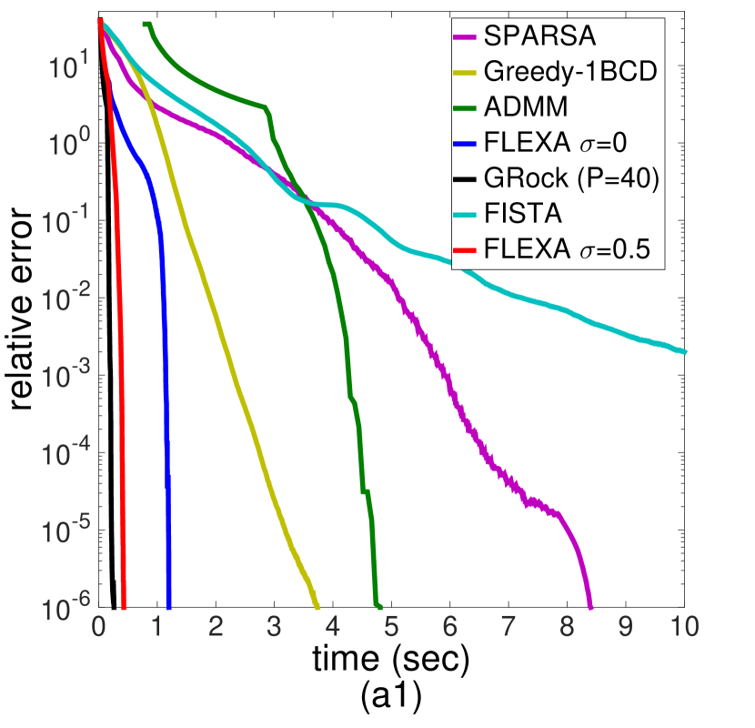
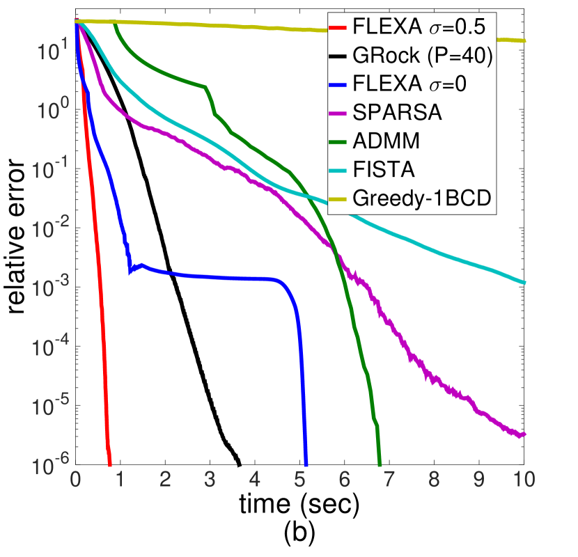
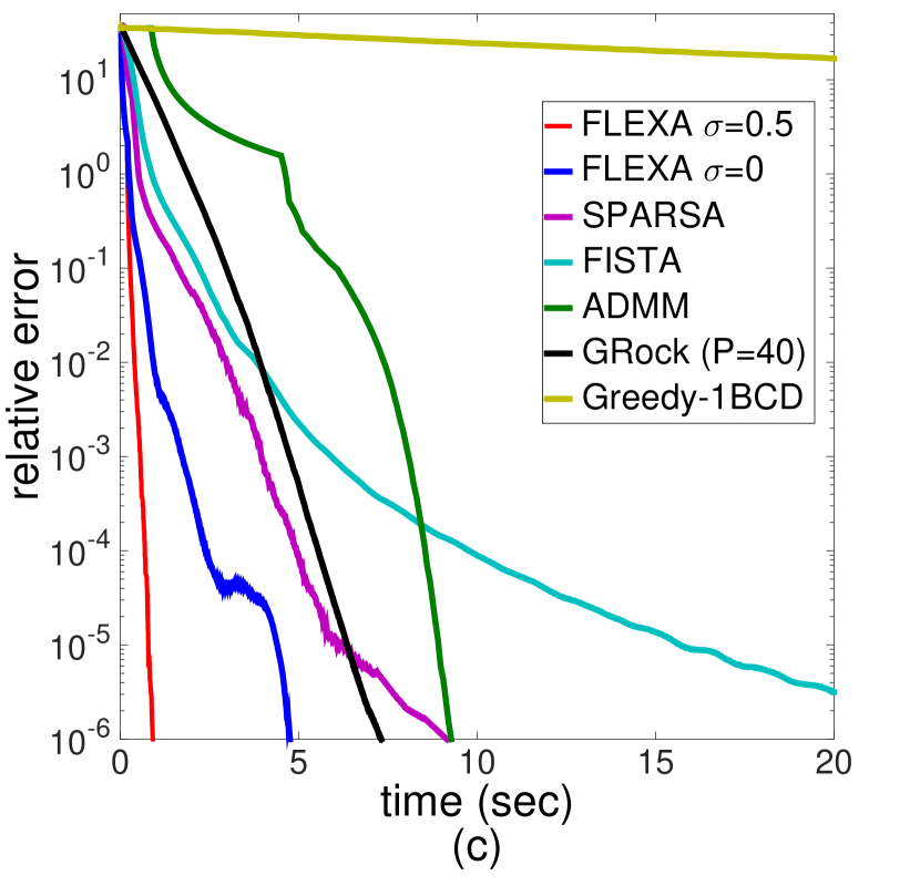
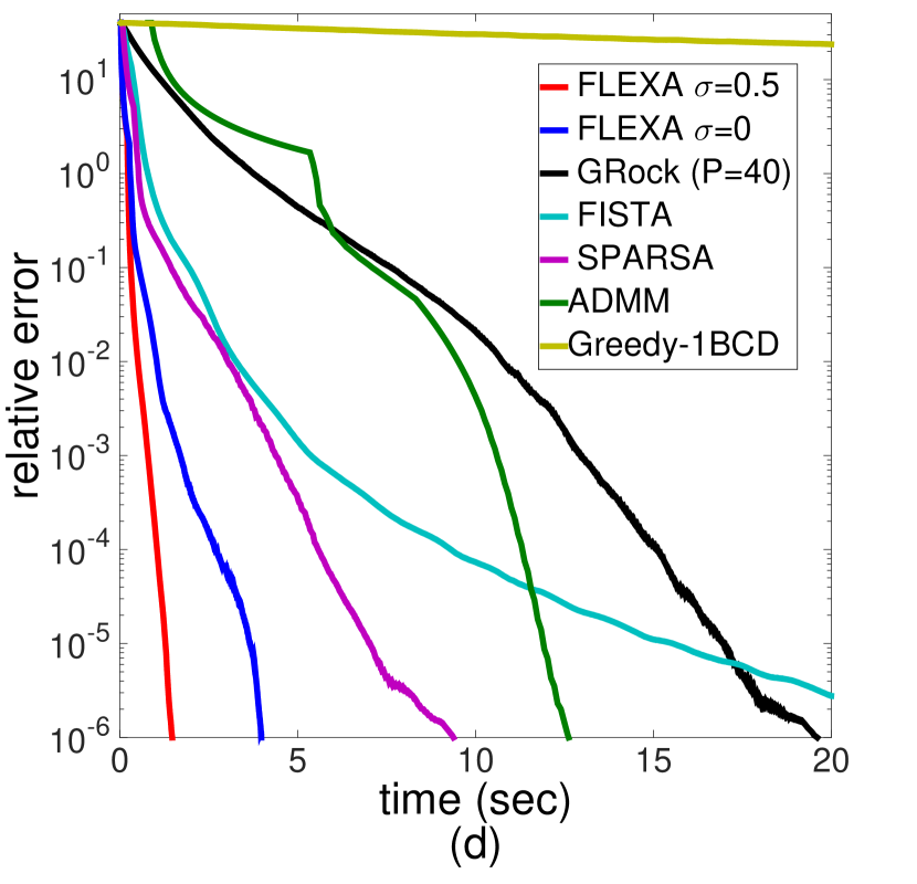
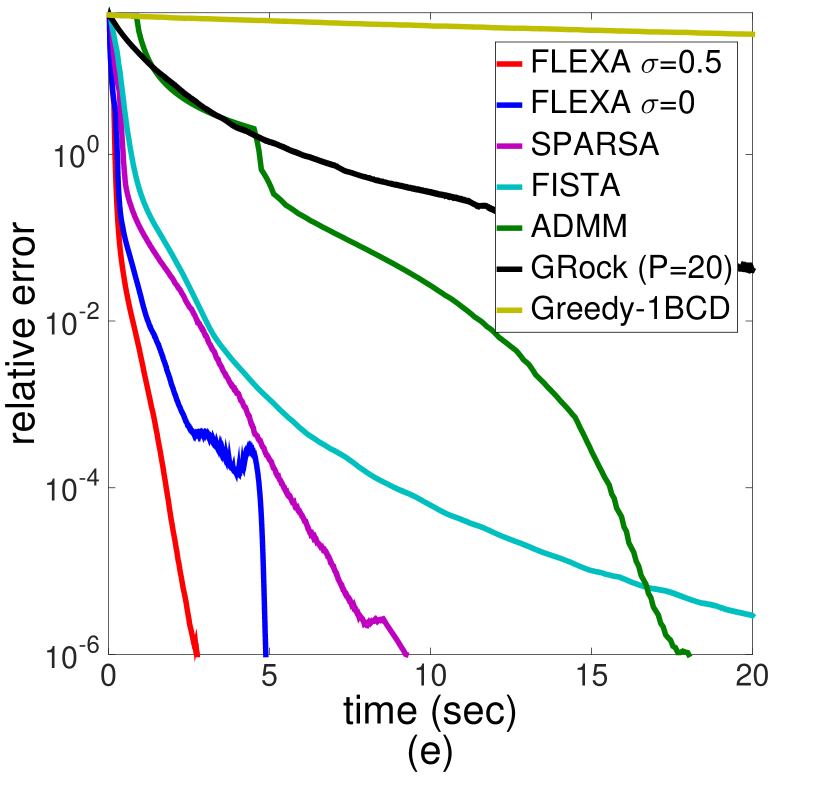
Figure 1: LASSO with 10,000 variables; relative error vs. time (in seconds) for: (a1) 1% non zeros - (b) 10% non zeros - (c) 20% non zeros - (d) 30% non zeros - (e) 40% non zeros; (a2) relative error vs. iterations for 1% non zeros.

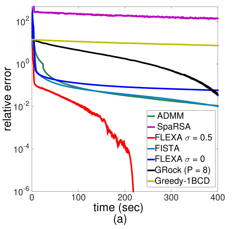
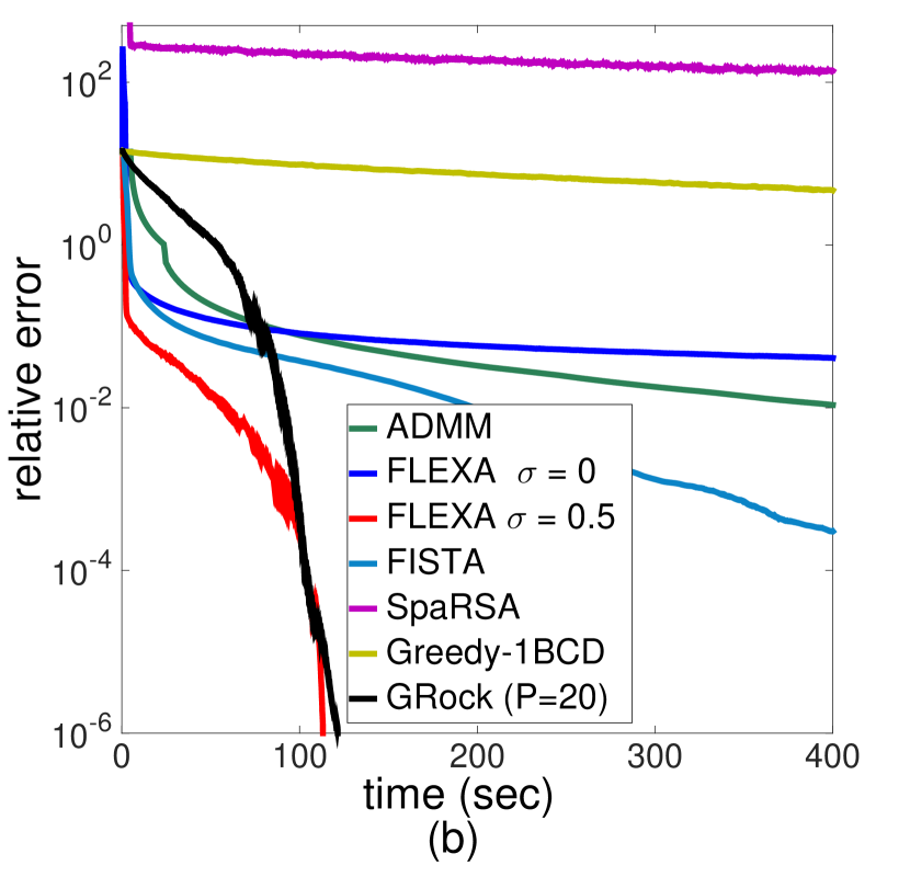
Figure 2: LASSO with $10^{5}$ variables; Relative error vs. time for: (a) 8 cores - (b) 20 cores.

Given Fig. 1 and 2, the following comments are in order. On all the tested problems, FLEXA $\sigma=0.5$ outperforms in a consistent manner all other implemented algorithms. In particular, as the sparsity of the solution decreases, the problems become harder and the selective update operated by FLEXA ($\sigma=0.5$) improves over FLEXA ($\sigma=0$), where instead all variables are updated at each iteration. FISTA is capable to approach relatively fast low accuracy when the solution is not too sparse, but has difficulties in reaching high accuracy. SpaRSA seems to be very insensitive to the degree of sparsity of the solution; it behaves well on 10,000 variables problems and not too sparse solutions, but is much less effective on very large-scale problems. The version of GRock with $P=40$ is the closest match to FLEXA, but only when the problems are very sparse (but it is not supported by a convergence theory on our test problems). This is consistent with the fact that its convergence properties are at stake when the problems are quite dense. Furthermore, if the problem is very large, updating only 40 variables at each iteration, as GRock does, could slow down the convergence, especially when the optimal solution is not very sparse. From this point of view, FLEXA $\sigma=0.5$ seems to strike a good balance between not updating variables that are probably zero at the optimum and nevertheless update a sizeable amount of variables when needed in order to enhance convergence.

Remark 5 (On parallelism).

Fig. 2 shows that FLEXA seems to exploit well parallelism on LASSO problems. Indeed, when passing from 8 to 20 cores, the running time approximately halves. This kind of behavior has been consistently observed also for smaller problems and different number of cores; because of the space limitation, we do not report these experiments. Note that practical speed-up due to the use of a parallel architecture is given by several factor that are not easily predictable and very dependent on the specific problem at hand, including communication times among the cores, the data format, etc. In this paper we do not pursue a theoretical study of the speed-up that, given the generality of our framework, seems a challenging goal. We finally observe that GRock appears to improve greatly with the number of cores. This is due to the fact that in GRock the maximum number of variables that is updated in parallel is exactly equal to the number of cores (i.e., the degree of parallelism), and this might become a serious drawback on very large problems (on top of the fact that convergence is in jeopardy). On the contrary, our theory permits the parallel update of any number of variables while guaranteeing convergence.

Remark 6 (On selective updates).

It is interesting to comment why FLEXA $\sigma=0.5$ behaves better than FLEXA $\sigma=0$. To understand the reason behind this apparently counterintuitive phenomenon, we first note that Algorithm III has the remarkable capability to identify those variables that will be zero at a solution; because of lack of space, we do not provide here the proof of this statement but only an informal description. Roughly speaking, it can be shown that, for $k$ large enough, those variables that are zero in $\widehat{\mathbf{x}}(\mathbf{x}^{k},\boldsymbol{\tau})$ will be zero also in a limiting solution $\bar{\mathbf{x}}$. Therefore, suppose that $k$ is large enough so that this identification property already takes place (we will say that “we are in the identification phase”) and consider an index $i$ such that $\bar{x}_{i}=0$. Then, if $x^{k}_{i}$ is zero, it is clear, by Steps 3 and 4, that $x^{k^{\prime}}_{i}$ will be zero for all indices $k^{\prime}>k$, independently of whether $i$ belongs to $S^{k}$ or not. In other words, if a variable that is zero at the solution is already zero when the algorithm enters the identification phase, that variable will be zero in all subsequent iterations; this fact, intuitively, should enhance the convergence speed of the algorithm. Conversely, if when we enter the identification phase $x^{k}_{i}$ is not zero, the algorithm will have to bring it back to zero iteratively. It should then be clear why updating only variables that we have “strong” reason to believe will be non zero at a solution is a better strategy than updating them all. Of course, there may be a problem dependence and the best value of $\sigma$ can vary from problem to problem. But we believe that the explanation outlined above gives firm theoretical ground to the idea that it might be wise to “waste" some calculations and perform only a partial update of the variables. $\square$

VI-B Logistic regression problems

The logistic regression problem is described in Example #3 (cf. Section III) and is a highly nonlinear problem involving many exponentials that, notoriously, give rise to numerical difficulties. Because of these high nonlinearities, a Gauss-Seidel approach is expected to be more effective than a pure Jacobi method, a fact that was confirmed by our preliminary tests. For this reason, for the logistic regression problem we tested also an instance of Algorithm III-A; we term it GJ-FLEXA. The setting of the free parameters in GJ-FLEXA is essentially the same described for LASSO, but with the following differences:

(a)

The approximant $P_{i}$ is chosen as the second order approximation of the original function $F$ (Ex. #3, Sec. III);

(b)

The initial $\tau_{i}$ are set to $\text{tr}(\mathbf{Y}^{T}\mathbf{Y})/2n$ for all $i$, where $n$ is the total number of variables and $\mathbf{Y}=[\mathbf{y}_{1}\,\mathbf{y}_{2}\,\cdots\,\mathbf{y}_{m}]^{\scriptscriptstyle T}.$

(c)

Since the optimal value $V^{*}$ is not known for the logistic regression problem, we no longer use $\texttt{re}(\mathbf{x})$ as merit function but $\|\mathbf{Z}(\mathbf{x})\|_{\infty}$, with $\mathbf{Z}(\mathbf{x})=\nabla F(\mathbf{x})-\Pi_{[-c,c]^{n}}\left(\nabla F(\mathbf{x})-\mathbf{x}\right).$ Here the projection $\Pi_{[-c,c]^{n}}(\mathbf{z})$ can be efficiently computed; it acts component-wise on $\mathbf{z}$, since $[-c,c]^{n}=[-c,c]\times\cdots\times[-c,c]$. Note that $Z(\mathbf{x})$ is a valid optimality measure function; indeed, $\mathbf{Z}(\mathbf{x})=\mathbf{0}$ is equivalent to the standard necessary optimality condition for Problem (1), see [6]. Therefore, whenever $\texttt{re}(\mathbf{x})$ was used for the Lasso problems, we now use $\|\mathbf{Z}(\mathbf{x})\|_{\infty}$ [including in the step- size rule (12)].

We tested the algorithms on three instances of the logistic regression problem that are widely used in the literature, and whose essential data features are given in Table I; we downloaded the data from the LIBSVM repository http://www.csie.ntu.edu.tw/$\sim$cjlin/libsvm/, which we refer to for a detailed description of the test problems. In our implementation, the matrix $\mathbf{Y}$ is stored in a column block distributed manner $\mathbf{Y}=\left[\mathbf{Y}_{1}\,\mathbf{Y}_{2}\,\cdots\,\mathbf{Y}_{P}\right]$, where $P$ is the number of parallel processors. We compared FLEXA ($\sigma=0.5)$ and GJ-FLEXA with the other parallel algorithms (whose tuning of the free parameters is the same as in Fig. 1 and Fig. 2), namely: FISTA, SpaRSA, and GRock. For the logistic regression problem, we also tested one more algorithm, that we call CDM. This Coordinate Descent Method is an extremely efficient Gauss-Seidel-type method (customized for logistic regression), and is part of the LIBLINEAR package available at http://www.csie.ntu.edu.tw/$\sim$cjlin/.

In Fig. 3, we plotted the relative error vs. the CPU time (the latter defined as in Fig. 1 and Fig. 2) achieved by the aforementioned algorithms for the three datasets, and using a different number of cores, namely: 8, 16, 20, 40; for each algorithm but GJ-FLEXA we report only the best performance over the aforementioned numbers of cores. Note that in order to plot the relative error, we had to preliminary estimate $V^{*}$ (which is not known for logistic regression problems). To do so, we ran GJ-FLEXA until the merit function value $\|Z(\mathbf{x}^{k})\|_{\infty}$ went below $10^{-7}$, and used the corresponding value of the objective function as estimate of $V^{*}$. We remark that we used this value only to plot the curves. Next to each plot, we also reported the overall FLOPS counted up till reaching the relative errors as indicated in the table. Note that the FLOPS of GRock on real-sim and rcv1 are those counted in 24 hours simulation time; when terminated, the algorithm achieved a relative error that was still very far from the reference values set in our experiment. Specifically, GRock reached $1.16$ (instead of $1e-4$) on real-sim and $0.58$ (instead of $1e-3$) on rcv1; the counted FLOPS up till those error values are still reported in the tables.

Data set	$m$	$n$	$c$
gisette (scaled)	$6000$	$5000$	$0.25$
real-sim	$72309$	$20958$	$4$
rcv1	$677399$	$47236$	$4$

TABLE I: Data sets for logistic regression tests

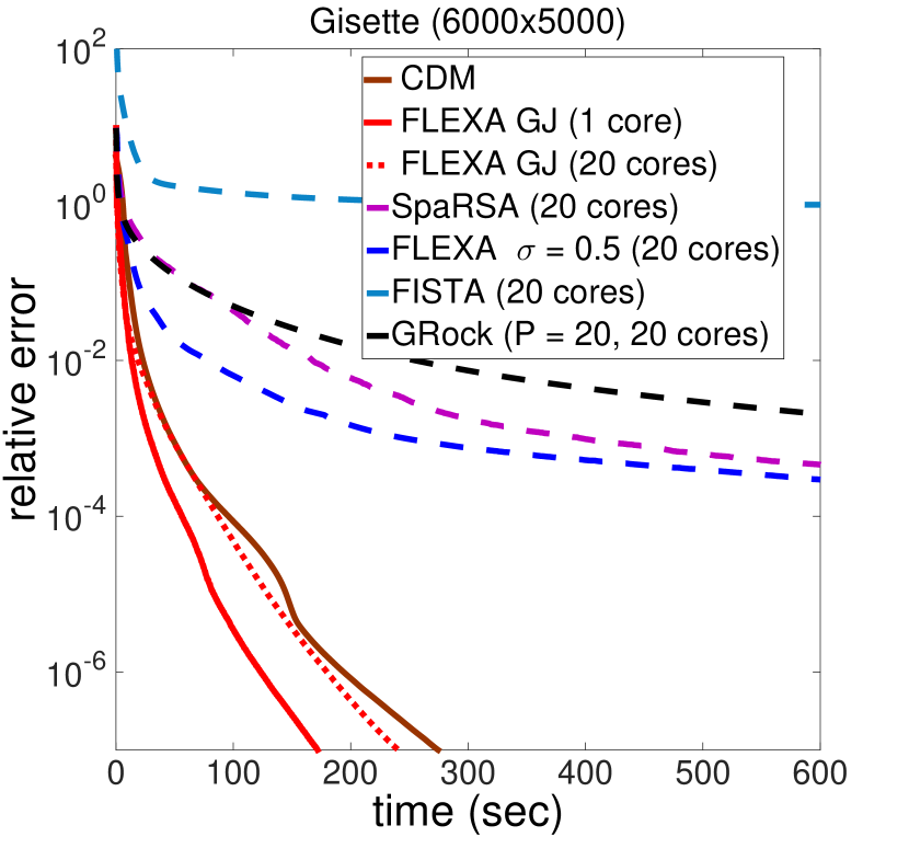
Algo.	FLOPS (1e-2/1e-6)
GJ-FLEXA (1C)	1.30e+10/1.23e+11
GJ-FLEXA (20C)	5.18e+11/5.07e+12
FLEXA $\!\sigma\!=\!0.5$ (20C)	1.88e+12/4.06e+13
CDM	2.15e+10/1.68e+11
SpaRSA (20C)	2.20e+12/5.37e+13
FISTA (20C)	3.99e+12/5.66e+13
GroCK (20C)	7.18e+12/1.81e+14

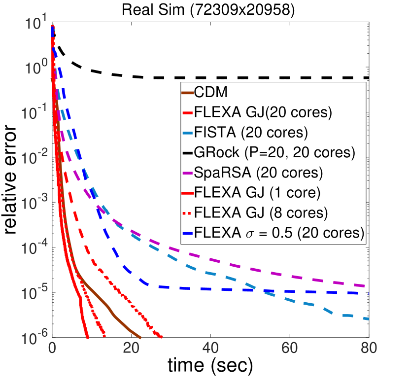
Algorithms	FLOPS (1e-4/1e-6)
GJ-FLEXA (1C)	2.76e+9/6.60e+9
GJ-FLEXA (20C)	9.83e+10/2.85e+11
FLEXA $\!\sigma\!=\!0.5$ (20C)	3.54e+10/4.69e+11
CDM	4.43e+9/2.18e+10
SpaRSA (20C)	7.18e+9/1.94e+11
FISTA (20C)	3.91e+10/1.56e+11
GroCK (20C)	8.30e+14 (after 24h)

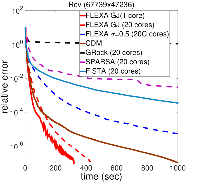
Algorithms	FLOPS (1e-3/1e-6)
GJ-FLEXA (1C)	3.61e+10/2.43e+11
GJ-FLEXA (20C)	1.35e+12/6.22e+12
FLEXA $\!\sigma\!=\!0.5$ (20C)	8.53e+11/7.19e+12
CDM	5.60e+10/6.00e+11
SpaRSA (20C)	9.38e+12/7.20e+13
FISTA (20C)	2.58e+12/2.76e+13
GroCK (20C)	1.72e+15 (after 24h)

Figure 3: Logistic Regression problems: Relative error vs. time (in seconds) and FLOPS for i) gisette, ii) real-sim, and iii) rcv.

The analysis of the figures shows that, due to the high nonlinearities of the objective function, the more performing methods are the Gauss-Seidel-type ones. In spite of this, FLEXA still behaves quite well. But GJ-FLEXA with one core, thus a non parallel method, clearly outperforms all other algorithms. The explanation can be the following. GJ-FLEXA with one core is essentially a Gauss-Seidel-type method but with two key differences: the use of a stepsize and more importantly a (greedy) selection rule by which only some variables are updated at each round. As the number of cores increases, the algorithm gets “closer and closer” to a Jacobi-type method, and because of the high nonlinearities, moving along a “Jacobi direction” does not bring improvements. In conclusion, for logistic regression problems, our experiments suggests that while the (opportunistic) selection of variables to update seems useful and brings to improvements even in comparison to the extremely efficient, dedicated CDM algorithm/software, parallelism (at least, in the form embedded in our scheme), does not appear to be beneficial as instead observed for LASSO problems.

VI-C Nonconvex quadratic problems

We consider now a nonconvex instance of Problem (1); because of space limitation, we present some preliminary results only on non convex quadratic problems; a more detailed analysis of the behavior of our method in the nonconvex case is an important topic that is the subject of a forthcoming paper. Nevertheless, current results suggest that FLEXA’s good behavior on convex problems extends to the nonconvex setting.

Consider the following nonconvex instance of Problem (1):

$${\displaystyle\begin{array}[]{cl}{\displaystyle{\min_{\mathbf{x}}}}&\underset{F(\mathbf{x})}{\underbrace{\|\mathbf{A}\mathbf{x}-\mathbf{b}\|^{2}-\bar{c}\|\mathbf{x}\|^{2}}}+\underset{G(\mathbf{x})}{\underbrace{c\|\mathbf{x}\|_{1}}}\\ \mbox{s.t.}&-b\leq x_{i}\leq b,\quad\forall i=1,\ldots,n,\end{array}}$$ (13)

where $\bar{c}$ is a positive constant chosen so that $F(\mathbf{x})$ is no longer convex. We simulated two instances of (13), namely: 1) $\mathbf{A}\in\mathbb{R}^{9000\times 10000}$ generated using Nesterov’s model (as in LASSO problems in Sec. VI-A), with 1% of nonzero in the solution, $b=1$, $c=100$, and $\bar{c}=1000$; and 2) $\mathbf{A}\in\mathbb{R}^{9000\times 10000}$ as in 1) but with 10% sparsity, $b=0.1$, $c=100$, and $\bar{c}=2800$. Note that the Hessian of $F$ in the two aforementioned cases has the same eigenvalues of the Hessian of $\|\mathbf{A}\mathbf{x}-\mathbf{b}\|^{2}$ in the original LASSO problem, but translated to the left by $2\bar{c}$. In particular, $F$ in 1) and 2) has (many) minimum eigenvalues equal to $-2000$ and $-5600$, respectively; therefore, the objective function $V$ in (13) is (markedly) nonconvex. Since $V$ is now always unbounded from below by construction, we added in (13) box constraints.

Tuning of Algorithm 1: We ran FLEXA using the same tuning as for LASSO problems in Sec. VI-A, but adding the extra condition $\tau_{i}>\bar{c}$, for all $i$, so that the resulting one dimensional subproblems (4) are convex and can be solved in closed form (as for LASSO). As termination criterion we used the merit function $\|\bar{\mathbf{Z}}(\mathbf{x})\|_{\infty}$, with $\bar{\mathbf{Z}}(\mathbf{x})\triangleq[\bar{{Z}}_{1}(\mathbf{x}),\ldots,\bar{{Z}}_{n}(\mathbf{x})]$, and

$$\bar{Z}_{i}(\mathbf{x})\triangleq\left\{\begin{array}[]{ll}0&\text{ if }Z_{i}(\mathbf{x})\leq 0\text{ and }x_{i}=b,\\ 0&\text{ if }Z_{i}(\mathbf{x})\geq 0\text{ and }x_{i}=-b,\\ Z_{i}(\mathbf{x})&\text{ otherwise,}\end{array}\right.$$

where $\mathbf{Z}(\mathbf{x})\triangleq\nabla F(\mathbf{x})-\Pi_{[-b,b]^{n}}\left(\nabla F(\mathbf{x})-\mathbf{x}\right),$ and $Z_{i}(\mathbf{x})$ denotes the $i$-th component of $\mathbf{Z}(\mathbf{x})$. We stopped the iterations when $\|\bar{\mathbf{Z}}(\mathbf{x})\|_{\infty}\leq 1e-3$

We compared FLEXA with FISTA and SpaRSA. Note that among all algorithms considered in the previous sections, only SpaRSA has convergence guarantees for nonconvex problems; but we also added FISTA to the comparison because it seems to perform well in practice and because of its benchmark status in the convex case. On our tests, the three algorithms always converge to the same (stationary) point. Computed stationary solutions of class 1) of simulated problems have approximately 1% of non zeros and 0.1% of variables on the bounds, whereas those of class 2) have 3% of non zeros and 0.3% of variables on the bounds. Results of our experiments for the 1% sparsity problem are reported in Fig. 4 and those for the 10% one in Fig. 5; we plot the relative error as defined in (11) and the merit value versus the CPU time; all the curves are obtained using 20 cores and averaged over 10 independent random realization. The CPU time includes communication times and the initial time needed by the methods to perform all pre-iteration computations.

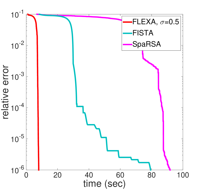
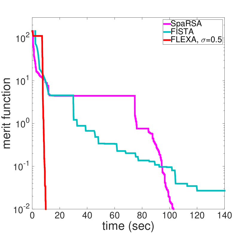
Figure 4: Nonconvex problem (13) with 1% solution sparsity: relative error vs. time (in seconds), and merit value vs. time (in seconds).

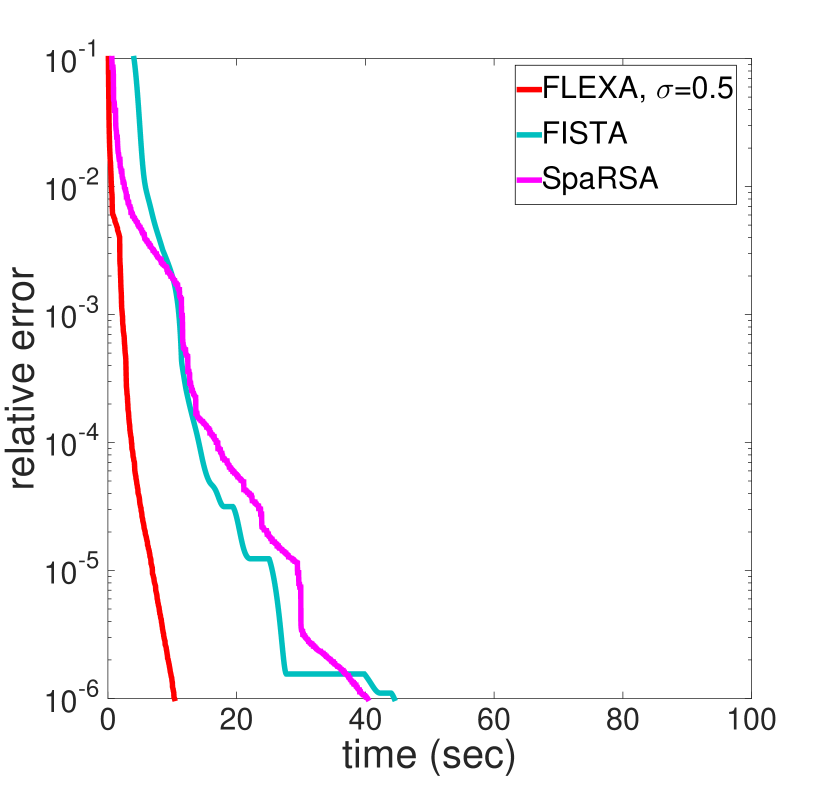
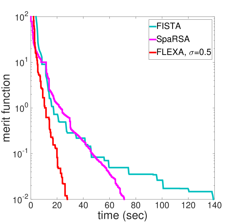
Figure 5: Nonconvex problem (13) with 10% solution sparsity:relative error vs. time (in seconds), and merit value vs. time (in seconds).

These preliminary tests seem to indicate that FLEXA performs well also on nonconvex problems.

VII Conclusions

We proposed a general algorithmic framework for the minimization of the sum of a possibly noncovex differentiable function and a possibily nonsmooth but block-separable convex one. Quite remarkably, our framework leads to different new algorithms whose degree of parallelism can be chosen by the user that also has complete control on the number of variables to update at each iterations; all the algorithms converge under the same conditions. Many well known sequential and simultaneous solution methods in the literature are just special cases of our algorithmic framework. It is remarkable that our scheme encompasses many different practical realizations and that this flexibility can be used to easily cope with different classes of problems that bring different challenges. Our preliminary tests are very promising, showing that our schemes can outperform state-of-the-art algorithms. Experiments on larger and more varied classes of problems (including those listed in Sec. II) are the subject of current research. Among the topics that should be further studied, one key issue is the right initial choice and and subsequent tuning of the $\tau_{i}$. These parameters to a certaine extent determine the lenght of the shift at each iteration and play a crucial role in establishing the quality of the results.

VIII Acknowledgments

The authors are very grateful to Loris Cannelli and Paolo Scarponi for their invaluable help in developing the C++ code of the simulated algorithms.

The work of Facchinei was supported by the MIUR project PLATINO (Grant Agreement n. PON01_01007). The work of Scutari was supported by the USA National Science Foundation under Grants CMS 1218717 and CAREER Award No. 1254739.

Appendix A Appendix: Proof of Theorem 1 and 2

We first introduce some preliminary results instrumental to prove both Theorem 1 and Theorem 2. Hereafter, for notational simplicity, we will omit the dependence of $\widehat{\mathbf{x}}(\mathbf{y},\boldsymbol{\tau})$ on $\boldsymbol{\tau}$ and write $\widehat{\mathbf{x}}(\mathbf{y})$. Given $S\subseteq\mathcal{N}$ and $\mathbf{x}\triangleq(x_{i})_{i=1}^{N}$, we will also denote by $(\mathbf{x})_{S}$ (or interchangeably $\mathbf{x}_{S}$) the vector whose component $i$ is equal to $x_{i}$ if $i\in S$, and zero otherwise.

A-A Intermediate results

Lemma 7.

Let $H(\mathbf{x};\mathbf{y})\triangleq\sum_{i}h_{i}(\mathbf{x}_{i};\mathbf{y})$. Then, the following hold:

(i) $H(\mathbf{\bullet};\mathbf{y})$ is uniformly strongly convex on $X$ with constant $c_{\boldsymbol{{\tau}}}>0$, i.e.,

$$\begin{array}[]{l}\left(\mathbf{x}-\mathbf{w}\right)^{T}\left(\nabla_{\mathbf{x}}H\left(\mathbf{x};\mathbf{y}\right)-\nabla_{\mathbf{x}}H\left(\mathbf{w};\mathbf{y}\right)\right)\geq c_{{\boldsymbol{\tau}}}\left\|\mathbf{x}-\mathbf{w}\right\|^{2}\end{array},$$ (14)

for all $\mathbf{x},\mathbf{w}\in X$ and given $\mathbf{y}\in X$;

(ii) $\nabla_{\mathbf{x}}H(\mathbf{x};\mathbf{\bullet})$ is uniformly Lipschitz continuous on $X$, i.e., there exists a $0<L_{\nabla_{H}}<\infty$ independent on $\mathbf{x}$ such that

$$\begin{array}[]{l}\left\|\nabla_{\mathbf{x}}H\left(\mathbf{x};\mathbf{y}\right)-\nabla_{\mathbf{x}}H\left(\mathbf{x};\mathbf{w}\right)\right\|\end{array}\leq\,L_{\nabla H}\,\left\|\mathbf{y}-\mathbf{w}\right\|,$$ (15)

for all $\mathbf{y},\mathbf{w}\in X$ and given $\mathbf{x}\in X$.

Proposition 8.

Consider Problem (1) under A1-A6. Then the mapping $X\ni\mathbf{y}\mapsto\widehat{\mathbf{x}}(\mathbf{y})$ has the following properties:

(a) $\widehat{\mathbf{x}}(\mathbf{\bullet})$ is Lipschitz continuous on $X$, i.e., there exists a positive constant $\hat{{L}}$ such that

$$\left\|\widehat{\mathbf{x}}(\mathbf{y})-\widehat{\mathbf{x}}(\mathbf{z})\right\|\leq\,\hat{{L}}\,\left\|\mathbf{y}-\mathbf{z}\right\|,\quad\forall\mathbf{y},\mathbf{z}\in X;\vspace{-0.3cm}$$ (16)

(b) the set of the fixed-points of $\widehat{\mathbf{x}}(\mathbf{\bullet})$ coincides with the set of stationary solutions of Problem (1); therefore $\widehat{\mathbf{x}}(\bullet)$ has a fixed-point;

(c) for every given $\mathbf{y}\in X$ and for any set $S\subseteq{\cal N}$,

$$\left(\widehat{\mathbf{x}}(\mathbf{y})-\mathbf{y}\right)_{S}^{T}\,\nabla_{\mathbf{x}}F(\mathbf{y})_{S}+ \sum_{i\in S}g_{i}(\widehat{\mathbf{x}}_{i}(\mathbf{y}))-\sum_{i\in S}g_{i}(\mathbf{y}_{i})$$ (17)

$$\leq-c_{\tau}\,\left\|(\widehat{\mathbf{x}}(\mathbf{y})-\mathbf{y})_{S}\right\|^{2},\vspace{-0.3cm}\vspace{-0.4cm}$$

with $c_{\tau}\triangleq q\,\min_{i}\tau_{i}$.

Proof.

We prove the proposition in the following order: (c), (a), (b).

(c): Given $\mathbf{y}\in X$, by definition, each $\widehat{\mathbf{x}}_{i}(\mathbf{y})$ is the unique solution of problem (4); then it is not difficult to see that the following holds: for all $\mathbf{z}_{i}\in X_{i}$,

$$\left(\mathbf{z}_{i}-\widehat{\mathbf{x}}_{i}(\mathbf{y})\right)^{T}\nabla_{\mathbf{x}_{i}}h_{i}(\widehat{\mathbf{x}}_{i}(\mathbf{y});\mathbf{y})+g_{i}(\mathbf{z}_{i})-g_{i}(\widehat{\mathbf{x}}_{i}(\mathbf{y}))\geq 0.$$ (18)

Summing and subtracting $\nabla_{\mathbf{x}_{i}}P_{i}\left(\mathbf{y}_{i};\,\mathbf{y}\right)$ in (18), choosing $\mathbf{z}_{i}=\mathbf{y}_{i}$, and using P2, we get

$$\begin{array}[t]{l}\left(\mathbf{y}_{i}-\widehat{\mathbf{x}}_{i}(\mathbf{y})\right)^{T}\left(\nabla_{\mathbf{x}_{i}}P_{i}\!\left(\widehat{\mathbf{x}}_{i}(\mathbf{y});\,\mathbf{y}\right)-\nabla_{\mathbf{x}_{i}}P_{i}\!\left(\mathbf{y}_{i};\,\mathbf{y}\right)\right)\vskip 3.0pt plus 1.0pt minus 1.0pt\\ \quad+\left(\mathbf{y}_{i}-\widehat{\mathbf{x}}_{i}(\mathbf{y})\right)^{T}\nabla_{\mathbf{x}_{i}}F(\mathbf{y})\vskip 3.0pt plus 1.0pt minus 1.0pt+g_{i}(\mathbf{y}_{i})-g_{i}(\widehat{\mathbf{x}}_{i}(\mathbf{y}))\\ \quad-\tau_{i}\,(\widehat{\mathbf{x}}_{i}(\mathbf{y})-\mathbf{y}_{i})^{T}\,\mathbf{Q}_{i}(\mathbf{y})\,(\widehat{\mathbf{x}}_{i}(\mathbf{y})-\mathbf{y}_{i})\geq 0,\end{array}$$ (19)

for all $i\in\mathcal{N}$. Observing that the term on the first line of (19) is non positive and using P1, we obtain

$$\left(\mathbf{y}_{i}-\widehat{\mathbf{x}}_{i}(\mathbf{y})\right)^{T}\nabla_{\mathbf{x}_{i}}F(\mathbf{y})+g_{i}(\mathbf{y}_{i})-g_{i}(\widehat{\mathbf{x}}_{i}(\mathbf{y}))$$

$$\,\geq c_{\boldsymbol{\tau}}\left\|\widehat{\mathbf{x}}_{i}(\mathbf{y})-\mathbf{y}_{i}\right\|^{2},$$

for all $i\in\mathcal{N}$. Summing over $i\in S$ we get (17).

(a): We use the notation introduced in Lemma 7. Given $\mathbf{y},\mathbf{z}\in X$, by optimality and (18), we have, for all $\mathbf{v}$ and $\mathbf{w}$ in $X$

$$\begin{array}[]{l}\left(\mathbf{v}-\widehat{\mathbf{x}}(\mathbf{y})\right)^{T}\nabla_{\mathbf{x}}H\left(\widehat{\mathbf{x}}(\mathbf{y});\mathbf{y}\right)+G(\mathbf{v})-G(\widehat{\mathbf{x}}(\mathbf{y}))\geq 0\\ \left(\mathbf{w}-\widehat{\mathbf{x}}(\mathbf{z})\right)^{T}\nabla_{\mathbf{x}}H\left(\widehat{\mathbf{x}}(\mathbf{z});\mathbf{z}\right)+G(\mathbf{w})-G(\widehat{\mathbf{x}}(\mathbf{z}))\geq 0.\end{array}$$

Setting $\mathbf{v}=\widehat{\mathbf{x}}(\mathbf{z})$ and $\mathbf{w}=\widehat{\mathbf{x}}(\mathbf{y})$, summing the two inequalities above, and adding and subtracting $\nabla_{\mathbf{x}}H\left(\widehat{\mathbf{x}}(\mathbf{y});\mathbf{z}\right)$, we obtain:

$$\begin{array}[]{l}\left(\widehat{\mathbf{x}}(\mathbf{z})-\widehat{\mathbf{x}}(\mathbf{y})\right)^{T}\left(\nabla_{\mathbf{x}}H\left(\widehat{\mathbf{x}}(\mathbf{z});\mathbf{z}\right)-\nabla_{\mathbf{x}}H\left(\widehat{\mathbf{x}}(\mathbf{y});\mathbf{z}\right)\right)\\ \leq\left(\widehat{\mathbf{x}}(\mathbf{y})-\widehat{\mathbf{x}}(\mathbf{z})\right)^{T}\left(\nabla_{\mathbf{x}}H\left(\widehat{\mathbf{x}}(\mathbf{y});\mathbf{z}\right)-\nabla_{\mathbf{x}}H\left(\widehat{\mathbf{x}}(\mathbf{y});\mathbf{y}\right)\right).\end{array}$$ (20)

Using (14) we can lower bound the left-hand-side of (20) as

$$\begin{array}[]{l}\left(\widehat{\mathbf{x}}(\mathbf{z})-\widehat{\mathbf{x}}(\mathbf{y})\right)^{T}\left(\nabla_{\mathbf{x}}H\left(\widehat{\mathbf{x}}(\mathbf{z});\mathbf{z}\right)-\nabla_{\mathbf{x}}H\left(\widehat{\mathbf{x}}(\mathbf{y});\mathbf{z}\right)\right)\\ \,\,\geq c_{{\boldsymbol{\tau}}}\left\|\widehat{\mathbf{x}}(\mathbf{z})-\widehat{\mathbf{x}}(\mathbf{y})\right\|^{2},\end{array}$$ (21)

whereas the right-hand-side of (20) can be upper bounded as

$$\begin{array}[]{l}\left(\widehat{\mathbf{x}}(\mathbf{y})-\widehat{\mathbf{x}}(\mathbf{z})\right)^{T}\left(\nabla_{\mathbf{x}}H\left(\widehat{\mathbf{x}}(\mathbf{y});\mathbf{z}\right)-\nabla_{\mathbf{x}}H\left(\widehat{\mathbf{x}}(\mathbf{y});\mathbf{y}\right)\right)\\ \,\,\leq\,L_{\nabla H}\,\left\|\widehat{\mathbf{x}}(\mathbf{y})-\widehat{\mathbf{x}}(\mathbf{z})\right\|\,\left\|\mathbf{y}-\mathbf{z}\right\|,\end{array}$$ (22)

where the inequality follows from the Cauchy-Schwartz inequality and (15). Combining (20), (21), and (22), we obtain the desired Lipschitz property of $\widehat{\mathbf{x}}(\bullet)$.

(b): Let $\mathbf{x}^{\star}\in X$ be a fixed point of $\widehat{\mathbf{x}}(\mathbf{y})$, that is $\mathbf{x}^{\star}=\widehat{\mathbf{x}}(\mathbf{x}^{\star})$. Each $\widehat{\mathbf{x}}_{i}(\mathbf{y})$ satisfies (18) for any given $\mathbf{y}\in X$. For some $\boldsymbol{\xi}_{i}\in\partial g_{i}(\mathbf{x}^{*})$, setting $\mathbf{y}=\mathbf{x}^{\star}$ and using $\mathbf{x}^{\star}=\widehat{\mathbf{x}}(\mathbf{x}^{\star})$ and the convexity of $g_{i}$, (18) reduces to

$$\left(\mathbf{z}_{i}-\mathbf{x}_{i}^{\star}\right)^{T}(\nabla_{\mathbf{x}_{i}}F(\mathbf{x}^{\star})+\boldsymbol{\xi}_{i})\geq 0,$$ (23)

for all $\mathbf{z}_{i}\in X_{i}$ and $i\in\mathcal{N}$. Taking into account the Cartesian structure of $X$, the separability of $G$, and summing (23) over $i\in\mathcal{N}$, we obtain $\begin{array}[t]{l}\left(\mathbf{z}-\mathbf{x}^{\star}\right)^{T}(\nabla_{\mathbf{x}}F(\mathbf{x}^{\star})+\boldsymbol{\xi})\geq 0,\end{array}$ for all $\mathbf{z}\in X,$ with $\mathbf{z}\triangleq(\mathbf{z}_{i})_{i=1}^{N}$ and $\boldsymbol{\xi}\triangleq(\boldsymbol{\xi}_{i})_{i=1}^{N}\in\partial G(\mathbf{x}^{*})$; therefore $\mathbf{x}^{\star}$ is a stationary solution of (1).

The converse holds because i) $\widehat{\mathbf{x}}(\mathbf{x}^{\star})$ is the unique optimal solution of (4) with $\mathbf{y}=\mathbf{x}^{\star}$, and ii) $\mathbf{x}^{\star}$ is also an optimal solution of (4), since it satisfies the minimum principle.∎

Lemma 9.

[42, Lemma 3.4, p.121] Let $\{X^{k}\}$, $\{Y^{k}\}$, and $\{Z^{k}\}$ be three sequences of numbers such that $Y^{k}\geq 0$ for all $k$. Suppose that

$$X^{k+1}\leq X^{k}-Y^{k}+Z^{k},\quad\forall k=0,1,\ldots$$

and $\sum_{k=0}^{\infty}Z^{k}<\infty$. Then either $X^{k}\rightarrow-\infty$ or else $\{X^{k}\}$ converges to a finite value and $\sum_{k=0}^{\infty}Y^{k}<\infty$.

Lemma 10.

Let $\{\mathbf{x}^{k}\}$ be the sequence generated by Algorithm 1. Then, there is a positive constant $\tilde{c}$ such that the following holds: for all $k\geq 1$,

$$\begin{array}[]{ll}\left(\nabla_{\mathbf{x}}F(\mathbf{x}^{k})\right)^{T}_{\tiny{S^{k}}}\left(\widehat{\mathbf{x}}(\mathbf{x}^{k})-\mathbf{x}^{k}\right)_{\tiny{S^{k}}}+\displaystyle{\sum_{i\in S^{k}}}g_{i}(\widehat{\mathbf{x}}_{i}(\mathbf{x}^{k}))\vskip 6.0pt plus 2.0pt minus 2.0pt\\ \quad\quad\quad\quad\quad-\displaystyle{\sum_{i\in S^{k}}}g_{i}(\mathbf{x}_{i}^{k})\leq-\tilde{c}\,\|\widehat{\mathbf{x}}(\mathbf{x}^{k})-\mathbf{x}^{k}\|^{2}.\end{array}$$ (24)

Proof.

Let $j_{k}$ be an index in $S^{k}$ such that $E_{j_{k}}(\mathbf{x}^{k})\geq\rho\max_{i}E_{i}(\mathbf{x}^{k})$ (Step 2 of Algorithm 1). Then, using the aforementioned bound and (5), it is easy to check that the following chain of inequalities holds:

$$\bar{s}_{j_{k}}\|\widehat{\mathbf{x}}_{S^{k}}(\mathbf{x}^{k})-\mathbf{x}^{k}_{S^{k}}\| \geq\bar{s}_{j_{k}}\|\widehat{\mathbf{x}}_{j_{k}}(\mathbf{x}^{k})-\mathbf{x}^{k}_{j_{k}}\|$$

$$\geq E_{j_{k}}(\mathbf{x}^{k})$$

$$\geq\rho\max_{i}E_{i}(\mathbf{x}^{k})$$

$$\geq\left(\rho\min_{i}\underline{s}_{i}\right)\left(\max_{i}\{\|\widehat{\mathbf{x}}_{i}(\mathbf{x}^{k})-\mathbf{x}^{k}_{i}\|\}\right)$$

$$\geq\left(\frac{\rho\min_{i}\underline{s}_{i}}{N}\right)\|\widehat{\mathbf{x}}(\mathbf{x}^{k})-\mathbf{x}^{k}\|.$$

Hence we have for any $k$,

$$\|\widehat{\mathbf{x}}_{S^{k}}(\mathbf{x}^{k})-\mathbf{x}^{k}_{S^{k}}\|\geq\left(\frac{\rho\min_{i}\underline{s}_{i}}{N\bar{s}_{j_{k}}}\right)\|\widehat{\mathbf{x}}(\mathbf{x}^{k})-\mathbf{x}^{k}\|.$$ (25)

Invoking now Proposition 8(c) with $S=S^{k}$ and $\mathbf{y}=\mathbf{x}^{k}$, and using (25), (24) holds true, with $\tilde{c}\triangleq c_{\tau}\left(\frac{\rho\min_{i}\underline{s}_{i}}{N\max_{j}\bar{s}_{j}}\right)^{2}$. ∎

A-B Proof of Theorem 1

We are now ready to prove the theorem. For any given $k\geq 0$, the Descent Lemma [33] yields

$$\begin{array}[]{lll}F\left(\mathbf{x}^{k+1}\right)&\leq&F\left(\mathbf{x}^{k}\right)+\gamma^{k}\,\nabla_{\mathbf{x}}F\left(\mathbf{x}^{k}\right)^{T}\left(\widehat{\mathbf{z}}^{k}-\mathbf{x}^{k}\right)\vskip 3.0pt plus 1.0pt minus 1.0pt\\ &&+\dfrac{\left(\gamma^{k}\right)^{2}{L_{\nabla F}}}{2}\,\left\|\widehat{\mathbf{z}}^{k}-\mathbf{x}^{k}\right\|^{2},\end{array}$$ (26)

with $\widehat{\mathbf{z}}^{k}\triangleq(\widehat{\mathbf{z}}_{i}^{k})_{i=1}^{N}$ and $\mathbf{z}^{k}\triangleq(\mathbf{z}_{i}^{k})_{i=1}^{N}$ defined in Step 2 and 3 (Algorithm III). Observe that

$$\begin{array}[]{rcl}\left\|\widehat{\mathbf{z}}^{k}-\mathbf{x}^{k}\right\|^{2}&\leq&\left\|\mathbf{z}^{k}-\mathbf{x}^{k}\right\|^{2}\\ &\leq&2\left\|\widehat{\mathbf{x}}(\mathbf{x}^{k})-\mathbf{x}^{k}\right\|^{2}\\ &&+2\sum_{i\in\cal N}\left\|\mathbf{z}_{i}^{k}-\widehat{\mathbf{x}}_{i}(\mathbf{x}^{k})\right\|^{2}\\ &\leq&2\left\|\widehat{\mathbf{x}}(\mathbf{x}^{k})-\mathbf{x}^{k}\right\|^{2}+2\sum_{i\in\cal N}(\varepsilon_{i}^{k})^{2},\end{array}$$ (27)

where the first inequality follows from the definition of $\mathbf{z}^{k}$ and $\widehat{\mathbf{z}}^{k}$, and in the last inequality we used $\left\|\mathbf{z}_{i}^{k}-\widehat{\mathbf{x}}_{i}(\mathbf{x}^{k})\right\|\leq\varepsilon_{i}^{k}$.

Denoting by $\overline{S}^{k}$ the complement of $S$, we also have, for all $k$,

$$\begin{array}[]{l}\nabla_{\mathbf{x}}F\left(\mathbf{x}^{k}\right)^{T}\left(\widehat{\mathbf{z}}^{k}-\mathbf{x}^{k}\right)\vskip 3.0pt plus 1.0pt minus 1.0pt\\ \qquad\qquad=\nabla_{\mathbf{x}}F\left(\mathbf{x}^{k}\right)^{T}\left(\widehat{\mathbf{z}}^{k}-\widehat{\mathbf{x}}(\mathbf{x}^{k})+\widehat{\mathbf{x}}(\mathbf{x}^{k})-\mathbf{x}^{k}\right)\vskip 3.0pt plus 1.0pt minus 1.0pt\\ \qquad\qquad=\nabla_{\mathbf{x}}F\left(\mathbf{x}^{k}\right)^{T}_{S^{k}}(\mathbf{z}^{k}-\widehat{\mathbf{x}}(\mathbf{x}^{k}))_{S^{k}}\vskip 3.0pt plus 1.0pt minus 1.0pt\\ \qquad\qquad\quad+\nabla_{\mathbf{x}}F\left(\mathbf{x}^{k}\right)^{T}_{\overline{S}^{k}}(\mathbf{x}^{k}-\widehat{\mathbf{x}}(\mathbf{x}^{k}))_{\overline{S}^{k}}\vskip 3.0pt plus 1.0pt minus 1.0pt\\ \qquad\qquad\quad+\nabla_{\mathbf{x}}F\left(\mathbf{x}^{k}\right)^{T}_{S^{k}}(\widehat{\mathbf{x}}(\mathbf{x}^{k})-\mathbf{x}^{k})_{S^{k}}\vskip 3.0pt plus 1.0pt minus 1.0pt\\ \qquad\qquad\quad+\nabla_{\mathbf{x}}F\left(\mathbf{x}^{k}\right)^{T}_{\overline{S}^{k}}(\widehat{\mathbf{x}}(\mathbf{x}^{k})-\mathbf{x}^{k})_{\overline{S}^{k}}\vskip 3.0pt plus 1.0pt minus 1.0pt\\ \qquad\qquad=\nabla_{\mathbf{x}}F\left(\mathbf{x}^{k}\right)^{T}_{S^{k}}(\mathbf{z}^{k}-\widehat{\mathbf{x}}(\mathbf{x}^{k}))_{S^{k}}\vskip 3.0pt plus 1.0pt minus 1.0pt\\ \qquad\qquad+\nabla_{\mathbf{x}}F\left(\mathbf{x}^{k}\right)^{T}_{S^{k}}(\widehat{\mathbf{x}}(\mathbf{x}^{k})-\mathbf{x}^{k})_{S^{k}},\end{array}$$ (28)

where in the second equality we used the definition of $\widehat{\mathbf{z}}^{k}$ and of the set $S^{k}$. Now, using (28) and Lemma 10, we can write

$$\begin{array}[]{rl}\lx@intercol\nabla_{\mathbf{x}}F\left(\mathbf{x}^{k}\right)^{T}\left(\widehat{\mathbf{z}}^{k}-\mathbf{x}^{k}\right)+\sum_{i\in S^{k}}g_{i}(\widehat{\mathbf{z}}_{i}^{k})-\sum_{i\in S^{k}}g_{i}(\mathbf{x}^{k}_{i})\hfil\lx@intercol\\[3.00003pt] =&\nabla_{\mathbf{x}}F\left(\mathbf{x}^{k}\right)^{T}\left(\widehat{\mathbf{z}}^{k}-\mathbf{x}^{k}\right)+\sum_{i\in S^{k}}g_{i}(\widehat{\mathbf{x}}_{i}(\mathbf{x}^{k}))\\[3.00003pt] &-\sum_{i\in S^{k}}g_{i}(\mathbf{x}^{k}_{i})+\sum_{i\in S^{k}}g_{i}(\widehat{\mathbf{z}}_{i}^{k})-\sum_{i\in S^{k}}g_{i}(\widehat{\mathbf{x}}_{i}(\mathbf{x}^{k}))\end{array}$$ (29)

$$\begin{array}[]{rl}\leq&-\tilde{c}\left\|\widehat{\mathbf{x}}(\mathbf{x}^{k})-\mathbf{x}^{k}\right\|^{2}+\sum_{i\in S^{k}}\varepsilon_{i}^{k}\left\|\nabla_{\mathbf{x}_{i}}F(\mathbf{x}^{k})\right\|\\[3.00003pt] &+L_{G}\sum_{i\in S^{k}}\varepsilon_{i}^{k},\end{array}$$ (30)

where $L_{G}$ is a (global) Lipschitz constant for (all) $g_{i}$.
Finally, from the definition of $\widehat{\mathbf{z}}^{k}$ and of the set $S^{k}$, we have for all $k$,

$$\begin{array}[]{l}V(\mathbf{x}^{k+1})=F(\mathbf{x}^{k+1})+\sum_{{i\in\cal N}}g_{i}(\mathbf{x}_{i}^{k+1})\\[3.00003pt] =F(\mathbf{x}^{k+1})+\sum_{i\in{\cal N}}g_{i}(\mathbf{x}_{i}^{k}+\gamma^{k}(\widehat{\mathbf{z}}^{k}_{i}-\mathbf{x}_{i}^{k}))\\[3.00003pt] \leq F(\mathbf{x}^{k+1})+\sum_{i\in\cal N}g_{i}(\mathbf{x}^{k}_{i})+\gamma^{k}\left(\sum_{i\in S^{k}}(g_{i}(\widehat{\mathbf{z}}^{k}_{i})-g_{i}(\mathbf{x}^{k}_{i}))\right)\\[3.00003pt] \leq V\left(\mathbf{x}^{k}\right)-\gamma^{k}\left(\tilde{c}-\gamma^{k}{L_{\nabla F}}\right)\left\|\widehat{\mathbf{x}}(\mathbf{x}^{k})-\mathbf{x}^{k}\right\|^{2}+T^{k},\end{array}$$ (31)

where in the first inequality we used the the convexity of the $g_{i}$’s, whereas the second one follows from (26), (27) and (30), with

$$T^{k}\triangleq\gamma^{k}\,\sum_{i\in S^{k}}\varepsilon_{i}^{k}\left(L_{G}+\left\|\nabla_{\mathbf{x}_{i}}F(\mathbf{x}^{k})\right\|\right)+\left(\gamma^{k}\right)^{2}{L_{\nabla F}}\,\sum_{i\in\cal N}(\varepsilon_{i}^{k})^{2}.$$

Using assumption (iv), we can bound $T^{k}$ as

$$T^{k}\leq(\gamma^{k})^{2}\left[N\alpha_{1}(\alpha_{2}L_{G}+1)+(\gamma^{k})^{2}L_{\nabla F}\left(N\alpha_{1}\alpha_{2}\right)^{2}\right],$$

which, by assumption (iii) implies $\sum_{k=0}^{\infty}T^{k}<\infty$. Since $\gamma^{k}\rightarrow 0$, it follows from (31) that there exist some positive constant $\beta_{1}$ and a sufficiently large $k$, say $\bar{{k}}$, such that

$$V(\mathbf{x}^{k+1})\leq V(\mathbf{x}^{k})-\gamma^{k}\beta_{1}\left\|\widehat{\mathbf{x}}(\mathbf{x}^{k})-\mathbf{x}^{k}\right\|^{2}+T^{k},$$ (32)

for all $k\geq\bar{{k}}$. Invoking Lemma 9 with the identifications $X^{k}=V(\mathbf{x}^{k+1})$, $Y^{k}=\gamma^{k}\beta_{1}\left\|\widehat{\mathbf{x}}(\mathbf{x}^{k})-\mathbf{x}^{k}\right\|^{2}$ and $Z^{k}=T^{k}$ while using $\sum_{k=0}^{\infty}T^{k}<\infty$, we deduce from (32) that either $\{V(\mathbf{x}^{k})\}\rightarrow-\infty$ or else $\{V(\mathbf{x}^{k})\}$ converges to a finite value and

$$\lim_{k\rightarrow\infty}\sum_{t=\bar{{k}}}^{k}\gamma^{t}\left\|\widehat{\mathbf{x}}(\mathbf{x}^{t})-\mathbf{x}^{t}\right\|^{2}<+\infty.\vspace{-0.1cm}$$ (33)

Since $V$ is coercive, $V(\mathbf{x})\geq\min_{\mathbf{y}\in X}V(\mathbf{y})>-\infty$, implying that $\{V\left(\mathbf{x}^{k}\right)\}$ is convergent; it follows from (33) and $\sum_{k=0}^{\infty}\gamma^{k}=\infty$ that $\liminf_{k\rightarrow\infty}\left\|\widehat{\mathbf{x}}(\mathbf{x}^{k})-\mathbf{x}^{k}\right\|=0.$
Using Proposition 8, we show next that $\lim_{k\rightarrow\infty}\left\|\widehat{\mathbf{x}}(\mathbf{x}^{k})-\mathbf{x}^{k}\right\|=0$; for notational simplicity we will write $\triangle\widehat{\mathbf{x}}(\mathbf{x}^{k})\triangleq\widehat{\mathbf{x}}(\mathbf{x}^{k})-\mathbf{x}^{k}$. Suppose, by contradiction, that $\limsup_{k\rightarrow\infty}\left\|\triangle\widehat{\mathbf{x}}(\mathbf{x}^{k})\right\|>0$. Then, there exists a $\delta>0$ such that $\left\|\triangle\widehat{\mathbf{x}}(\mathbf{x}^{k})\right\|>2\delta$ for infinitely many $k$ and also $\left\|\triangle\widehat{\mathbf{x}}(\mathbf{x}^{k})\right\|<\delta$ for infinitely many $k$. Therefore, one can always find an infinite set of indexes, say $\mathcal{K}$, having the following properties: for any $k\in\mathcal{K}$, there exists an integer $i_{k}>k$ such that

$$\left\|\triangle\widehat{\mathbf{x}}(\mathbf{x}^{k})\right\|<\delta, \left\|\triangle\widehat{\mathbf{x}}(\mathbf{x}^{i_{k}})\right\|>2\delta\vskip 6.0pt plus 2.0pt minus 2.0pt$$ (34)

$$\delta\leq\left\|\triangle\widehat{\mathbf{x}}(\mathbf{x}^{j})\right\|\leq 2\delta k<j<i_{k}.$$ (35)

Given the above bounds, the following holds: for all $k\in\mathcal{K}$,

$$\delta \overset{(a)}{<} \left\|\triangle\widehat{\mathbf{x}}(\mathbf{x}^{i_{k}})\right\|-\left\|\triangle\widehat{\mathbf{x}}(\mathbf{x}^{k})\right\|\vskip 6.0pt plus 2.0pt minus 2.0pt$$

$$\leq \left\|\widehat{\mathbf{x}}(\mathbf{x}^{i_{k}})-\widehat{\mathbf{x}}(\mathbf{x}^{k})\right\|+\left\|\mathbf{x}^{i_{k}}-\mathbf{x}^{k}\right\|$$

$$\overset{(b)}{\leq} (1+\hat{{L}})\left\|\mathbf{x}^{i_{k}}-\mathbf{x}^{k}\right\|$$

$$\overset{(c)}{\leq} {\color[rgb]{0,0,0}(1+\hat{{L}})\sum_{t=k}^{i_{k}-1}\gamma^{t}\left(\left\|\triangle\widehat{\mathbf{x}}(\mathbf{x}^{t})_{S^{t}}\right\|+\left\|(\mathbf{z}^{t}-\widehat{\mathbf{x}}(\mathbf{x}^{t}))_{S^{t}}\right\|\right)}\vspace{-0.3cm}$$ (36)

$$\overset{(d)}{\leq} (1+\hat{{L}})\,(2\delta+\varepsilon^{\max})\sum_{t=k}^{i_{k}-1}\gamma^{t},$$

where (a) follows from (34); (b) is due to Proposition 8(a); (c) comes from the triangle inequality, the updating rule of the algorithm and the definition of $\widehat{\mathbf{z}}^{k}$; and in (d) we used (34), (35), and $\left\|\mathbf{z}^{t}-\widehat{\mathbf{x}}(\mathbf{x}^{t})\right\|\leq\sum_{i\in\cal N}\varepsilon_{i}^{t}$, where $\varepsilon^{\max}\triangleq\max_{k}\sum_{i\in\cal N}\varepsilon_{i}^{k}<\infty$. It follows from (36) that

$$\liminf_{k\rightarrow\infty}\sum_{t=k}^{i_{k}-1}\gamma^{t}\geq\dfrac{{\delta}}{(1+\hat{{L}})(2\delta+\varepsilon^{\max})}>0.$$ (37)

We show next that (37) is in contradiction with the convergence of $\{V(\mathbf{x}^{k})\}$. To do that, we preliminary prove that, for sufficiently large $k\in\mathcal{K}$, it must be $\left\|\triangle\widehat{\mathbf{x}}(\mathbf{x}^{k})\right\|\geq\delta/2$. Proceeding as in (36), we have: for any given $k\in\mathcal{K}$,

$$\begin{array}[]{l}\left\|\triangle\widehat{\mathbf{x}}(\mathbf{x}^{k+1})\right\|-\left\|\triangle\widehat{\mathbf{x}}(\mathbf{x}^{k})\right\|\leq(1+\hat{{L}})\left\|\mathbf{x}^{k+1}-\mathbf{x}^{k}\right\|\vskip 3.0pt plus 1.0pt minus 1.0pt\\ \qquad\qquad\qquad\qquad\qquad\leq(1+\hat{{L}})\gamma^{k}\left(\left\|\triangle\widehat{\mathbf{x}}(\mathbf{x}^{k})\right\|+\varepsilon^{\max}\right).\end{array}$$

It turns out that for sufficiently large $k\in\mathcal{K}$ so that $(1+\hat{{L}})\gamma^{k}<\delta/(\delta+2\varepsilon^{\max})$, it must be

$$\left\|\triangle\widehat{\mathbf{x}}(\mathbf{x}^{k})\right\|\geq\delta/2;$$ (38)

otherwise the condition $\left\|\triangle\widehat{\mathbf{x}}(\mathbf{x}^{k+1})\right\|\geq\delta$ would be violated [cf. (35)]. Hereafter we assume without loss of generality that (38) holds for all $k\in\mathcal{K}$ (in fact, one can alway restrict $\{\mathbf{x}^{k}\}_{k\in\mathcal{K}}$ to a proper subsequence).

We can show now that (37) is in contradiction with the convergence of $\{V(\mathbf{x}^{k})\}$. Using (32) (possibly over a subsequence), we have: for sufficiently large $k\in\mathcal{K}$,

$$V(\mathbf{x}^{i_{k}}) \leq V(\mathbf{x}^{k})-\beta_{2}\sum_{t=k}^{i_{k}-1}\gamma^{t}\left\|\triangle\widehat{\mathbf{x}}(\mathbf{x}^{t})\right\|^{2}+\sum_{t=k}^{i_{k}-1}T^{t}$$ (39)

$$\overset{(a)}{<} V(\mathbf{x}^{k})-\beta_{2}(\delta^{2}/4)\sum_{t=k}^{i_{k}-1}\gamma^{t}+\sum_{t=k}^{i_{k}-1}T^{t}$$

where in (a) we used (35) and (38), and $\beta_{2}$ is some positive constant. Since $\{V(\mathbf{x}^{k})\}$ converges and $\sum_{k=0}^{\infty}T^{k}<\infty$, (39) implies $\lim_{\mathcal{K}\ni k\rightarrow\infty}\,\sum_{t=k}^{i_{k}-1}\gamma^{t}=0,$ which contradicts (37). Finally, since the sequence $\{\mathbf{x}^{k}\}$ is bounded [by the coercivity of $V$ and the convergence of $\{V(\mathbf{x}^{k})\}$], it has at least one limit point $\bar{{\mathbf{x}}}$, that belongs to $X$. By the continuity of $\widehat{\mathbf{x}}(\bullet)$ [Proposition 8(a)] and $\lim_{k\rightarrow\infty}\left\|\widehat{\mathbf{x}}(\mathbf{x}^{k})-\mathbf{x}^{k}\right\|=0$, it must be $\widehat{\mathbf{x}}(\bar{{\mathbf{x}}})=\bar{{\mathbf{x}}}$. By Proposition 8(b) $\bar{{\mathbf{x}}}$ is a stationary solution of Problem (1). As a final remark, note that if $\varepsilon_{i}^{k}=0$ for every $i$ and for every $k$ large enough, i.e., if eventually $\widehat{\mathbf{x}}(\mathbf{x}^{k})$ is computed exactly, there is no need to assume that $G$ is globally Lipschitz. In fact in (30) the term containing $L_{G}$ disappears, all $T^{k}$ are zero and all the subsequent derivations hold independent of the Lipschitzianity of $G$. $\square$

A-C Proof of Theorem 2

We show next that Algorithm III-A is just an instance of the inexact Jacobi scheme described in Algorithm III satisfying the convergence conditions in Theorem 1; which proves Theorem 2. It is not difficult to see that this boils down to proving that, for all $p\in P$ and $i\in I_{p}$, the sequence $\mathbf{z}_{pi}^{k}$ in Step 2a) of Algorithm III-A satisfies

$$\|\mathbf{z}_{pi}^{k}-\widehat{{\mathbf{x}}}_{pi}(\mathbf{x}^{k})\|\leq\tilde{\varepsilon}_{pi}^{k},$$ (40)

for some $\{\tilde{\varepsilon}_{pi}^{k}\}$ such that $\sum_{n}\tilde{\varepsilon}_{pi}^{k}\,\gamma^{k}<\infty$. The following holds for the LHS of (40):

$$\begin{array}[]{l}\!\!\!\!\|\mathbf{z}_{pi}^{k}-\widehat{\mathbf{x}}_{pi}(\mathbf{x}^{k})\|\leq\|\widehat{\mathbf{x}}_{pi}(\mathbf{x}_{pi<}^{k+1},\mathbf{x}_{pi\geq}^{k},\mathbf{x}_{-p}^{k})-\widehat{\mathbf{x}}_{pi}(\mathbf{x}^{k})\|\\[5.0pt] \quad\quad\quad\quad\quad\quad\,\quad+\,\|\mathbf{z}_{pi}^{k}-\widehat{\mathbf{x}}_{pi}(\mathbf{x}_{pi<}^{k+1},\mathbf{x}_{pi\geq}^{k},\mathbf{x}_{-p}^{k})\|\vskip 3.0pt plus 1.0pt minus 1.0pt\\[5.0pt] \quad\overset{(a)}{\leq}\|\widehat{\mathbf{x}}_{pi}(\mathbf{x}_{pi<}^{k+1},\mathbf{x}_{pi\geq}^{k},\mathbf{x}_{-p}^{k})-\widehat{\mathbf{x}}_{pi}(\mathbf{x}^{k})\|+{\varepsilon}_{pi}^{k}\\[5.0pt] \quad\overset{(b)}{\leq}\hat{{L}}\,\|\mathbf{x}_{pi<}^{k+1}-\mathbf{x}_{pi<}^{k}\|+{\varepsilon}_{pi}^{k}\vskip 3.0pt plus 1.0pt minus 1.0pt\\[5.0pt] \quad\overset{(c)}{=}\hat{{L}}\gamma^{k}\left\|\left(\mathbf{z}_{pi<}^{k}-\mathbf{x}_{pi<}^{k}\right)\right\|+{\varepsilon}_{pi}^{k}\\[5.0pt] \quad\leq\hat{{L}}\gamma^{k}\left(\sum_{j=1}^{i-1}(\|\mathbf{z}^{k}_{pj}-\widehat{\mathbf{x}}_{pj}(\mathbf{x}^{k})\|+\|\widehat{\mathbf{x}}_{pj}(\mathbf{x}^{k})-\mathbf{x}^{k}_{pj}\|)\right)\\[5.0pt] \quad\quad+\,{\varepsilon}_{pi}^{k}\\[5.0pt] \quad\overset{(d)}{\leq}\hat{{L}}\gamma^{k}\sum_{j=1}^{i-1}{\varepsilon}_{pj}^{k}+\hat{{L}}\gamma^{k}\left(\dfrac{L_{G}+\beta}{c_{\boldsymbol{\tau}}}\right)+{\varepsilon}_{pi}^{k}\triangleq\tilde{\varepsilon}_{pi}^{k},\end{array}$$ (41)

where (a) follows from the error bound in Step 2a) of Algorithm III-A; in (b) we used Proposition 8a); (c) is due to Step 2b); and (d) follows from $\|\widehat{\mathbf{x}}_{pj}(\mathbf{x}^{k})-\mathbf{x}^{k}_{pj}\|\leq(L_{G}+\|\nabla_{\mathbf{x}_{pi}}F(\mathbf{x}^{k})\|)/c_{\boldsymbol{\tau}}$ and $\|\nabla_{\mathbf{x}_{pi}}F(\mathbf{x}^{k})\|\leq\beta$ for some $0<\beta<\infty$. It turns out that (40) is satisfied choosing $\tilde{\varepsilon}_{pi}^{k}$ as defined in the last inequality of (41).

References

- [1] F. Facchinei, S. Sagratella, and G. Scutari, “Flexible parallel algorithms for big data optimization,” in Proc. of the IEEE 2014 International Conference on Acoustics, Speech, and Signal Processing (ICASSP 2014), Florence, Italy, May 4-9,. [Online]. Available: http://arxiv.org/abs/1311.2444
- [2] R. Tibshirani, “Regression shrinkage and selection via the lasso,” Journal of the Royal Statistical Society. Series B (Methodological), pp. 267–288, 1996.
- [3] Z. Qin, K. Scheinberg, and D. Goldfarb, “Efficient block-coordinate descent algorithms for the group lasso,” Mathematical Programming Computation, vol. 5, pp. 143–169, June 2013.
- [4] A. Rakotomamonjy, “Surveying and comparing simultaneous sparse approximation (or group-lasso) algorithms,” Signal processing, vol. 91, no. 7, pp. 1505–1526, July 2011.
- [5] G.-X. Yuan, K.-W. Chang, C.-J. Hsieh, and C.-J. Lin, “A comparison of optimization methods and software for large-scale l1-regularized linear classification,” The Journal of Machine Learning Research, vol. 9999, pp. 3183–3234, 2010.
- [6] R. H. Byrd, J. Nocedal, and F. Oztoprak, “An Inexact Successive Quadratic Approximation Method for Convex L-1 Regularized Optimization,” arXiv preprint arXiv:1309.3529, 2013.
- [7] K. Fountoulakis and J. Gondzio, “A Second-Order Method for Strongly Convex L1-Regularization Problems,” arXiv preprint arXiv:1306.5386, 2013.
- [8] I. Necoara and D. Clipici, “Efficient parallel coordinate descent algorithm for convex optimization problems with separable constraints: application to distributed MPC,” Journal of Process Control, vol. 23, no. 3, pp. 243–253, March 2013.
- [9] Y. Nesterov, “Gradient methods for minimizing composite functions,” Mathematical Programming, vol. 140, pp. 125–161, August 2013.
- [10] P. Tseng and S. Yun, “A coordinate gradient descent method for nonsmooth separable minimization,” Mathematical Programming, vol. 117, no. 1-2, pp. 387–423, March 2009.
- [11] A. Beck and M. Teboulle, “A fast iterative shrinkage-thresholding algorithm for linear inverse problems,” SIAM Journal on Imaging Sciences, vol. 2, no. 1, pp. 183–202, Jan. 2009.
- [12] S. J. Wright, R. D. Nowak, and M. A. Figueiredo, “Sparse reconstruction by separable approximation,” IEEE Trans. on Signal Processing, vol. 57, no. 7, pp. 2479–2493, July 2009.
- [13] Z. Peng, M. Yan, and W. Yin, “Parallel and distributed sparse optimization,” in Signals, Systems and Computers, 2013 Asilomar Conference on. IEEE, 2013, pp. 659–646.
- [14] M. Razaviyayn, M. Hong, and Z.-Q. Luo, “A unified convergence analysis of block successive minimization methods for nonsmooth optimization,” SIAM Journal on Optimization, vol. 23, no. 2, pp. 1126–1153, 2013.
- [15] P. L. Bühlmann, S. A. van de Geer, and S. Van de Geer, Statistics for high-dimensional data. Springer, 2011.
- [16] S. Sra, S. Nowozin, and S. J. Wright, Eds., Optimization for Machine Learning, ser. Neural Information Processing. Cambridge, Massachusetts: The MIT Press, Sept. 2011.
- [17] F. Bach, R. Jenatton, J. Mairal, and G. Obozinski, Optimization with Sparsity-inducing Penalties. Foundations and Trends® in Machine Learning, Now Publishers Inc, Dec. 2011.
- [18] Y. Li and S. Osher, “Coordinate descent optimization for minimization with application to compressed sensing; a greedy algorithm,” Inverse Probl. Imaging, vol. 3, no. 3, pp. 487–503, 2009.
- [19] I. S. Dhillon, P. K. Ravikumar, and A. Tewari, “Nearest neighbor based greedy coordinate descent,” in Advances in Neural Information Processing Systems 24, J. Shawe-Taylor, R. Zemel, P. Bartlett, F. Pereira, and K. Weinberger, Eds. Curran Associates, Inc., 2011, pp. 2160–2168.
- [20] C. Scherrer, A. Tewari, M. Halappanavar, and D. Haglin, “Feature clustering for accelerating parallel coordinate descent,” in Proc. of the 26th Annual Conference on Neural Information Processing Systems (NIPS), Lake Tahoe, NV, USA, Dec. 3–6 2012, pp. 28–36.
- [21] G. Scutari, F. Facchinei, P. Song, D. Palomar, and J.-S. Pang, “Decomposition by Partial linearization: Parallel optimization of multi-agent systems,” IEEE Trans. Signal Process., vol. 62, pp. 641–656, Feb. 2014.
- [22] Y. Nesterov, “Efficiency of coordinate descent methods on huge-scale optimization problems,” SIAM Journal on Optimization, vol. 22, no. 2, pp. 341–362, 2012.
- [23] J. K. Bradley, A. Kyrola, D. Bickson, and C. Guestrin, “Parallel coordinate descent for l1-regularized loss minimization,” in Proc. of the 28th International Conference on Machine Learning, Bellevue, WA, USA, June 28–July 2, 2011.
- [24] I. Necoara, Y. Nesterov, and F. Glineur, “A random coordinate descent method on large optimization problems with linear constraints,” Technical Report, pp. 1–25, July 2011. [Online]. Available: http://acse.pub.ro/person/ion-necoara/
- [25] I. Necoara and D. Clipici, “Distributed random coordinate descent method for composite minimization,” Technical Report, pp. 1–41, Nov. 2013. [Online]. Available: http://arxiv-web.arxiv.org/abs/1312.5302
- [26] Z. Lu and L. Xiao, “Randomized Block Coordinate Non-Monotone Gradient Method for a Class of Nonlinear Programming,” arXiv preprint arXiv:1306.5918v1, 2013.
- [27] P. Richtárik and M. Takáč, “Parallel coordinate descent methods for big data optimization,” arXiv preprint arXiv:1212.0873, 2012.
- [28] M. Yuan and Y. Lin, “Model selection and estimation in regression with grouped variables,” Journal of the Royal Statistical Society: Series B (Statistical Methodology), vol. 68, no. 1, pp. 49–67, 2006.
- [29] S. K. Shevade and S. S. Keerthi, “A simple and efficient algorithm for gene selection using sparse logistic regression,” Bioinformatics, vol. 19, no. 17, pp. 2246–2253, 2003.
- [30] L. Meier, S. Van De Geer, and P. Bühlmann, “The group lasso for logistic regression,” Journal of the Royal Statistical Society: Series B (Statistical Methodology), vol. 70, no. 1, pp. 53–71, 2008.
- [31] H. Lee, A. Battle, R. Raina, and A. Y. Ng, “Efficient sparse coding algorithms,” in Proc. of the 21th Annual Conference on Neural Information Processing Systems (NIPS), Vancouver, British Columbia, CA, Dec. 3–6 2007, pp. 801–808.
- [32] D. Goldfarb, S. Ma, and K. Scheinberg, “Fast alternating linearization methods for minimizing the sum of two convex functions,” Mathematical Programming, vol. 141, pp. 349–382, Oct. 2013.
- [33] D. P. Bertsekas and J. N. Tsitsiklis, Parallel and Distributed Computation: Numerical Methods, 2nd ed. Athena Scientific Press, 1989.
- [34] F. Facchinei and J.-S. Pang, Finite-Dimensional Variational Inequalities and Complementarity Problem. Springer-Verlag, New York, 2003.
- [35] G. Cohen, “Optimization by decomposition and coordination: A unified approach,” IEEE Trans. on Automatic Control, vol. 23, no. 2, pp. 222–232, April 1978.
- [36] ——, “Auxiliary problem principle and decomposition of optimization problems,” Journal of Optimization Theory and Applications, vol. 32, no. 3, pp. 277–305, Nov. 1980.
- [37] M. Patriksson, “Cost approximation: a unified framework of descent algorithms for nonlinear programs,” SIAM Journal on Optimization, vol. 8, no. 2, pp. 561–582, 1998.
- [38] M. Razaviyayn, H.-W. Tseng, and Z.-Q. Luo, “Dictionary learning for sparse representation: Complexity and algorithms,” in Proc. of the IEEE 2014 International Conference on Acoustics, Speech, and Signal Processing (ICASSP 2014), Florence, Italy, May 4-9,.
- [39] M. Fukushima and H. Mine, “A generalized proximal point algorithm for certain non-convex minimization problems,” Int. J. of Systems Science, vol. 12, no. 8, pp. 989–1000, 1981.
- [40] H. Mine and M. Fukushima, “A minimization method for the sum of a convex function and a continuously differentiable function,” J. of Optimization Theory and App., vol. 33, no. 1, pp. 9–23, Jan. 1981.
- [41] W. Deng, M.-J. Lai, Z. Peng, and W. Yin, “Parallel multi-block admm with convergence,” arXiv:1312.3040, March 2014.
- [42] D. P. Bertsekas and J. N. Tsitsiklis, Neuro-Dynamic Programming. Cambridge, Massachusetts: Athena Scientific Press, May. 2011.