Grassmannian representation of the two-dimensional monomer-dimer model

Abstract

We present an application of the Grassmann algebra to the problem of the monomer-dimer statistics on a two-dimensional square lattice. The exact partition function, or total number of possible configurations, of a system of dimers with a finite set of $n$ monomers at fixed positions can be expressed via a quadratic fermionic theory. We give an answer in terms of a product of two pfaffians and the solution is closely related to the Kasteleyn result of the pure dimer problem. Correlation functions are in agreement with previous results, both for monomers on the boundary, where a simple exact expression is available in the discrete and continuous case, and in the bulk where the expression is evaluated numerically.

The study of the classical dimer model has a very long history in physics and mathematics. This model is interesting as a direct physical representation, e.g. diatomic molecules on a two-dimensional subtrate Fowler and Rushbrooke (1937). From the mathematical point of view, this model on bipartite lattice – known as a special case of perfect matching problem Lovász and Plummer (1986)– is a famous and active problem of combinatorics and graph theory Flajolet and Sedgewick (2009). The partition function of the ${\rm 2D}$ dimer model was solved independently using pfaffian methods Kasteleyn (1961); Fisher (1961); Temperley and Fisher (1961), resulting in the exact calculation of correlation functions of two monomers along a row (or a column) Fisher and Stephenson (1963) or along a diagonal Hartwig (1966); Fisher and Hartwig (1969) in the infinite square lattice limit using Toeplitz determinants. For the general case of an arbitrary orientation, exact results are given in terms of the pair correlations of the ${\rm 2D}$ square lattice Ising model at the critical point using recurrence relationsAu-Yang and Perk (1984); Kong (1987).

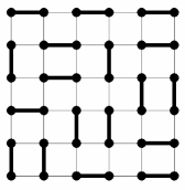
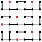
Figure 1: (Color online) Typical dimer configuration for a square lattice of size $6\times 6$ without monomer (left) and with six monomers (right, red dots).

For the general dimer problem where an arbitrary number of monomers are present – the lattice sites that are not covered by the dimers are regarded as occupied by monomers – there is no exact solution except in ${\rm 1D}$ where the solution can be expressed in terms of Chebyshev polynomials Alberici (2012), on the complete graph and on locally tree-like graphs Alberici and Contucci (2013). We can also mention that the matrix transfer method was used to express the general monomer-dimer problem Lieb (1967) (monomer density is not fixed), here the partition function, in terms of the maximum eigenvalue instead of a pfaffian. In particular a very efficient method based on variational corner transfer matrix has been found by Baxter Baxter (1968), leading to a precise approximation of thermodynamic quantities, such as the average dimer density which can be evaluated accurately as function of the dimer activity. For ${\rm 3D}$ lattices, no exact solution exists for the pure close-packed dimer problem. Recent advances concern the analytic solution of the problem where there is a single monomer on the boundary of a ${\rm 2D}$ lattice Tzeng and Wu (2003); Wu (2006), correlation functions for monomers located on the boundary Izmailian et al. (2005); Priezzhev and Ruelle (2008) and localization phenomena of a monomer in the bulk Bouttier et al. (2007); Poghosyan et al. (2011).

The field of analytical solutions in the monomer-dimer model is still uncharted, but many rigorous results exist, e.g. location of the zeros of the partition function Heilmann and Lieb (1970, 1972), series expansions of the partition function Nagle (1966) and exact recursion relation Ahrens (1981). This lack of exact solution has been formalized in the context of computer science Jerrum (1987). The importance of the dimer model in theoretical physics and combinatorics also comes from the direct mapping between the square lattice Ising model without magnetic field and the dimer model on a decorated lattice McCoy and Wu (1973); Kasteleyn (1961); Fisher (1961); Temperley and Fisher (1961) and oppositely from the mapping of the square lattice dimer model to a eight-vertex model Baxter (1972); Wu (1971) . Furthermore the Ising model in a magnetic field can be mapped to the general monomer-dimer model Heilmann and Lieb (1972).

Here we present a Grassmannian or fermionic formulation of the monomer-dimer model, which possesses an exact solution in terms of the product of two explicit pfaffians. We study the close-packed model, where an allowed dimer configuration has the property that each site of the lattice is paired with exactly one of its nearest neighbors, creating a dimer. In the simplest form, the number of dimers is the same in all the configurations, and the partition function is given by the equally-weighted average over all possible dimer configurations. In the following, we will include unequal fugacities, so that the average to be taken then includes nontrivial weighting factors.

A early representation of the dimer model was introduced using Grassmann techniques Samuel (1980a, b). A pair of these variables is attached to each site, preventing double occupancy of a site by two dimers. This leads to a direct representation of the partition function in terms of a fermionic integral over a quartic action, from which diagrammatic expansions can be carried out. We first review a very simple noncombinatorial interpretation of the ${\rm 2D}$ dimer model based on the integration over Grassmann variables Berezin (1966); Samuel (1980a, c), and factorization principles for the density matrix Hayn and Plechko (1994, 1998). A dimer model can be described with Boltzmann weights $t_{x}$ and $t_{y}$ of some coupling energy along the two directions. For example a magnetic field along one direction implies nonidentical weight values. The partition function for a lattice of size $(L\times L)$ with $L$ even can directly be written as

$$\mathcal{Q}_{0}=\int\prod_{m,n}{\rm d}\eta_{mn}(1+t_{x}\eta_{mn}\eta_{m+1n})(1+t_{y}\eta_{mn}\eta_{mn+1})$$ (1)

where $\eta_{mn}$ are nilpotent and commuting variables satisfying Barbaro et al. (1997) $\eta_{mn}^{2}=0$, $\int{\rm d}\eta_{mn}\eta_{mn}=1$, and $\int{\rm d}\eta_{mn}=0$. The integrals can be performed if we introduce, following closely Hayn and PlechkoHayn and Plechko (1994), a set of Grassmann variables $\{a_{mn},\bar{a}_{mn},b_{mn},\bar{b}_{mn}\}$ such that

$$1+t_{x}\eta_{mn}\eta_{m+1n}=$$

$$\int{\rm d}\bar{a}_{mn}{\rm d}a_{mn}e^{a_{mn}\bar{a}_{mn}}(1+a_{mn}\eta_{mn})(1+t_{x}\bar{a}_{mn}\eta_{m+1n}),$$

$$1+t_{y}\eta_{mn}\eta_{mn+1}=$$ (2)

$$\int{\rm d}\bar{b}_{mn}{\rm d}b_{mn}e^{b_{mn}\bar{b}_{mn}}(1+b_{mn}\eta_{mn})(1+t_{y}\bar{b}_{mn}\eta_{mn+1}).$$

This decomposition allows for an integration over the Grassmann variables $\eta_{mn}$, after rearranging the different link variables $A_{mn}=1+a_{mn}\eta_{mn}$, $\bar{A}_{m+1n}=1+t_{x}\bar{a}_{mn}\eta_{m+1n}$, $B_{mn}=1+b_{mn}\eta_{mn}$ and $\bar{B}_{mn+1}=1+t_{y}\bar{b}_{mn}\eta_{mn+1}$. Then the partition function becomes

$$\mathcal{Q}_{0}=\mathrm{Tr}_{\{a,\bar{a},b,\bar{b},\eta\}}\prod_{m,n}(A_{mn}\bar{A}_{m+1n})(B_{mn}\bar{B}_{mn+1}),$$ (3)

where we use the integration measure $\mathrm{Tr}_{\{.\}}$ for the different Grassmannian and nilpotent variables with the adequate weights.

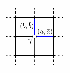
Figure 2: (Color online) Variable configuration on site and links. At each site is associated a nilpotent variable $\eta$ such that $\eta^{2}=0$, and two pairs of Grassmann variables $(a,\bar{a})$ and $(b,\bar{b})$, one for each of the two directions.

The non-commuting link variables are then moved through the product in such a way that each $\eta_{mn}$ is isolated and can be integrated directly. This rearrangement is possible in two dimensions thanks to the mirror symmetry introduced by Plechko Plechko (1985) for the ${\rm 2D}$ Ising model. This also imposes the conditions $\bar{A}_{1n}=1$, $\bar{A}_{L+1n}=1$, $\bar{B}_{m1}=1$, and $\bar{B}_{mL+1}=1$, or $\bar{a}_{0n}=\bar{a}_{Ln}=\bar{b}_{m0}=\bar{b}_{mL}=0$ for open boundary conditions. One finally obtains the following exact expression

$$\mathcal{Q}_{0}=\mathrm{Tr}_{\{a,\bar{a},b,\bar{b},\eta\}}\overrightarrow{\prod_{n}}\Big{(}\overleftarrow{\prod_{m}}\bar{B}_{mn}\overrightarrow{\prod_{m}}\bar{A}_{mn}B_{mn}A_{mn}\Big{)}.$$ (4)

The integration over the $\eta_{mn}$ variables is performed recursively from $m=1$ to $m=L$ for each $n$. Each integration leads to a Grassmann quantity $L_{mn}=a_{mn}+b_{mn}+t_{x}\bar{a}_{m-1n}+(-1)^{m+1}t_{y}\bar{b}_{mn-1}$, which is moved to the left of the products over $m$ in Eq. (4), hence a minus sign is needed in front of each $\bar{b}$ crossed by $L_{mn}$ that is moved through the product of the $\bar{B}$ terms. Finally, the result $\mathcal{Q}_{0}=\mathrm{Tr}_{\{a,\bar{a},b,\bar{b}\}}\prod_{m,n}L_{mn}$ can be further rewritten by introducing additional Grassmann variables $c_{mn}$ such that $L_{mn}=\int{\rm d}c_{mn}\exp(c_{mn}L_{mn})$. This expresses $\mathcal{Q}_{0}$ as a Gaussian integral over variables $\{a,\bar{a},b,\bar{b},c\}$. The integration over variables $\{a,\bar{a},b,\bar{b}\}$ can then be performed and, after anti-symmetrization of the expression, one obtains explicitly

$${\mathcal{Q}}_{0}=\int\prod_{m,n}{\rm d}c_{mn}\exp\sum_{m,n}\left[\frac{1}{2}t_{x}(c_{m+1n}c_{mn}-c_{m-1n}c_{mn})+\frac{1}{2}t_{y}(-1)^{m+1}(c_{mn+1}c_{mn}-c_{mn-1}c_{mn})\right]=\int\prod_{m,n}{\rm d}c_{mn}\exp{\mathcal{S}_{0}}.$$ (5)

Boundary conditions are now $c_{0,n}=c_{m,0}=c_{L+1,n}=c_{m,L+1}=0$. We consider a Fourier transformation satisfying open boundary conditions Hayn and Plechko (1994), $c_{mn}=i^{m+n}\sum_{p,q=1}^{L}c_{pq}f_{m}(p)f_{n}(q)$, where $f_{n}(p)=\sqrt{\frac{2}{L+1}}\sin\frac{\pi pn}{L+1}$ form an orthonormal set of functions $\sum_{m}f_{m}(p)f_{m}(q)=\delta_{pq}$. This leads to a block representation of the action in the momentum space, for momenta inside the reduced sector $1\leq p,q\leq L/2$. We note vectors ${\bf c}_{\alpha}=^{t}(c_{pq},c_{-pq},c_{p-q},c_{-p-q})$, where $-p$ is meant for $L+1-p$ and label $\alpha=\{p,q\}$. The four components of these vectors will be written $c_{\alpha}^{\mu}$ with $\mu=1\cdots 4$. Then $\mathcal{S}_{0}=\frac{i}{2}c_{\alpha}^{\mu}M_{\alpha}^{\mu\nu}c_{\alpha}^{\nu}$, where the antisymmetric matrix $M$ is defined by

$$M_{\alpha}=\begin{pmatrix}0&0&-a_{y}(q)&-a_{x}(p)\\ 0&0&a_{x}(p)&-a_{y}(q)\\ a_{y}(q)&-a_{x}(p)&0&0\\ a_{x}(p)&a_{y}(q)&0&0\\ \end{pmatrix}$$

with $a_{x}(p)=2t_{x}\cos\frac{\pi p}{L+1}$ and $a_{y}(q)=2t_{y}\cos\frac{\pi q}{L+1}$. The factor $i$ can be absorbed in a redefinition of the $c$’s variables. One simply obtains a product of cosine functions Hayn and Plechko (1994) as found by Kasteleyn, Temperley, and Fischer Kasteleyn (1961); Fisher (1961); Temperley and Fisher (1961), since the pfaffian of $\prod_{\alpha}M_{\alpha}$ is the product $\prod_{p,q}[a_{x}(p)^{2}+a_{y}(q)^{2}]$ in the reduced sector of momenta, or

$$\mathcal{Q}_{0}=\prod_{p,q=1}^{L/2}\left[4t_{x}^{2}\cos^{2}\frac{\pi p}{L+1}+4t_{y}^{2}\cos^{2}\frac{\pi q}{L+1}\right].$$ (6)

The matrix $M_{\alpha}$ is deeply related to the Kasteleyn Kasteleyn (1961) orientation matrix $K$ since $\mathcal{Q}_{0}={\rm Pf}(\prod_{\alpha}M_{\alpha})={\rm Pf}(K)$.

We consider now the case where an even number $n$ of monomers are present in the lattice at different fixed positions ${\bf r}_{i}=(m_{i},n_{i})$ with $i=1,\cdots,n$, see Fig. 1. The partition function $\mathcal{Q}_{n}(\{{\bf r}_{i}\})$, which we define as a correlation function between monomers after summing up over all dimer configurations, is the number of all possible dimer configurations with the constraint imposed by fixing the given monomer positions. This quantity is evaluated by inserting $\eta_{m_{i}n_{i}}$ in Eq. (1) at each monomer location, which prevents dimers from occupying these sites. It is useful to introduce additional Grassmann variables $h_{i}$ such that $\eta_{m_{i}n_{i}}=\int{\rm d}h_{i}\exp(h_{i}\eta_{m_{i}n_{i}})$. These insertions are performed at point ${\bf r}_{i}$ in Eq. (4), and the integration over $\eta_{m_{i}n_{i}}$ modifies $L_{m_{i}n_{i}}\rightarrow L_{m_{i}n_{i}}+h_{i}$. However, by moving the anticommuting variables ${\rm d}h_{i}$ to the left of the remaining ordered product, a minus sign is introduced in front of each $\bar{b}_{mn_{i}-1}$ or $t_{y}$ coupling in $\bar{B}_{mn_{i}}$ for all $m>m_{i}$. We can replace more generally $\bar{b}_{mn-1}$ by $\epsilon_{mn}\bar{b}_{mn-1}$, such that $\epsilon_{mn_{i}}=-1$ for $m>m_{i}$, and $\epsilon_{mn}=1$ otherwise. The integration is then performed on the remaining $\{a,\bar{a},b,\bar{b}\}$ variables as usual, so that $\mathcal{Q}_{n}(\{{\bf r}_{i}\})$ can be expressed as a Gaussian form, with a sum of counter-terms corresponding to the monomer insertions, or

$$\mathcal{Q}_{n}(\{{\bf r}_{i}\})=\mathrm{Tr}_{\{c,h\}}{\rm e}^{\mathcal{S}_{0}+\sum_{\{{\bf r}_{i}\}}c_{m_{i}n_{i}}h_{i}+\mathcal{S}_{I}},$$

$$\mathcal{S}_{I}=2t_{y}\sum_{\{{\bf r}_{i}\}}\sum_{m=m_{i}+1}^{L}(-1)^{m+1}c_{mn_{i}-1}c_{mn_{i}}.$$ (7)

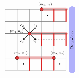
Figure 3: (Color online) Typical configuration of the system with four monomers. The sign of the couplings $t_{y}$ are reversed (red links) along the black-dashed line (or disorder operator, see text) that arises from moving the Grassmann fields conjugated to the defects toward the right boundary. Elementary vectors ${\bf{e}}_{i=1\cdots 4}$ are represented, and $\bf{e}_{4}$ indicates the starting location of the line of defects for the disorder operator.

The contribution $\mathcal{S}_{I}$ corresponds to a line of defects, as shown in Fig. 3. The addition of monomers is therefore equivalent to inserting a magnetic field $h_{i}$ at points ${\bf r}_{i}$, as well as a line of defect $c_{mn_{i}-1}c_{mn_{i}}$ running from the monomer position to the right boundary $m=L$. If two monomers have the same ordinate $n_{i}=n_{j}$, the line of defects will only run between the two mononers and will not reach the boundary. This can be viewed as an operator acting on the links crossed by the line and running from a point on the dual lattice to the boundary on the right-hand side. More specifically, we can express the correlation functions, after integration over the fermionic magnetic fields $h_{i}$, as an average over composite fields

$$\frac{\mathcal{Q}_{n}(\{{\bf r}_{i}\})}{\mathcal{Q}_{0}}=\Big{\langle}\prod_{\{{\bf r}_{i}\}}c_{m_{i}n_{i}}\exp\Big{(}2t_{y}\sum_{m=m_{i}+1}^{L}(-1)^{m+1}c_{mn_{i-1}}c_{mn_{i}}\Big{)}\Big{\rangle}_{0}=\Big{\langle}\prod_{\{{\bf r}_{i}\}}c_{m_{i}n_{i}}\mu({\bf r}_{i}+{\bf e_{4}})\Big{\rangle}_{0}=\Big{\langle}\prod_{\{{\bf r}_{i}\}}\Psi_{4}({\bf r}_{i})\Big{\rangle}_{0},$$ (8)

where $\mu({\bf r}+\bf{e}_{i})$ is a disorder operator whose role is to change the sign of the vertical links across its path starting from vector ${\bf r}+\bf{e}_{i}$ on the dual lattice toward the right hand side, see Fig. 3. The integration $\langle\cdots\rangle_{0}$ is performed relatively to the action $\mathcal{S}_{0}$. Elementary vectors $\bf{e}_{i}$ define a four-component fermionic field $\Psi_{\mu}({\bf r})=c_{mn}\mu({\bf r}+{\bf e}_{\mu})$, which is the fermionic counterpart of the scalar field introduced for the Ising-spin model Kadanoff and Ceva (1971); Polyakov (1987). In the latter case, a linear differential equation can be simply found for $\Psi_{\mu}({\bf r})=\sigma({\bf r})\mu({\bf r}+{\bf e}_{\mu})$, with $\sigma({\bf r})=\pm 1$, leading to a Dirac equation. Here the general correlator between monomers is directly mapped onto the correlator between these fermionic composite fields. If we go back to Eq. (7), the part of the field interaction can be Fourier transformed such that $\sum_{\{{\bf r}_{i}\}}c_{m_{i}n_{i}}h_{i}=\sum_{p,q=1}^{L}c_{pq}H_{pq}=\sum_{\alpha,\mu}c_{\alpha}^{\mu}H_{\alpha}^{\mu}$. The term $\mathcal{S}_{I}$ in the action can be written as $\frac{i}{2}c_{\alpha}^{\mu}V_{\alpha\beta}^{\mu\nu}c_{\beta}^{\nu}$, with the perturbative matrix $V_{\alpha\beta}$ given by

$$V_{\alpha,\beta}=V_{pq,p^{\prime}q^{\prime}}=\sum_{\{{\bf r}_{i}\}}2t_{y}(-1)^{n_{i}}\left\{\sum_{m=m_{i}+1}^{L}f_{m}(p)f_{m}(p^{\prime})\right\}\Big{(}f_{n_{i}-1}(q)f_{n_{i}}(q^{\prime})-f_{n_{i}-1}(q^{\prime})f_{n_{i}}(q)\Big{)}.$$ (9)

The different components $V_{\alpha\beta}^{\mu\nu}$ are given explicitly, for the first terms, by $V_{\alpha\beta}^{11}=V_{pq,p^{\prime}q^{\prime}}$, $V_{\alpha\beta}^{12}=V_{pq,-p^{\prime}q^{\prime}}$, $V_{\alpha\beta}^{21}=V_{-pq,p^{\prime}q^{\prime}}$, and so on. Then the full fermionic action is $\mathcal{S}=\frac{i}{2}c_{\alpha}^{\mu}W_{\alpha}^{\mu\nu}c_{\alpha}^{\nu}+c_{\alpha}^{\mu}H_{\alpha}^{\mu}$ with antisymmetric matrix $W_{\alpha\beta}^{\mu\nu}=\delta_{\alpha\beta}M_{\alpha}^{\mu\nu}+V_{\alpha\beta}^{\mu\nu}$ satisfying $W_{\alpha\beta}^{\mu\nu}=-W_{\beta\alpha}^{\nu\mu}$. By construction, this matrix can be represented as a block matrix of global size $(L^{2}\times L^{2})$

$$W=\begin{pmatrix}M_{\alpha=(1,1)}&V_{(1,1),(1,2)}&V_{(1,1),(1,3)}&\cdots&\\ -V_{(1,1),(1,2)}&M_{(1,2)}&V_{(1,2),(1,3)}&\cdots\\ -V_{(1,1),(1,3)}&-V_{(1,2),(1,3)}&M_{(1,3)}&\cdots\\ \cdots&&&\\ \lx@intercol\hfil$\upbracefill$\hfil\lx@intercol\\ \lx@intercol\hfil\scriptstyle L^{2}/4\;{\rm blocks}\hfil\lx@intercol\\ \vspace{-\normalbaselineskip}\cr\end{pmatrix},\vspace{\normalbaselineskip}$$

where each of the $(L^{2}/4)\times(L^{2}/4)$ blocks is a $(4\times 4)$ matrix. Labels $\alpha$ are ordered with increasing momentum $(1,1),(1,2)\cdots(1,L/2),(2,1)\cdots$. Then $\mathcal{Q}_{n}(\{{\bf r}_{i}\})$ can formally be written as $\mathcal{Q}_{n}(\{{\bf r}_{i}\})=\mathrm{Tr}_{\{c,h\}}\exp\left(\frac{i}{2}c_{\alpha}^{\mu}W_{\alpha\beta}^{\mu\nu}c_{\beta}^{\nu}+c_{\alpha}^{\mu}H_{\alpha}^{\mu}\right)$. The linear terms in $c_{\alpha}^{\mu}$ can be removed using a translation $c_{\alpha}^{\mu}\rightarrow c_{\alpha}^{\mu}+g_{\alpha}^{\mu}$, with $g_{\alpha}^{\mu}=i(W^{-1})_{\alpha\beta}^{\mu\nu}H_{\beta}^{\nu}$. After a further rescaling of variables $c_{\alpha}\rightarrow i^{-1/2}c_{\alpha}$, one obtains

$$\mathcal{Q}_{n}(\{{\bf r}_{i}\})={\rm Pf}(W)\mathrm{Tr}_{\{h\}}\exp\left[-\frac{i}{2}(W^{-1})_{\alpha\beta}^{\mu\nu}H_{\alpha}^{\mu}H_{\beta}^{\nu}\right].$$

The fields $H_{\alpha}^{\mu}$ depend on $h_{i}$ through the identity $H_{\alpha}^{\mu}=\sum_{i=1}^{n}\Lambda_{i,\alpha}^{\mu}h_{i}$, where coefficients $\Lambda_{i,\alpha}^{\mu}$ are expressed using a four-dimensional vector ${\bf\Lambda}_{i,\alpha}=f_{m_{i}}(p)f_{n_{i}}(q){\bf\Lambda}_{i}$. The components of momentum-independent vector $\Lambda_{i}^{\mu}$ are $(i^{m_{i}+n_{i}},-i^{-m_{i}+n_{i}},-i^{m_{i}-n_{i}},i^{-m_{i}-n_{i}})$. Its role is to fix whether the configuration of the monomers is allowed or not (in this case the correlator is zero). The final and compact expression for $\mathcal{Q}_{n}(\{{\bf r}_{i}\})$ is then

$$\mathcal{Q}_{n}(\{{\bf r}_{i}\})={\rm Pf}(W){\rm Pf}(C),$$ (10)

where $C$ is a real $(n\times n)$ antisymmetric matrix with elements $C_{ij}=-i\Lambda_{i,\alpha}^{\mu}(W^{-1})_{\alpha\beta}^{\mu\nu}\Lambda_{j,\beta}^{\nu}$. The antisymmetry can be easily verified using the antisymmetry property of $W$ or $W^{-1}$.

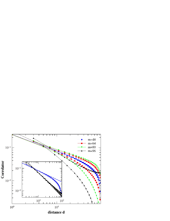
Figure 4: (Color online) Correlation function $\mathcal{Q}_{2}(\{{\bf r}_{1},{\bf r}_{2}\})\mathcal{Q}_{0}^{-1}$ for two monomers on a lattice of size $L=96$ as function of their distance $d=|{\bf r}_{2}-{\bf r}_{1}|$. They are positioned vertically, at locations ${\bf r}_{1}=(m,L/2-k)$ and ${\bf r}_{2}=(m,L/2+k+1)$, with $d=2k+1$. The curves represent different abscissa $m$ successively from the right border ($m=L=96$) to the center of the lattice ($m=48$). Curves come by pair, with lower or higher correlations, depending if $k$ is even or odd. Inset: Correlation function using Eq. (12) for two monomers on the boundary (black square symbols), at locations $n_{1}=L/2-k$ and $n_{2}=L/2+k+1$, as function of their distance $d=2k+1$. Lattice size is $L=1000$. Asymptotic limit $\frac{2}{\pi}d^{-1}$ (black dashed line) is shown for comparison. The bulk correlator (blue symbols $L=96$ and $m=48$) is also displayed, as well as its asymptotic limit $Bd^{-1/2}$ (blue dashed line). The value $B\simeq 0.247$, see text.

$\mathcal{Q}_{n}$ is therefore a product of two pfaffians where the positions of the monomers are specified in both matrices $W$ and $C$. The factorization Eq. (10) can generally be viewed as the product of a bulk and, by analogy, a boundary contribution. This can be found, for example, when a non-homogeneous magnetic field is applied at the surface of a 2D Ising model Clusel and Fortin (2006), by using Grassmann techniques as well. Here the term ${\rm Pf}(C)$ is due to the contribution of monomers in the bulk leading to a corrective factor in the free energy of order of the number $n$ of monomers, similar to a surface perturbation. Since the monomers are in the bulk, they contribute as well to the term ${\rm Pf}(W)$, which would otherwise, were the monomers located on the surface, be equal to $\mathcal{Q}_{0}$. It is worth noting that a similar factorization was found for the correlation function between two monomers in terms of the product of two spin-spin correlation functions of the Ising model at criticality Hartwig (1966); Au-Yang and Perk (1984), due to the analogy of the dimer model with two Ising models (or a complex fermionic field theory), see Appendix for precise details. It is, however, not obvious here to have such a direct identification with this result since the two pfaffians in Eq. (10) are of different nature. We can also mention that factorization of the correlation function exists in other models such as the one-dimensional XY chain Perk and Capel (1977). Matrix $V$ can be rewritten using additional matrices after considering the different components $(\mu,\nu)$. We can indeed express $V$ using four functions $u_{k}^{s=0,1}(\alpha,\beta)$, and $v_{k}^{s=0,1}(\alpha,\beta)$, for each monomer at location ${\bf r}_{k}=(m_{k},n_{k})$, with $m_{k}<L$, and such that $V_{\alpha\beta}=-2t_{y}\sum_{{\bf r}_{k}}\sum_{s,s^{\prime}=0,1}u_{k}^{s}(\alpha,\beta)\Gamma_{ss^{\prime}}v_{k}^{s^{\prime}}(\alpha,\beta)$, with

$$\Gamma_{01} = \begin{pmatrix}1&0&0&0\\ 0&1&0&0\\ 0&0&-1&0\\ 0&0&0&-1\\ \end{pmatrix},\Gamma_{11}=\begin{pmatrix}0&1&0&0\\ 1&0&0&0\\ 0&0&0&-1\\ 0&0&-1&0\\ \end{pmatrix},$$

$$\Gamma_{00} = \begin{pmatrix}0&0&1&0\\ 0&0&0&1\\ -1&0&0&0\\ 0&-1&0&0\\ \end{pmatrix},\Gamma_{10}=\begin{pmatrix}0&0&0&1\\ 0&0&1&0\\ 0&-1&0&0\\ -1&0&0&0\\ \end{pmatrix}.$$

Functions $u$ and $v$ are specified by

$$u_{k}^{s}(\alpha,\beta)=\sum_{m=m_{k}+1}^{L}(-1)^{s(m+1)}f_{m}(p)f_{m}(p^{\prime}),$$ (11)

$$\frac{v_{k}^{s}(\alpha,\beta)}{(-1)^{sn_{k}}}=\big{[}f_{n_{k}}(q)f_{n_{k}-1}(q^{\prime})+(-1)^{s}f_{n_{k}}(q^{\prime})f_{n_{k}-1}(q)\big{]}.$$

It is also worth noting that we have a similar structure in the real space, where the total action Eq. (7) is expressed by $\mathcal{S}=\frac{1}{2}c_{mn}W_{mn,m^{\prime}n^{\prime}}c_{m^{\prime}n^{\prime}}+\sum_{{\bf r}_{i}}c_{m_{i}n_{i}}h_{i}$, with $W$ containing both the connectivity matrix $M$ and the contribution of the line of defects $V$. A direct computation also leads to the factorization $\mathcal{Q}_{n}(\{{\bf r}_{i}\})={\rm Pf}(W){\rm Pf}(C)$, where $C_{ij}=(W^{-1})_{m_{i}n_{i},m_{j}n_{j}}$ is a $(n\times n)$ antisymmetric matrix.

Exact dimers enumeration algorithms Krauth (2006) up to size of $10\times 10$ has been widely used to compare with the theoretical prediction. For instance there are 636,072 different configurations of dimers with two monomers at coordinates ${\bf r}_{1}=(2,3)$ and ${\bf r}_{2}=(7,5)$ on a $8\times 8$ lattice, in accordance with the computation of $\mathcal{Q}_{2}({\bf r}_{1},{\bf r}_{2})$ taking $t_{x}=t_{y}=1$. As possible other application, we could obtain the full partition function of the monomer-dimer model by summing up over all the possible number of monomers and over all the possible positions. The result for the $8\times 8$ lattice is 179,788,343,101,980,135 Ahrens (1981), compared with the 12,988,816 configurations without monomer. In Fig. 4, we have solved numerically for a size $L=96$ the modified correlation function $\mathcal{Q}_{2}(\{{\bf r}_{1},{\bf r}_{2}\})\mathcal{Q}_{0}^{-1}={\rm Pf}(M^{-1}W){\rm Pf}(C)$, for two monomers at positions ${\bf r}_{1}=(m,L/2-k)$ and ${\bf r}_{2}=(m,L/2+k+1)$, $k=0\cdots L/2$, distant of $d=2k+1$. Due to finite-size effects, a curve for a given $m$ is distinguished depending on the parity of $k$. In the large size limit, this difference is indiscernible. Fig. 4 shows the crossover between a behavior in $d^{-1}$ near the boundary ($m=96$) to a bulk behavior Fisher and Stephenson (1963) in $d^{-1/2}$ ($m=48$). The amplitude $B$ of the asymptotic two-point correlation function, which behaves like $Bd^{-1/2}$, has been determined explicitly in the thermodynamic limit Au-Yang and Perk (1984), $B=2^{-3/4}A^{2}\approx 0.247$ with $A=2^{1/12}{\rm e}^{3\zeta^{\prime}(-1)}$ and where $\zeta(s)$ is the Riemann zeta function. This value appears to be in good agreement with our numerical fit (see inset Fig. 4, dashed blue line). Interestingly, when the monomers are located exactly on the boundary ($m=L$), $V=0$, and $W=M$, in this case $\mathcal{Q}_{n}(\{{\bf r}_{i}\})=\mathcal{Q}_{0}{\rm Pf}(C)$, and it is straightforward to compute exactly the elements of matrix $C$. In the discrete case one obtains

$$C_{ij}=\frac{4\left[(-1)^{n_{i}}-(-1)^{n_{j}}\right]}{(L+1)^{2}}\sum_{p,q=1}^{L/2}\frac{i^{1+n_{i}+n_{j}}t_{y}\cos\frac{\pi q}{L+1}\sin^{2}\frac{\pi p}{L+1}}{t_{x}^{2}\cos^{2}\frac{\pi p}{L+1}+t_{y}^{2}\cos^{2}\frac{\pi q}{L+1}}\sin\frac{\pi qn_{i}}{L+1}\sin\frac{\pi qn_{j}}{L+1}.$$ (12)

$C_{ij}$ are zero if $n_{i}$ and $n_{j}>n_{i}$ have the same parity. For example, fixing one monomer on the first site $n_{1}=1$ and taking $n_{2}=2k$, we have, for $t_{x}=t_{y}=1$ in the asymptotic limit $L\rightarrow\infty$ and large $k$, the following expansion $C_{12}\simeq\frac{2}{\pi}k^{-1}-\frac{3}{2\pi}k^{-5}$. In the case $n_{1}=L/2-k$ and $n_{2}=L/2+k+1$, as shown in inset of Fig. 4, $C_{12}\simeq\frac{2}{\pi}d^{-1}-\frac{2}{\pi}d^{-3}$ instead, with $d=2k+1$ and amplitude $2/\pi$. This result is in agreement with the work of Priezzhev and Ruelle Priezzhev and Ruelle (2008) on the scaling limit of the correlation functions of boundary monomers in a system of closely packed dimers in terms of a ${\rm 1D}$ chiral free fermion theory .

In summary, we presented a practical fermionic solution of the ${\rm 2D}$ monomer-dimer model on the square lattice, which allows for expressing the correlation functions between monomers in terms of two pfaffians, and gave an explicit formula for boundary correlations. This can also be used for studying more general $n$-point correlation functions, thermodynamical quantities, or transport phenomena of monomers. Other lattice types, such as hexagonal and other boundary conditions, can be considered as well.

We are grateful to J. H. H. Perk for his knowledge in this domain and comments on the manuscript. This work was partly supported by the Collège Doctoral Leipzig-Nancy-Coventry-Lviv (Statistical Physics of Complex Systems) of UFA-DFH.

*

Appendix A

In this section, we derive the continuum limit of the dimer action Eq. (5) and reformulate $\mathcal{S}_{0}$ in terms of two copies of Ising models. By an adequate change of variables Hayn and Plechko (1998) $c_{mn}\rightarrow i^{3/2+m^{2}}c_{mn}$, the action $\mathcal{S}_{0}$ can be written as a complex fermion field theory:

$$\mathcal{S}_{0}=\sum_{m,n}\left[\frac{1}{2}t_{x}(c_{m+1n}c_{mn}-c_{m-1n}c_{mn})+\frac{i}{2}t_{y}(c_{mn+1}c_{mn}-c_{mn-1}c_{mn})\right].$$

We can introduce the formal derivative using series expansions $c_{m+1n}=c_{mn}+\partial_{x}c_{mn}$ and $c_{mn+1}=c_{mn}+\partial_{y}c_{mn}$, up to first order in lattice elementary step, so that the action can be recognized as a purely kinetic form with no mass contribution:

$$\mathcal{S}_{0}=\sum_{m,n}\left[t_{x}\partial_{x}c_{mn}c_{mn}+it_{y}\partial_{y}c_{mn}c_{mn}\right].$$ (13)

It is convenient to define the following fields:

$$c_{-}(m,n) = c_{2m2n},\;c_{+}(m,n)=c_{2m2n+1},$$

$$\bar{c}_{-}(m,n) = c_{2m+12n+1},\;\bar{c}_{+}(m,n)=c_{2m+12n},$$ (14)

and express the previous action in terms of these fields only:

$$\mathcal{S}_{0} = -\sum_{m,n=1}^{L/2}\sum_{\sigma=\pm}\left[t_{x}(c_{\sigma}\partial_{x}\bar{c}_{-\sigma}+\bar{c}_{\sigma}\partial_{x}c_{-\sigma})\right.$$ (15)

$$+ \left.it_{y}(c_{\sigma}\partial_{y}c_{-\sigma}+\bar{c}_{\sigma}\partial_{y}\bar{c}_{-\sigma})\right].$$

Site variables $(m,n)$ now designate the locations of reduced cells containing four sites and take values between 0 and $L/2$. Field vectors $(c_{\sigma},\bar{c}_{\sigma})$ are composed of two independent components and describe two coupled Ising models labeled by index $\sigma=\pm$. This action can be diagonalized with a linear transformation, and new set of Grassmann variables:

$$\varphi_{-} = \frac{1}{2}\left(c_{-}+c_{+}+\bar{c}_{-}+\bar{c}_{+}\right),$$

$$\bar{\varphi}_{-} = \frac{1}{2}\left(c_{-}+c_{+}-\bar{c}_{-}-\bar{c}_{+}\right),$$

$$i\varphi_{+} = \frac{1}{2}\left(c_{-}-c_{+}+\bar{c}_{-}-\bar{c}_{+}\right),$$

$$i\bar{\varphi}_{+} = \frac{1}{2}\left(c_{-}-c_{+}-\bar{c}_{-}+\bar{c}_{+}\right).$$ (16)

We obtain finally a diagonalized form for $\mathcal{S}_{0}$, defining the complex derivative in two-dimensions, $\partial=t_{x}\partial_{x}+it_{y}\partial_{y}$ and $\bar{\partial}=t_{x}\partial_{x}-it_{y}\partial_{y}$:

$$\mathcal{S}_{0}=-\sum_{m,n=0}^{L/2}\left(\bar{\varphi}_{+}\bar{\partial}\bar{\varphi}_{+}-\varphi_{+}\partial\varphi_{+}-\bar{\varphi}_{-}\bar{\partial}\bar{\varphi}_{-}+\varphi_{-}\partial\varphi_{-}\right).$$

Following Plechko Plechko (1997), it is useful to introduce Dirac matrices

$$\sigma_{1}=\begin{pmatrix}0&1\\ 1&0\\ \end{pmatrix},\sigma_{2}=\begin{pmatrix}0&-i\\ i&0\\ \end{pmatrix},\sigma_{3}=\begin{pmatrix}1&0\\ 0&-1\\ \end{pmatrix},$$

and define spinor $\Psi_{\sigma}=\begin{pmatrix}\varphi_{\sigma}\\ \bar{\varphi}_{\sigma}\end{pmatrix}$. It has to be noted that $\varphi_{\sigma}$ and $\bar{\varphi}_{\sigma}$ are not conjugated but independent Grassmann variables. The action can then be put into a compact expression,

$$\mathcal{S}_{0}=\sum_{m,n=0}^{L/2}\sum_{\sigma=\pm} {}^{t}\bar{\Psi}_{\sigma}\left(\sigma_{1}\partial_{1}+\sigma_{2}\partial_{2}\right)\Psi_{\sigma},$$ (17)

where $\bar{\Psi}_{\sigma}=i\sigma_{2}\Psi_{\sigma}$ and $\partial_{1}=t_{x}\partial_{x}$, $\partial_{2}=t_{y}\partial_{y}$. Here the resulting action is of Majorana form Plechko (1997), equivalent to two independent Ising models at criticality, since no mass term is present.

References

Fowler and Rushbrooke (1937)
R. H. Fowler and
G. S. Rushbrooke,
Trans. Faraday Soc. 33,
1272 (1937).
Lovász and Plummer (1986)
L. Lovász and
M. D. Plummer,
Matching theory (Elsevier,
1986).
Flajolet and Sedgewick (2009)
P. Flajolet and
R. Sedgewick,
Analytic combinatorics (Cambridge
University Press, 2009).
Kasteleyn (1961)
P. W. Kasteleyn,
Physica 27,
1209 (1961).
Fisher (1961)
M. E. Fisher,
Phys. Rev. 124,
1664 (1961).
Temperley and Fisher (1961)
H. N. V. Temperley
and M. E.
Fisher, Philos. Mag.
6, 1061 (1961).
Fisher and Stephenson (1963)
M. E. Fisher and
J. Stephenson,
Phys. Rev. 132,
1411 (1963).
Hartwig (1966)
R. E. Hartwig,
J. Math. Phys. 7,
286 (1966).
Fisher and Hartwig (1969)
M. E. Fisher and
R. E. Hartwig, in
Stochastic Processes in Chemical Physics, edited
by K. E. Shuler
(John Wiley & Sons, 1969),
vol. 15, p. 333.
Au-Yang and Perk (1984)
H. Au-Yang and
J. H. H. Perk,
Physics Letters A 104,
131 (1984).
Kong (1987)
X. P. Kong, Ph.D. thesis,
State University of New York at Stony Brook
(1987).
Alberici (2012)
D. Alberici, Ph.D. thesis,
University of Bologna (2012).
Alberici and Contucci (2013)
D. Alberici and
P. Contucci,
arXiv preprint arXiv:1305.0838 (2013).
Lieb (1967)
E. H. Lieb, J.
Math. Phys. 8, 2339
(1967).
Baxter (1968)
R. J. Baxter,
J. Math. Phys. 9,
650 (1968).
Tzeng and Wu (2003)
W.-J. Tzeng and
F. Y. Wu, J.
Stat. Phys. 110, 671
(2003).
Wu (2006)
F. Y. Wu,
Phys. Rev. E 74,
020104(R) (2006),
erratum-ibid. 74, 039907 (2006).
Izmailian et al. (2005)
N. S. Izmailian,
V. B. Priezzhev,
P. Ruelle, and
C.-K. Hu,
Phys. Rev. Lett. 95,
260602 (2005).
Priezzhev and Ruelle (2008)
V. B. Priezzhev
and P. Ruelle,
Phys. Rev. E 77,
061126 (2008).
Bouttier et al. (2007)
J. Bouttier,
M. Bowick,
E. Guitter, and
M. Jeng,
Phys. Rev. E 76,
041140 (2007).
Poghosyan et al. (2011)
V. S. Poghosyan,
V. B. Priezzhev,
and P. Ruelle,
J. Stat. Mech.: Theory and Experiment
2011, P10004
(2011).
Heilmann and Lieb (1970)
O. J. Heilmann and
E. H. Lieb,
Phys. Rev. Lett. 24,
1412 (1970).
Heilmann and Lieb (1972)
O. J. Heilmann and
E. H. Lieb,
Commun. Math. Phys. 25,
190 (1972), reprinted in:
Statistical Mechanics, edited by B. Nachtergaele, J. P. Solovej, and J.
Yngvason, Springer (2004), pp. 45-87.
Nagle (1966)
J. F. Nagle,
Phys. Rev. 152,
190 (1966).
Ahrens (1981)
J. H. Ahrens,
Journal of Combinatorial Theory, Series A
31, 277 (1981).
Jerrum (1987)
M. R. Jerrum,
J. Stat. Phys. 48,
121 (1987), erratum-ibid 59, 1087-1088 (1990).
McCoy and Wu (1973)
B. M. McCoy and
T. T. Wu,
The Two-Dimensional Ising Model
(Harvard University Press, 1973).
Baxter (1972)
R. J. Baxter,
Ann. Phys. 70,
193 (1972).
Wu (1971)
F. W. Wu,
Phys. Rev. B 4,
2312 (1971).
Samuel (1980a)
S. Samuel, J.
Math. Phys. 21, 2806
(1980a).
Samuel (1980b)
S. Samuel, J.
Math. Phys. 21, 2820
(1980b).
Berezin (1966)
F. A. Berezin,
The Method of second quantization
(Academic Press, 1966).
Samuel (1980c)
S. Samuel, J.
Math. Phys. 21, 2815
(1980c).
Hayn and Plechko (1994)
R. Hayn and
V. N. Plechko,
J. Phys. A: Mathematical and General
27, 4753 (1994).
Hayn and Plechko (1998)
R. Hayn and
V. N. Plechko,
Physics of Atomic Nuclei 61,
1972 (1998).
Barbaro et al. (1997)
M. B. Barbaro,
A. Molinari, and
F. Palumbo,
Nucl. Phys. B 487,
492 (1997).
Plechko (1985)
V. N. Plechko,
Theoretical and Mathematical Physics
64, 748 (1985).
Kadanoff and Ceva (1971)
L. P. Kadanoff and
H. Ceva,
Phys. Rev. B 3,
3918 (1971).
Polyakov (1987)
A. M. Polyakov,
Gauge fields and strings, vol. 3 in
Contemporary Concepts in Physics (Harwood Academic
Publishers, 1987).
Clusel and Fortin (2006)
M. Clusel and
J.-Y. Fortin,
J. Phys. A: Mathematical and General
39, 995 (2006).
Perk and Capel (1977)
J. H. H. Perk and
H. W. Capel,
Physica A: Statistical Mechanics and its Applications
89, 265 (1977).
Krauth (2006)
W. Krauth,
Volume 13 of Oxford master series in statistical,
computational, and theoretical physics (Oxford
University Press, 2006).
Plechko (1997)
V. N. Plechko,
J. Phys. Studies 1,
554 (1997).