A Generalized Robust Filtering Framework for Nonlinear Differential-Algebraic Systems

Abstract

A generalized dynamical robust nonlinear filtering framework is established for a class of Lipschitz differential algebraic systems, in which the nonlinearities appear both in the state and measured output equations. The system is assumed to be affected by norm-bounded disturbance and to have both norm-bounded uncertainties in the realization matrices as well as nonlinear model uncertainties. We synthesize a robust $H_{\infty}$ filter through semidefinite programming and strict linear matrix inequalities (LMIs). The admissible Lipschitz constants of the nonlinear functions are maximized through LMI optimization. The resulting $H_{\infty}$ filter guarantees asymptotic stability of the estimation error dynamics with prespecified disturbance attenuation level and is robust against time-varying parametric uncertainties as well as Lipschitz nonlinear additive uncertainty. Explicit bound on the tolerable nonlinear uncertainty is derived based on a norm-wise robustness analysis.

Department of Research and Development, Maplesoft, Waterloo, Ontario, Canada

keywords: Robust Filtering, Nonlinear $H_{\infty}$, Differential Algebraic Equations, Descriptor Systems, Semidefinite Programming

1 Introduction

State estimation and filtering of nonlinear dynamical systems has been a subject of extensive research in recent years due to its theoretical and practical importance. State estimators are essential for observer-based control, fault detection and isolation, prediction and smoothing, and monitoring purposes. Generalizing the state space modeling, descriptor systems can characterize a larger class of systems than conventional state space models and can describe the physics of the system more precisely. Descriptor systems, also referred to as singular systems or differential-algebraic equation (DAE) systems, arise from an inherent and natural modeling approach, and have vast applications in engineering disciplines such as power systems, network and circuit analysis, and multibody mechanical systems, as well as in social and economic sciences. Model based development (MBD) processes are adopted in advanced control methodologies in areas such as in automotive, energy, mechatronics and aerospace. Recently, DAE systems have become a fundamental part of physical modeling and simulation of dynamical system. The number of models described by DAEs has been rapidly growing, partly due to modern modeling tools, such as those based on the Modelica object oriented modeling language [16, 10].

As more and more DAE models are available, it is natural to directly use them for controller or filter design. Many approaches have been developed to design state observers for descriptor systems. In [11, 9, 18, 13, 14, 12, 33, 23, 34, 26, 31, 36, 8, 7] various methods of observer design for linear and nonlinear descriptor systems have been proposed. In [9] an observer design procedure is proposed for a class nonlinear descriptor systems using an appropriate coordinate transformation. In [31], the authors address the unknown input observer design problem dividing the system into two dynamic and static subsystems. References [12, 23] study the full order and reduced order observer design for Lipschitz nonlinear systems.

Three aspects of robust filtering approaches:

A fundamental limitation encountered in conventional observer theory is that it cannot guarantee observer performance in the presence of model uncertainties and/or disturbances and measurement noise. One of the most popular ways to deal with the nonlinear state estimation problem is the extended Kalman filtering. However, the requirements of specific noise statistics and weakly nonlinear dynamics, has restricted its applicability to nonlinear systems. To deal with the nonlinear filtering problem in the presence of model uncertainties and unknown exogenous disturbances, we can resort the robust $H_{\infty}$ or similar filtering approaches. A robust filtering approach accomplishes the following objectives:

• Stability: In the absence of external disturbances, the filter error asymptotically converges to zero. Moreover, our design is such that it can maximize the size of the Lipschitz constant that can be tolerated in the system which directly translates to the expansion of the admissible region of operation.

• Robustness: The design is robust with respect to uncertainties in the nonlinear plant model.

• Filtering: The effect of exogenous disturbances on the filter error can be minimized.

To deal with the nonlinear state observation problem in the presence of model uncertainties and unknown exogenous disturbances, the robust $H_{\infty}$ filtering was proposed as an effective approach. In $H_{\infty}$ filtering, the $\mathcal{L}_{2}$ gain from the exogenous disturbance to the filter error is guaranteed to be less than a prespecified level. Therefore, this $\mathcal{L}_{2}$ gain minimization is in fact an energy-to-energy filtering problem. The disturbance can be any signal with finite energy, either stochastic (with unknown statistics) or deterministic. See for example references [15], [35] and the references therein. In these references, the authors consider a class of continuous-time nonlinear system satisfying a Lipschitz continuity condition. The mathematical system model is assumed to be affected by time-varying parametric uncertainties and norm bounded disturbances affect the measurements. Under these conditions they obtain Riccati-based sufficient conditions for the stability of the proposed filter with guaranteed disturbance attenuation level. In the absence of disturbance, of course, the solution of the filtering problem renders an asymptotic observer whose state converges to the plant state. We point out here that the elegance of the Riccati approach comes at the price of somewhat restrictive regularity assumptions required in the solution of the synthesis problem. These restrictions are not inherent in the $H_{\infty}$ formulation but are a consequence of the Riccati approach and can be relaxed using Linear Matrix inequalities (LMIs).

In this work, we study the robust nonlinear $H_{\infty}$ filtering criterion for continuous-time Lipschitz DAE (descriptor) systems in the presence of disturbance and model uncertainties, in a linear matrix inequalities (LMI) framework. The linear matrix inequalities proposed here are developed in such a way that the admissible Lipschitz constant of the system is maximized through LMI optimization. This adds the important extra feature to the filter, making it robust against a class of nonlinear uncertainty. Securing the same filter features, the LMI optimization approach to nonlinear filtering for the conventional state space models can be found in [1, 2, 5] and [3, 4] in continuous and discrete time domains, respectively. The results given here generalize our previous results in that: i) extend the model from conventional state space to descriptor models, ii) consider nonlinearities in both the state and output equations, and iii) generalize the filter structure by proposing a general dynamical filtering framework that can easily capture both dynamic and static-gain filter structures. The proposed dynamical structure has additional degree of freedom compared to conventional static-gain filters and consequently is capable of robustly stabilizing the filter error dynamics for systems for which an static-gain filter cannot be found. Besides, for the cases that both static-gain and dynamic filters exist, the maximum admissible Lipschitz constant obtained using the proposed dynamical filter structure can be much larger than that of the static-gain filter. The result is a filter with a prespecified disturbance attenuation level which guarantees asymptotic stability of the estimation error dynamics and is robust against Lipschitz nonlinear uncertainties as well as time-varying parametric uncertainties, simultaneously.

In section II, the problem statement and some preliminaries are mentioned. In section III, we propose a new method for robust $H_{\infty}$ filter design for nonlinear descriptor uncertain systems based on semidefinite programming (SDP). In Section IV, the SDP problem of Section III is converted into strict LMIs. Section V, is devoted to robustness analysis in which an explicit bound on the tolerable nonlinear uncertainty is derived. In section VI, we show the effectiveness of our proposed filter design procedure through an illustrative example. Section VII includes our concluding remarks and some proposed future research directions.

2 Preliminaries and Problem Statement

Consider the following class of continuous-time uncertain nonlinear descriptor systems:

$$\left(\Sigma_{s}\right):\mathbf{E}\dot{x}(t) =(A+\Delta A(t))x(t)+\Phi(x,u)+Bw(t)$$ (1)

$$y(t) =(C+\Delta C(t))x(t)+\Psi(x,u)+Dw(t)$$ (2)

where $x\in{\mathbb{R}}^{n},u\in{\mathbb{R}}^{m},y\in{\mathbb{R}}^{p}$ and $\Phi(x,u)$ and $\Psi(x,u)$ contain nonlinearities of second order or higher. $\mathbf{E}$, $A$, $B$, $C$ and $D$ are constant matrices with compatible dimensions. The matrix $\mathbf{E}$, which following the analogy from the multibody dynamics modeling, is often referred to as the mass matrix, may be singular. When the matrix $\mathbf{E}$ is singular, the above form is equivalent to a set of differential-algebraic equations (DAEs) [11]. In other words, the dynamics of descriptor systems, comprise a set of differential equations together with a set of algebraic constraints. Unlike conventional state space systems in which the initial conditions can be freely chosen in the operating region, in the descriptor systems, initial conditions must be consistent, i.e. they should satisfy the algebraic constraints. Consistent initialization of descriptor systems naturally happens in physical systems but should be taken into account when simulating such systems [27]. Without loss of generality, we assume that $0<rank(\mathbf{E})=s\leq n$; $x(0)=x_{0}$ is a consistent (unknown) set of initial conditions. If the matrix $\mathbf{E}$ is non-singular (i.e. full rank), then the descriptor form reduces to the conventional state space. The number of algebraic constraints that must be satisfied by $x_{0}$ equals $n-s$. We assume the pair $(\mathbf{E},A)$ to be regular, i.e. $\det(s\mathbf{E}-A)\neq 0$ for some $s\in\mathbb{C}$ [11] and impulse free, i.e. $deg\det(s\mathbf{E}-A)=rank(\mathbf{E})$ [11], and the triple $(\mathbf{E},A,C)$ to be observable, i.e. [19]

$$rank\left[\begin{array}[]{c}s\mathbf{E}-A\\ C\\ \end{array}\right]=n,\ \forall\ s\in\mathbb{C}.$$ (5)

We also assume that the system (1)-(2) is locally Lipschitz with respect to $x$ in a region $\mathcal{D}$ containing the origin, uniformly in $u$, i.e.:

$$\Phi(0,u^{*})=\Psi(0,u^{*})=0,$$

$$\|\Phi(x_{1},u^{*})-\Phi(x_{2},u^{*})\|\leqslant\gamma_{1}\|x_{1}-x_{2}\|,\hskip 5.69054pt\forall\,x_{1},x_{2}\in\mathcal{D}$$

$$\|\Psi(x_{1},u^{*})-\Psi(x_{2},u^{*})\|\leqslant\gamma_{2}\|x_{1}-x_{2}\|,\hskip 5.69054pt\forall\,x_{1},x_{2}\in\mathcal{D}$$

where $\|.\|$ is the induced 2-norm, $u^{*}$ is any admissible control signal and $\gamma_{1},\ \gamma_{2}>0$ are the Lipschitz constants of $\Phi(x,u)$ and $\Psi(x,u)$, respectively, the $\mathcal{D}$ is the operating region. If the nonlinear functions $\Phi(x,u)$ and $\Psi(x,u)$ satisfy the Lipschitz continuity condition globally in $\mathbb{R}^{n}$, then the results will be valid globally. The Lipschitz continuity condition is not a restrictive assumption since most nonlinear function are Lipschitz continuous at least locally. Particularly, all continuously differentiable functions are known to be Lipschitz, and their Lipschitz constant is computed as the supremum of their Jacobian matrix over the operating region [25]. As a usual assumption in robust filtering techniques, we also assume that the system under consideration is stable.

$w(t)\in\mathcal{L}_{2}[0,\infty)$ is an unknown exogenous disturbance, and $\Delta A(t)$ and $\Delta C(t)$ are unknown matrices representing time-varying parameter uncertainties, and are assumed to be of the form

$$\left[\begin{array}[]{c}\Delta A(t)\\ \Delta C(t)\\ \end{array}\right]=\left[\begin{array}[]{c}M_{1}\\ M_{2}\\ \end{array}\right]F(t)N$$ (10)

where $M_{1}$, $M_{2}$ and $N$ are known real constant matrices and $F(t)$ is an unknown real-valued time-varying matrix satisfying

$$F^{T}(t)F(t)\leq I\hskip 28.45274pt\forall\ t\in[0,\infty).$$ (11)

The parameter uncertainty in the linear terms can be regarded as the variation of the operating point of the nonlinear system. It is also worth noting that the structure of parameter uncertainties in (10) has been widely used in the problems of robust control and robust filtering for both continuous-time and discrete-time systems and can capture the uncertainty in a number of practical situations [15], [20].

2.1 Filter Structure

We propose the general filtering framework of the following form

$$\begin{split}\left(\Sigma_{o}\right):\mathbf{E}\dot{x}_{F}(t)&=A_{F}x_{F}(t)+B_{F}y(t)+\mathcal{E}_{1}\Phi(x_{F},u)\\ &\ \ \ +\mathcal{E}_{2}\Psi(x_{F},u)\\ z_{F}(t)&=C_{F}x_{F}(t)+D_{F}y(t)+\mathcal{E}_{3}\Psi(x_{F},u).\end{split}$$ (12)

The proposed framework can capture both dynamic and static-gain filter structures by proper selection of $\mathcal{E}_{1}$, $\mathcal{E}_{2}$ and $\mathcal{E}_{3}$. Choosing $\mathcal{E}_{1}=I$, $\mathcal{E}_{2}=0$ and $\mathcal{E}_{3}=0$ leads to the following dynamic filter structure:

$$\begin{split}\mathbf{E}\dot{x}_{F}(t)&=A_{F}x_{F}(t)+B_{F}y(t)+\Phi(x_{F},u)\\ z_{F}(t)&=C_{F}x_{F}(t)+D_{F}y(t).\end{split}$$ (13)

Furthermore, for the static-gain filter structure we have:

$$\begin{split}\mathbf{E}\dot{x}_{F}(t)&=Ax_{F}(t)+\Phi(x_{F},u)\\ &\ \ +L[y(t)-Cx_{F}(t)-\Psi(x_{F},u)]\\ z_{F}(t)&=x_{F}(t).\end{split}$$ (14)

Hence, with

$$A_{F} =A-LC,\ B_{F}=L,\ C_{F}=I,\ D_{F}=0,$$

$$\mathcal{E}_{1} =I,\ \mathcal{E}_{2}=-L,\ \mathcal{E}_{3}=0,$$

the general filter captures the well-known static-gain observer filter structure as a special case. We prove our result for the general filter of class $(\Sigma_{o})$.

Now, suppose that

$$z(t)=Hx(t)$$ (15)

stands for the controlled output for states to be estimated where $H$ is a known matrix. The estimation error is defined as

$$e(t)\triangleq z(t)-z_{F}(t)=-C_{F}x_{F}+(H-D_{F}C-D_{F}\Delta C)x\\ -D_{F}\Psi(x,u)-\mathcal{E}_{3}\Psi(x_{F},u)-D_{F}Dw.$$ (16)

The filter error dynamics is given by

$$\left(\Sigma_{e}\right):\mathbf{\widetilde{E}}\dot{\xi}(t) =(\widetilde{A}+\Delta\widetilde{A})\xi(t)+S_{1}\Omega(\xi,u)+\widetilde{B}w(t)$$ (17)

$$e(t) =(\widetilde{C}+\Delta\widetilde{C})\xi(t)+S_{2}\Omega(\xi,u)+\widetilde{D}w(t),$$ (18)

where,

$$\xi\triangleq\left[\begin{array}[]{c}x_{F}\\ x\\ \end{array}\right],\widetilde{A}=\left[\begin{array}[]{cc}A_{F}&B_{F}C\\ 0&A\\ \end{array}\right],\Delta\widetilde{A}=\left[\begin{array}[]{cc}0&B_{F}\Delta C\\ 0&\Delta A\\ \end{array}\right]$$ (25)

$$\mathbf{\widetilde{E}}=\left[\begin{array}[]{cc}\mathbf{E}&0\\ 0&\mathbf{E}\\ \end{array}\right],\widetilde{B}=\left[\begin{array}[]{c}B_{F}D\\ B\\ \end{array}\right],\widetilde{D}=-D_{F}D$$ (30)

$$\widetilde{C}=\left[\begin{array}[]{cc}-C_{F}&H-D_{F}C\\ \end{array}\right],\Delta\widetilde{C}=\left[\begin{array}[]{cc}0&-D_{F}\Delta C\\ \end{array}\right]$$ (33)

$$\Omega(\xi,u)=\left[\begin{array}[]{cccc}\Phi(x,u)&\Psi(x,u)&\Phi(x_{F},u)&\Psi(x_{F},u)\end{array}\right]^{T}$$ (35)

$$S_{1}=\left[\begin{array}[]{cccc}0&B_{F}&\mathcal{E}_{1}&\mathcal{E}_{2}\\ I&0&0&0\\ \end{array}\right],S_{2}=\left[\begin{array}[]{cccc}0&-D_{F}&0&-\mathcal{E}_{3}\\ \end{array}\right].$$ (39)

For the nonlinear function $\Omega$, it is easy to show that

$$\Gamma\triangleq\left[\begin{array}[]{cccc}0&0&\gamma_{1}&\gamma_{2}\\ \gamma_{1}&\gamma_{2}&0&0\\ \end{array}\right]^{T}$$ (42)

$$\|\Omega(\xi_{1},u)-\Omega(\xi_{2},u)\|\leq\|\Gamma(\xi_{1}-\xi_{2})\|\leq\|\Gamma\|\|\xi_{1}-\xi_{2}\|$$

$$\ \ =\sqrt{\gamma_{1}^{2}+\gamma_{2}^{2}}\|\xi_{1}-\xi_{2}\|\triangleq\gamma\|\xi_{1}-\xi_{2}\|.$$ (43)

Thus, the filter error system is Lipschitz with Lipschitz constant $\gamma$.

2.2 Disturbance Attenuation Level

Our purpose is to design the filter matrices $A_{F}$, $B_{F}$, $C_{F}$ and $D_{F}$ such that the filter error dynamics is asymptotically stable with maximum admissible Lipschitz constant and the following specified $H_{\infty}$ norm upper bound is simultaneously guaranteed.

$$\|e\|\leq\mu\|w\|.$$ (44)

In the following, we mention some useful lemmas that will be used later in the proof of our results.

Lemma 1. [35] For any $x,y\in\mathbb{R}^{n}$ and any positive definite matrix $P\in\mathbb{R}^{n\times{n}}$, we have

$$2x^{T}y\leq x^{T}Px+y^{T}P^{-1}y.$$

Lemma 2. [35] Let $A,D,E,F$ and P be real matrices of appropriate dimensions with $P>0$ and $F$ satisfying $F^{T}F\leq I$. Then for any scalar $\epsilon>0$ satisfying $P^{-1}-\epsilon^{-1}DD^{T}>0$, we have

$$\begin{split}(A+DFE)^{T}P(A+DFE)\leq&A^{T}(P^{-1}-\epsilon^{-1}DD^{T})^{-1}A+\epsilon E^{T}E.\end{split}$$

Lemma 3. [17, p. 301] A matrix $A\in\mathbb{R}^{n\times n}$ is invertible if there is a matrix norm $\||.\||$ such that $\||I-A\||<1$.

The symbol $\||.\||$ in the above lemma represents any matrix norm.

3 $H_{\infty}$ Filter Synthesis

In this section, an $H_{\infty}$ filter with guaranteed disturbance attenuation level $\mu$ is proposed. The admissible Lipschitz constant is maximized through LMI optimization. Theorem 1, introduces a design method for such a filter. It worths mentioning that unlike the Riccati approach of [15], in the LMI approach no $H_{\infty}$ regularity assumption is needed.

Theorem 1. Consider the Lipschitz nonlinear system $\left(\Sigma_{s}\right)$ along with the general filter $\left(\Sigma_{o}\right)$. The filter error dynamics is (globally) asymptotically stable with maximum admissible Lipschitz constant, $\gamma^{*}$, and guaranteed $\mathfrak{L}_{2}(w\rightarrow e)$ gain, $\mu$, if there exists a fixed scalar $\mu>0$, scalars $\epsilon_{1}>0$, $\epsilon_{2}>0$, $\alpha_{1}>0$ and $\alpha_{2}>0$ and matrices $C_{F}$, $D_{F}$, $P_{1}$, $P_{2}$, $G_{1}$, $G_{2}$ and $\mathcal{E}_{3}$ such that the following optimization problem has a solution.

$$\hskip 14.22636pt\min(2\alpha_{1}+\alpha_{2})$$

s.t.

$$\Xi_{1}=\left[\begin{array}[]{ccccc}\Pi_{1}&\Pi_{2}&0&\Pi_{3}&\Pi_{4}\\ \star&\Pi_{5}&\Pi_{6}&0&0\\ \star&\star&\Pi_{7}&0&0\\ \star&\star&\star&\Pi_{8}&0\\ \star&\star&\star&\star&\Pi_{9}\\ \end{array}\right]<0$$ (50)

$$\Xi_{2}=\left[\begin{array}[]{ccc}\epsilon_{2}I&0&-D_{F}M_{2}\\ \star&I&0\\ \star&\star&I\\ \end{array}\right]>0$$ (54)

$$\Xi_{3}=\left[\begin{array}[]{ccc}\alpha_{1}I&\mathcal{E}_{3}&D_{F}\\ \star&\alpha_{1}I&0\\ \star&\star&\alpha_{1}I\end{array}\right]>0$$ (58)

$$\Xi_{4}=\left[\begin{array}[]{cc}I&I-P_{1}^{T}\\ \star&I\\ \end{array}\right]>0$$ (61)

$$\mathbf{E}^{T}P_{1}=P_{1}^{T}\mathbf{E}\geq 0$$ (62)

$$\mathbf{E}^{T}P_{2}=P_{2}^{T}\mathbf{E}\geq 0$$ (63)

where the elements of $\Xi_{1}$ are as defined in the following, $\Lambda_{1}=G_{1}^{T}+G_{1}$, $\Lambda_{2}=A^{T}P_{2}+P_{2}A+(\epsilon_{1}+\epsilon_{2})N^{T}N$ and $\Lambda_{3}=H^{T}-C^{T}D_{F}^{T}$.

$$\Pi_{1}=\left[\begin{array}[]{ccc}\Lambda_{1}&G_{2}C&I\\ \star&\Lambda_{2}&0\\ \star&\star&-\alpha_{2}I\\ \end{array}\right],\Pi_{4}=\left[\begin{array}[]{cc}G_{2}D&0\\ P_{2}B&0\\ 0&0\\ \end{array}\right],$$ (70)

$$\Pi_{2}=\left[\begin{array}[]{ccc}0&G_{2}M_{2}&-C_{F}^{T}\\ 0&P_{2}M_{1}&\Lambda_{3}\\ 0&0&0\\ \end{array}\right],\Pi_{6}=\left[\begin{array}[]{cc}0&0\\ 0&0\\ 0&-D_{F}M_{2}\\ \end{array}\right],$$ (77)

$$\Pi_{3}=\left[\begin{array}[]{cccc}0&G_{2}&P_{1}\mathcal{E}_{1}&P_{1}\mathcal{E}_{2}\\ P_{2}&0&0&0\\ 0&0&0&0\\ \end{array}\right],$$ (81)

$$\Pi_{5}=diag(-\epsilon_{1}I,-\epsilon_{1}I,-\frac{1}{3}I),\Pi_{7}=diag(-\frac{1}{3}\epsilon_{2}I,-\frac{1}{3}\epsilon_{2}I),$$

$$\Pi_{8}=diag(-I,-I,-I,-I),\Pi_{9}=\left[\begin{array}[]{cc}-\mu^{2}I&-D^{T}D_{F}^{T}\\ \star&-\frac{1}{3}I\\ \end{array}\right].$$ (84)

Once the problem is solved:

$$A_{F} =P^{-1}_{1}G_{1},$$ (85)

$$B_{F} =P^{-1}_{1}G_{2},$$ (86)

$$C_{F}\ \text{and}\ D_{F}\ \text{are directly obtained},$$

$$\alpha_{1}^{*} \triangleq\min(\alpha_{1}),$$ (87)

$$\alpha_{2}^{*} \triangleq\min(\alpha_{2}),$$ (88)

$$\gamma^{*} \triangleq\max(\gamma)=\frac{1}{\sqrt{\alpha_{2}^{*}(1+3{\alpha_{1}^{*}}^{2})}}.$$ (89)

Proof: Consider the following Lyapunov function candidate

$$V(\xi(t))=\xi^{T}\mathbf{\widetilde{E}}^{T}P\xi.$$ (90)

To prove the stability of the filter error dynamics, we employ the well-established generalized Lyapunov stability theory as discussed in [34], [26] and [19] and the references therein. The generalized Lyapunov stability theory is mainly based on an extended version of the well-known LaSalle’s invariance principle for descriptor systems. Based on this theory, the above function along with the conditions (62) and (63) is a generalized Lyapunov function (GLF) for the system $\left(\Sigma_{e}\right)$ where $P=diag(P_{1},P_{2})$. In fact, it can be shown that $V(\xi(t))=0$ if and only if $\mathbf{\widetilde{E}}\xi=0$ and positive elsewhere [34, Ch. 2]. Now, we calculate the derivative of $V$ along the trajectories of $\left(\Sigma_{e}\right)$. We have

$$\begin{split}\dot{V}&=\dot{\xi}^{T}\mathbf{\widetilde{E}}^{T}P\xi+\xi^{T}\mathbf{\widetilde{E}}^{T}P\dot{\xi}=2\xi^{T}(\widetilde{A}+\Delta\widetilde{A})^{T}P\xi\\ &\ \ \ +2\xi^{T}PS_{1}\Omega+2\xi^{T}P\widetilde{B}w.\end{split}$$ (91)

Now, we define

$$J\triangleq\int^{\infty}_{0}(e^{T}e-\mu^{2}w^{T}w)dt.$$ (92)

Therefore

$$J<\int^{\infty}_{0}(e^{T}e-\mu^{2}w^{T}w+\dot{V})dt$$ (93)

so a sufficient condition for $J\leq 0$ is that

$$\forall t\in[0,\infty),\hskip 14.22636pte^{T}e-\mu^{2}w^{T}w+\dot{V}\leq 0.$$ (94)

We have

$$\begin{split}e^{T}e&=\xi^{T}(\widetilde{C}+\Delta\widetilde{C})^{T}(\widetilde{C}+\Delta\widetilde{C})\xi+2\xi^{T}(\widetilde{C}+\Delta\widetilde{C})^{T}S_{2}\Omega\\ &\ \ +2\xi^{T}(\widetilde{C}+\Delta\widetilde{C})^{T}\widetilde{D}w+2w^{T}\widetilde{D}^{T}S_{2}\Omega\\ &\ \ +\Omega^{T}S_{2}^{T}S_{2}\Omega+w^{T}\widetilde{D}^{T}\widetilde{D}w\end{split}$$

Thus, using Lemma 1,

$$\begin{split}\dot{V}&+e^{T}e-\mu^{2}w^{T}w\leq 2\xi^{T}(\widetilde{A}+\Delta\widetilde{A})^{T}P\xi+2\xi^{T}PS_{1}\Omega\\ &+2\xi^{T}P\widetilde{B}w-\mu^{2}w^{T}w+2\xi^{T}(\widetilde{C}+\Delta\widetilde{C})^{T}(\widetilde{C}+\Delta\widetilde{C})\xi\\ &+2\xi^{T}(\widetilde{C}+\Delta\widetilde{C})^{T}\widetilde{D}w+3\Omega^{T}S_{2}^{T}S_{2}\Omega+2w^{T}\widetilde{D}^{T}\widetilde{D}w\\ &\leq\xi^{T}[2(\widetilde{A}+\Delta\widetilde{A})^{T}P+PS_{1}^{T}S_{1}P+2(\widetilde{C}+\Delta\widetilde{C})^{T}\cdots\end{split}$$

$$\begin{split}&\cdots(\widetilde{C}+\Delta\widetilde{C})]\xi+\xi^{T}[2P\widetilde{B}+2(\widetilde{C}+\Delta\widetilde{C})^{T}\widetilde{D}]w\\ &+\Omega^{T}\Omega+3\Omega^{T}S_{2}^{T}S_{2}\Omega+w^{T}(2\widetilde{D}^{T}\widetilde{D}-\mu^{2}I)w\\ &\leq\xi^{T}[2(\widetilde{A}+\Delta\widetilde{A})^{T}P+PS_{1}^{T}S_{1}P+3(\widetilde{C}+\Delta\widetilde{C})^{T}\cdots\\ &\cdots(\widetilde{C}+\Delta\widetilde{C})]\xi+2\xi^{T}P\widetilde{B}w+\Omega^{T}\Omega+3\Omega^{T}S_{2}^{T}S_{2}\Omega\\ &+w^{T}(3\widetilde{D}^{T}\widetilde{D}-\mu^{2}I)w.\end{split}$$ (95)

Without loss of generality, we assume that there is a scalar $\alpha_{1}$ such that $\|\mathcal{E}_{3}\mathcal{E}_{3}^{T}+D_{F}D_{F}^{T}\|<\alpha_{1}^{2}$ where, $\alpha_{1}>0$ is an unknown variable. Thus,

$$\begin{split}\Omega^{T}\Omega&+3\Omega^{T}S_{2}^{T}S_{2}\Omega\leq(1+3\|S_{2}^{T}S_{2}\|)\Omega^{T}\Omega\\ &=(1+3\|S_{2}S_{2}^{T}\|)\Omega^{T}\Omega\\ &=[1+3\|\mathcal{E}_{3}\mathcal{E}_{3}^{T}+D_{F}D_{F}^{T}\|]\Omega^{T}\Omega\\ &<(1+3\alpha_{1}^{2})\Omega^{T}\Omega\\ &\leq(1+3\alpha_{1}^{2})\xi^{T}\Gamma^{T}\Gamma\xi\\ &\leq(1+3\alpha_{1}^{2})\gamma^{2}\xi^{T}\xi.\end{split}$$ (96)

Note that $\Omega(0,u)=0$. Now, defining the change of variables

$$\alpha_{2} \triangleq\frac{1}{(1+3\alpha_{1}^{2})\gamma^{2}}\Rightarrow\gamma=\frac{1}{\sqrt{\alpha_{2}(1+3{\alpha_{1}}^{2})}},$$ (97)

we have

$$\Omega^{T}\Omega+3\Omega^{T}S_{2}^{T}S_{2}\Omega<\alpha_{2}^{-1}\xi^{T}\xi.$$ (98)

It is worth mentioning that the change of variables in (97) plays a vital role here. The alternative changes of variables such as $\alpha_{2}=\alpha_{1}\gamma$ which may seem more straightforward, would make $\gamma$ appear in $\Xi_{1}$ and then due to the existence of $\alpha_{1}$ in the LMI (58), the variables $\alpha_{1}$ and $\gamma$ would be over-determined.
On the other hand,

$$\Delta\widetilde{A} =\left[\begin{array}[]{cc}0&B_{F}\Delta C\\ 0&\Delta A\\ \end{array}\right]=\left[\begin{array}[]{cc}0&B_{F}M_{2}FN\\ 0&M_{1}FN\\ \end{array}\right]$$ (103)

$$=\left[\begin{array}[]{cc}0&B_{F}M_{2}\\ 0&M_{1}\\ \end{array}\right]F\left[\begin{array}[]{cc}0&0\\ 0&N\\ \end{array}\right]\triangleq\widetilde{M_{1}}F\widetilde{N}$$ (108)

$$\Delta\widetilde{C} =\left[\begin{array}[]{cc}0&-D_{F}\Delta C\\ \end{array}\right]=\left[\begin{array}[]{cc}0&-D_{F}M_{2}FN\\ \end{array}\right]$$ (111)

$$=\left[\begin{array}[]{cc}0&-D_{F}M_{2}\\ \end{array}\right]F\left[\begin{array}[]{cc}0&0\\ 0&N\\ \end{array}\right]\triangleq\widetilde{M_{2}}F\widetilde{N}.$$ (115)

Therefore, based on (96) and (97) and using Lemma 2 we can write

$$\begin{split}\dot{V}&+e^{T}e-\mu^{2}w^{T}w<\xi^{T}[\widetilde{A}^{T}P+P\widetilde{A}+\epsilon_{1}\widetilde{N}^{T}N\\ &+\epsilon_{1}^{-1}P\widetilde{M}_{1}\widetilde{M}_{1}P+3\widetilde{C}^{T}(I-\epsilon_{2}^{-1}\widetilde{M}_{2}\widetilde{M}_{2}^{T})^{-1}\widetilde{C}\\ &+\epsilon_{2}\widetilde{N}^{T}N+PS_{1}S_{1}^{T}P+\alpha_{2}^{-1}]\xi+2\xi^{T}P\widetilde{B}w\\ &+w^{T}(3\widetilde{D}^{T}\widetilde{D}-\mu^{2}I)w.\end{split}$$ (116)

Now, a sufficient condition for (94) is that the right hand side of (116) be negative definite. Using Schur complements, this is equivalent to the following LMI. Note that having $w=0$, (91) is already included in (95) and consequently in (116).

$$\left[\begin{array}[]{cccccccc}\Upsilon&I&P\widetilde{M}_{1}&\widetilde{C}^{T}&0&PS_{1}&P\widetilde{B}&0\\ \star&-\alpha_{2}I&0&0&0&0&0&0\\ \star&\star&-\epsilon_{1}I&0&0&0&0&0\\ \star&\star&\star&-\frac{1}{3}I&\widetilde{M}_{2}&0&0&0\\ \star&\star&\star&\star&-\frac{\epsilon_{2}}{3}I&0&0&0\\ \star&\star&\star&\star&\star&-I&0&0\\ \star&\star&\star&\star&\star&\star&-\mu^{2}I&\widetilde{D}^{T}\\ \star&\star&\star&\star&\star&\star&\star&-\frac{1}{3}I\\ \end{array}\right]<0$$ (125)

$$\Upsilon=\widetilde{A}^{T}P+P\widetilde{A}+(\epsilon_{1}+\epsilon_{2})\widetilde{N}^{T}\widetilde{N}$$

Substituting from (108) and (115), having $P=diag(P_{1},P_{2})$, defining change of variables $G_{1}\triangleq P_{1}A_{F}$ and $G_{2}\triangleq P_{1}B_{F}$ and using Schur complements, the LMI (50) is obtained. The LMI (54) is equivalent to the condition $I-\epsilon_{2}^{-1}\widetilde{M}_{2}\widetilde{M}_{2}^{T}>0$ needed in Lemma 2. Now we return to the condition $\|E_{2}E_{2}^{T}+D_{F}D_{F}^{T}\|<\alpha_{1}^{2}$; we have

$$\|\mathcal{E}_{3}\mathcal{E}_{3}^{T}+D_{F}D_{F}^{T}\|<\alpha_{1}^{2}\Rightarrow\left\|\left[\begin{array}[]{cc}\mathcal{E}_{3}&D_{F}\\ \end{array}\right]\left[\begin{array}[]{c}\mathcal{E}_{3}^{T}\\ D_{F}^{T}\\ \end{array}\right]\right\|<\alpha_{1}^{2}$$ (129)

$$\Rightarrow\left\|\left[\begin{array}[]{cc}\mathcal{E}_{3}&D_{F}\\ \end{array}\right]\right\|<\alpha_{1},$$ (131)

which by means of Schur complement lemma is equivalent to the LMI (58).
Note that neither $P_{1}$ nor $P_{2}$ are necessarily positive definite. However, in order to Find $A_{F}$ and $B_{F}$ in (85) and (86), $P_{1}$ must be invertible. Since we are using the spectral matrix norm (matrix 2-norm) through out this work, based on Lemma 3, a sufficient condition for nonsingularity of $P_{1}$ is that $\|I-P_{1}\|=\sigma_{max}(I-P_{1})<1$. This is equivalent to $I-(I-P_{1})^{T}(I-P_{1})>0$. Thus, using Schur’s complement, LMI (61) guarantees the nonsingularity of $P_{1}$.
Now, maximization of $\gamma$ can be done by the simultaneous minimization of $\alpha_{1}$ and $\alpha_{2}$. In order to cast it in the form of an LMI optimization problem, combining the two objective functions we minimize the scalarized linear objective function $c_{1}\alpha_{1}+c_{2}\alpha_{2}$. To determine the weights $c_{1}$ and $c_{2}$ in the objective function, we compute the sensitivity of $\gamma$ to the changes of $\alpha_{1}$ and $\alpha_{2}$. We have

$$\mathcal{S}^{\gamma}_{\alpha_{1}} =\frac{\partial\gamma}{\partial\alpha_{1}}.\frac{\alpha_{1}}{\gamma}=\frac{-3\alpha_{1}^{2}}{1+3\alpha_{1}^{2}}>-1$$ (132)

$$\mathcal{S}^{\gamma}_{\alpha_{2}} =\frac{\partial\gamma}{\partial\alpha_{2}}.\frac{\alpha_{2}}{\gamma}=-\frac{1}{2}.$$ (133)

Hence, $\gamma$ is up to twice more sensitive to the changes of $\alpha_{1}$ than those of $\alpha_{2}$. Note that the absolute value of the sensitivity function determines the amount of sensitivity while its sign determines the direction of the sensitivity. So, a reasonable choice can be $c_{1}=2$ and $c_{2}=1$. $\blacksquare$

Remark 1. Maximization of $\gamma$ guarantees the robust asymptotic stability of the error filter dynamics for any Lipschitz nonlinear function $\Omega(\xi,u)$ with Lipschitz constant less than or equal $\gamma^{*}$. It is clear that if a filter for a system with a given fixed Lipschitz constant is to be designed, the proposed LMI optimization problem will reduce to an LMI feasibility problem and there is no need for the change of variable (97) anymore.

Remark 2. The proposed LMIs are linear in $\alpha_{1}$, $\alpha_{2}$ and $\zeta(=\mu^{2})$. Thus, either can be a fixed constant or an optimization variable. So, either the admissible Lipschitz constant or the disturbance attenuation level can be considered as an optimization variable in Theorem 1. Given this, it may be more realistic to have a combined performance index. This leads to a multiobjective convex optimization problem optimizing both $\gamma$ and $\mu$, simultaneously. See [1] and [4] for details and examples of multiobjective optimization approach to $H_{\infty}$ filtering for other classes of nonlinear systems.

Note that $\mathcal{E}_{1}$ and $\mathcal{E}_{2}$ are not optimization variables. They are apriory fixed constant matrices that determine the structure of the filter while $\mathcal{E}_{3}$ can be either a fixed gain or an optimization variable. It is worth mentioning that in the case of static-gain filter, some simplification can be made. First of all, since in this structure $D_{F}=0$, the LMIs (54) and (58) are eliminated. Besides, since $\mathcal{E}_{3}=0$, the inequality (96) reduces to $\Omega^{T}\Omega+2\Omega^{T}S_{2}^{T}S_{2}\Omega\leq\gamma^{2}\xi^{T}\xi$ and there is no need to the change of variables (97). Consequently, the cost function simplifies to $\max(\gamma)$. In addition, for this structure we have

$$A_{F} =A-LC\Rightarrow P_{1}A_{F}=P_{1}A-P_{1}LC$$ (134)

$$B_{F} =L,\mathcal{E}_{2}=-L\Rightarrow P_{1}B_{F}=-P_{1}\mathcal{E}_{2}=P_{1}L.$$ (135)

Therefore, instead of variables $G_{1}$ and $G_{2}$, a change of variables $G=P_{1}L$ is enough. Obviously, the dynamic filter structure has more degrees freedom and can provide a robust filter in some of the cases for which a static-gain filter does not exist.

4 Converting SDP into strict LMIs

Due to the existence of equalities and non-strict inequalities in (62) and (63), the optimization problem of Theorem 1 is not a convex strict LMI Optimization and instead it is a Semidefinite Programming (SDP) with quasi-convex solution space. The SDP problem proposed in Theorem 1 can be solved using freely available packages such as YALMIP [22] or SeDuMi [32]. However, in order to use the numerically more efficient Matlab strict LMI solver, in this section we convert the SDP problem proposed in Theorem 1 into a strict LMI optimization problem through a smart transformation. We use a similar approach as used in [33] and [23]. Let $\mathbf{E}_{\bot}\in\mathbb{R}^{(n-s)\times n}$ be the orthogonal complement of $\mathbf{E}$ such that $\mathbf{E}_{\bot}\mathbf{E}=0$ and $\text{rank}(\mathbf{E}_{\bot})=n-s$. The following corollary gives the strict LMI formulation.

Corollary 1. Consider the Lipschitz nonlinear system $\left(\Sigma_{s}\right)$ along with the general filter $\left(\Sigma_{o}\right)$. The filter error dynamics is (globally) asymptotically stable with maximum admissible Lipschitz constant, $\gamma^{*}$, and guaranteed $\mathfrak{L}_{2}(w\rightarrow e)$ gain, $\mu$, if there exists a $\mu>0$, scalars $\epsilon_{1}>0$, $\epsilon_{2}>0$, $\alpha_{1}>0$ and $\alpha_{2}>0$ and matrices $C_{F}$, $D_{F}$, $X_{1}>0$, $X_{2}>0$, $Y_{1}$, $Y_{2}$, $G_{1}$, $G_{2}$ and $\mathcal{E}_{3}$ such that the following LMI optimization problem has a solution.

$$\hskip 8.5359pt\min(2\alpha_{1}+\alpha_{2})$$

s.t.

$$\Xi_{1}<0$$

$$\Xi_{2}>0$$

$$\Xi_{3}>0$$

$$\Xi_{4}=\left[\begin{array}[]{cc}I&I-P_{1}^{T}\\ \star&I\\ \end{array}\right]>0,$$ (138)

where, $\Xi_{1}$, $\Xi_{2}$, $\Xi_{3}$ and $\Xi_{4}$ are as in Theorem 1 with

$$P_{1} =X_{1}\mathbf{E}+\mathbf{E}_{\bot}^{T}Y_{1}$$ (139)

$$P_{2} =X_{2}\mathbf{E}+\mathbf{E}_{\bot}^{T}Y_{2}.$$ (140)

Once the problem is solved:

$$A_{F}=P^{-1}_{1}G_{1}=(X_{1}\mathbf{E}+\mathbf{E}_{\bot}^{T}Y_{1})^{-1}G_{1},$$ (141)

$$B_{F}=P^{-1}_{1}G_{2}=(X_{1}\mathbf{E}+\mathbf{E}_{\bot}^{T}Y_{1})^{-1}G_{2},$$ (142)

$$C_{F}\ \text{and}\ D_{F}\ \text{are directly obtained},$$

$$\alpha_{1}^{*}\triangleq\min(\alpha_{1}),\ \ \alpha_{2}^{*}\triangleq\min(\alpha_{2}),$$

$$\gamma^{*}\triangleq\max(\gamma)=\frac{1}{\sqrt{\alpha_{2}^{*}(1+3{\alpha_{1}^{*}}^{2})}}.$$

Proof: We have $\mathbf{E}^{T}P_{1}=\mathbf{E}^{T}(X_{1}\mathbf{E}+\mathbf{E}^{T}_{\perp}Y)=\mathbf{E}^{T}X_{1}\mathbf{E}$. Since $X_{1}$ is positive definite, $\mathbf{E}^{T}X_{1}\mathbf{E}$ is always at least positive semidefinite (and thus symmetric), i.e. $\mathbf{E}^{T}P_{1}=P_{1}^{T}\mathbf{E}\geq 0$. Similarly, we have $\mathbf{E}^{T}P_{2}=P_{2}^{T}\mathbf{E}=\mathbf{E}^{T}X_{2}\mathbf{E}\geq 0$. Therefore, the two conditions (62) and (63) are included in (139) and (140). Now suppose $\widetilde{X}=diag(X_{1},X_{2})$ and $P=diag(P_{1},P_{2})$. We have

$$V=\xi^{T}\mathbf{\widetilde{E}}^{T}P\xi=\xi^{T}\mathbf{\widetilde{E}}^{T}\widetilde{X}\mathbf{\widetilde{E}}\xi.$$ (143)

Since $X_{1}$ and $X_{2}$ are positive definite, so is $\widetilde{X}$. Hence, $V$ is always greater than zero and vanishes if and only if $\mathbf{\widetilde{E}}\xi=0$. Thus, the transformations (139) and (140) preserve the legitimacy of $V$ as a generalized Lyapunov function for the filter error dynamics. The rest of the proof is the same as the proof of Theorem 1. $\blacksquare$

Remark 3. The beauty of the above result is that with a smart change of variables, the quasi-convex semidefinite programming problem is converted into a convex strict LMI optimization without any approximation. Although theoretically the two problems are equivalent, numerically, the strict LMI optimization problem can be solved more efficiently. Note that by replacing $P_{1}$ and $P_{2}$ from (139) and (140) into $\Xi_{1}$ and solving the LMI optimization problem of Corollary 1, the matrices $X_{1}$, $X_{2}$, $Y_{1}$ and $Y_{2}$ are directly obtained. Then, having the nonsingularity of $P_{1}$ guaranteed, the two matrices $A_{F}$ and $B_{F}$ are obtained as given in (141) and (142), respectively.

The LMI optimization problems are convex in the decision variables and the strict LMI solvers are well known to be very efficent and of low computational complexity [30]. The interior-point methods exploited to solve LMIs are scalable to large problems. Although the complexity of LMI computations can grow quickly with the problem order (number of states), but it is still much lower than equivalent SDP computations. We also emphasize that the design procedure proposed in this work is offline, and thus, the computational burden is not restricted to real-time implementation aspects such as sampling time.

In the next section we discuss an important feature of the proposed filter, robustness against nonlinear uncertainty.

5 Robustness Against Nonlinear Uncertainty

As mentioned earlier, the maximization of Lipschitz constant makes the proposed filter robust against some Lipschitz nonlinear uncertainty. In this section this robustness feature is studied and norm-wise bounds on the nonlinear uncertainty are derived. The norm-wise analysis provides an upper bound on the Lipschitz constant of the nonlinear uncertainty and the norm of the Jacobian matrix of the corresponding nonlinear function.

Assume a nonlinear uncertainty as follows

$$\Phi_{\Delta}(x,u)=\Phi(x,u)+\Delta\Phi(x,u)$$ (144)

$$\Psi_{\Delta}(x,u)=\Psi(x,u)+\Delta\Psi(x,u)$$ (145)

$$\dot{x}(t)=(A+\Delta A)x(t)+\Phi_{\Delta}(x,u)+Bw(t)$$ (146)

$$y(t)=(C+\Delta C)x(t)+\Psi_{\Delta}(x,u)+Dw(t),$$ (147)

where $\Phi_{\Delta}$ and $\Psi_{\Delta}$ are uncertain nonlinear functions and $\Delta\Phi$ and $\Delta\Psi$ are unknown nonlinear uncertainties. Suppose that

$$\|\Delta\Phi(x_{1},u)-\Delta\Phi(x_{2},u)\|\leqslant\Delta\gamma_{1}\|x_{1}-x_{2}\|,\ \forall x_{1},x_{2}\in\mathcal{D},$$

$$\|\Delta\Psi(x_{1},u)-\Delta\Psi(x_{2},u)\|\leqslant\Delta\gamma_{2}\|x_{1}-x_{2}\|,\ \forall x_{1},x_{2}\in\mathcal{D}.$$

Estimating and modeling nonlinear uncertainty can be made through nonlinear system identification techniques as well as numerical Monte-Carlo simulations [24, 29]. For physical (first-principle) models, bounds on the uncertain are often associated with the physical knowledge about the range of variations in the model parameters (see for example [28, 6]). Therefore, for descriptor systems derived via physical modeling, if the nominal part of the system is Lipschitz, which is often the case, it is reasonable to assume the nonlinearity as being Lipschitz, as well. For emprical/statistical models, these bounds are estimated using the experimental data and rigorous simulations of possible scenarios [24, 29]. Certain properties of nonlinear uncertainties (such as Lipschitz continuity) can also be verified based the domain-based physical knowledge or statistical methods [29, 21].

Proposition 1. Suppose that the actual Lipschitz constant of the nonlinear functions $\Phi$ and $\Psi$ are $\gamma_{1}$ and $\gamma_{2}$, respectively and the maximum admissible Lipschitz constant achieved by Theorem 1 (Corollary 1), is $\gamma^{*}$. Then, the filter designed based on Theorem 1 (Corollary 1), can tolerate any additive Lipschitz nonlinear uncertainties over $\Phi$ and $\Psi$ with Lipschitz constants $\Delta\gamma_{1}$ and $\Delta\gamma_{2}$ such that $\sqrt{\left(\gamma_{1}+\Delta\gamma_{1}\right)^{2}+\left(\gamma_{2}+\Delta\gamma_{2}\right)^{2}}\leq\gamma^{*}$.

Proof: We have,

$$\Omega_{\Delta}(\xi,u) =\Omega(\xi,u)+\Delta\Omega(\xi,u)=\left[\begin{array}[]{c}\Phi_{\Delta}(x,u)\\ \Psi_{\Delta}(x,u)\\ \Phi_{\Delta}(x_{F},u)\\ \Psi_{\Delta}(x_{F},u)\\ \end{array}\right]=\left[\begin{array}[]{c}\Phi(x_{F},u)\\ \Psi(x,u)\\ \Phi(x_{F},u)\\ \Psi(x_{F},u)\\ \end{array}\right]+\left[\begin{array}[]{c}\Delta\Phi(x,u)\\ \Delta\Psi(x,u)\\ \Delta\Phi(x_{F},u)\\ \Delta\Psi(x_{F},u)\\ \end{array}\right].$$ (160)

Based on Schwarz inequality,

$$\begin{split}\|\Phi_{\Delta}(x_{1},u)&-\Phi_{\Delta}(x_{2},u)\|\leq\|\Phi(x_{1},u)-\Phi(x_{2},u)\|\\ &+\|\Delta\Phi(x_{1},u)-\Delta\Phi(x_{2},u)\|\leq\gamma_{1}\|x_{1}-x_{2}\|\\ &+\Delta\gamma_{1}\|x_{1}-x_{2}\|=(\gamma_{1}+\Delta\gamma_{1})\|x_{1}-x_{2}\|.\end{split}$$

Similarly,

$$\|\Psi_{\Delta}(x_{1},u)-\Psi_{\Delta}(x_{2},u)\|\leq(\gamma_{2}+\Delta\gamma_{2})\|x_{1}-x_{2}\|.$$ (161)

Based on (43), we can write

$$\Gamma_{\Delta}\triangleq\left[\begin{array}[]{cc}0&\gamma_{1}+\Delta\gamma_{1}\\ 0&\gamma_{2}+\Delta\gamma_{2}\\ \gamma_{1}+\Delta\gamma_{1}&0\\ \gamma_{2}+\Delta\gamma_{2}&0\\ \end{array}\right]$$ (166)

$$\|\Omega_{\Delta}(\xi_{1},u)-\Omega_{\Delta}(\xi_{2},u)\|\leq\|\Gamma_{\Delta}(\xi_{1}-\xi_{2})\|$$

$$\hskip 28.45274pt\leq\sqrt{\left(\gamma_{1}+\Delta\gamma_{1}\right)^{2}+\left(\gamma_{2}+\Delta\gamma_{2}\right)^{2}}\|\xi_{1}-\xi_{2}\|.$$ (167)

On the other hand, according to the Theorem 1, $\Omega_{\Delta}(x,u)$ can be any Lipschitz nonlinear function with Lipschitz constant less than or equal to $\gamma^{*}$,

$$\|\Omega_{\Delta}(\xi_{1},u)-\Omega_{\Delta}(\xi_{2},u)\|\leq\gamma^{*}\|\xi_{1}-\xi_{2}\|,$$

so, there must be

$$\sqrt{\left(\gamma_{1}+\Delta\gamma_{1}\right)^{2}+\left(\gamma_{2}+\Delta\gamma_{2}\right)^{2}}\leq{\gamma^{*}}.\;\>\ \ \blacksquare$$ (168)

In addition, we know that if $\Delta\Phi$ and $\Delta\Psi$ are continuously differentiable functions on $\mathcal{D}$, then $\forall x,x_{1},x_{2}\in\mathcal{D}$,

$$\|\Delta\Phi(x_{1},u)-\Delta\Phi(x_{2},u)\| \leqslant\|\frac{\partial\Delta\Phi}{\partial x}(x_{1}-x_{2})\|,$$

$$\|\Delta\Psi(x_{1},u)-\Delta\Psi(x_{2},u)\| \leqslant\|\frac{\partial\Delta\Psi}{\partial x}(x_{1}-x_{2})\|,$$

where $\frac{\partial\Delta\Phi}{\partial x}$ and $\frac{\partial\Delta\Psi}{\partial x}$ are the Jacobian matrices [25]. So $\Delta\Phi(x,u)$ and $\Delta\Psi(x,u)$ can be any additive uncertainties with $\sqrt{(\gamma_{1}+\|\frac{\partial\Delta\Phi}{\partial x}\|)^{2}+(\gamma_{2}+\|\frac{\partial\Delta\Psi}{\partial x}\|)^{2}}\leq{\gamma^{*}}$.

Remark 4. Alternatively, we could write

$$\begin{split}\|\Omega_{\Delta}&(\xi_{1},u)-\Omega_{\Delta}(\xi_{2},u)\|\\ &\leq\|\Omega(\xi_{1},u)-\Omega(\xi_{2},u)\|+\|\Delta\Omega(\xi_{1},u)-\Delta\Omega(\xi_{2},u)\|\\ &\leq\sqrt{\gamma_{1}^{2}+\gamma_{2}^{2}}\|\xi_{1}-\xi_{2}\|+\sqrt{\Delta\gamma_{1}^{2}+\Delta\gamma_{2}^{2}}\|\xi_{1}-\xi_{2}\|\\ &=\left(\sqrt{\gamma_{1}^{2}+\gamma_{2}^{2}}+\sqrt{\Delta\gamma_{1}^{2}+\Delta\gamma_{2}^{2}}\right)\|\xi_{1}-\xi_{2}\|.\end{split}$$

Then, we could conclude that, $\Delta\Phi(x,u)$ and $\Delta\Psi(x,u)$ can be any additive uncertainties with

$$\sqrt{\Delta\gamma_{1}^{2}+\Delta\gamma_{2}^{2}}\leq\gamma^{*}-\sqrt{\gamma_{1}^{2}+\gamma_{2}^{2}}.$$ (169)

However, it is not hard to show that

$$\sqrt{\left(\gamma_{1}+\Delta\gamma_{1}\right)^{2}+\left(\gamma_{2}+\Delta\gamma_{2}\right)^{2}}\leq\sqrt{\gamma_{1}^{2}+\gamma_{2}^{2}}+\sqrt{\Delta\gamma_{1}^{2}+\Delta\gamma_{2}^{2}}\ ,\ \ \ \forall\ \gamma_{1},\gamma_{2},\Delta\gamma_{1},\Delta\gamma_{2}\geq 0.$$ (170)

Therefore, the bound in (168) is less conservative. The geometric representations of the two bounds are shown in Figure 1. The admissible region is hachured.

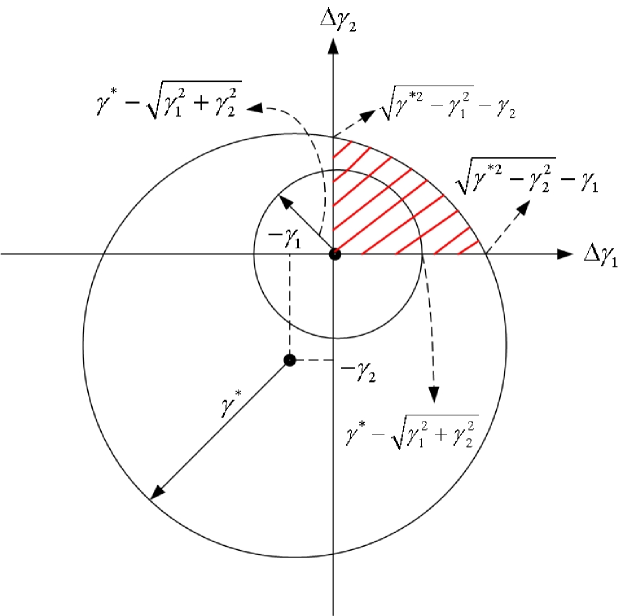
Figure 1: Geometric representation of uncertainty bounds. The admissible region is hachured.

6 Illustrative Example

Consider a system of class $\Sigma_{s}$ and suppose the nonimal system is given as

$$\left[\begin{array}[]{cc}2&3\\ 4&6\\ \end{array}\right]\left[\begin{array}[]{c}\dot{x}_{1}\\ \dot{x}_{2}\\ \end{array}\right]=\left[\begin{array}[]{cc}1&12\\ -6&-15\\ \end{array}\right]\left[\begin{array}[]{c}x_{1}\\ x_{2}\\ \end{array}\right]+\frac{1}{2}\left[\begin{array}[]{c}\sin x_{2}\\ \sin x_{1}\\ \end{array}\right]$$ (181)

$$y=\left[\begin{array}[]{cc}1&0\\ \end{array}\right]\left[\begin{array}[]{c}x_{1}\\ x_{2}\\ \end{array}\right].$$ (185)

We assume the uncertainty and disturbances matrices as follows:

$$M_{1} =\left[\begin{array}[]{cc}0.1&0.1\\ -0.2&0.15\\ \end{array}\right],\ B=\left[\begin{array}[]{c}1\\ 1\\ \end{array}\right],\ N=\left[\begin{array}[]{cc}0.1&0\\ 0&0.1\\ \end{array}\right]$$ (192)

$$M_{2} =\left[\begin{array}[]{cc}-0.25&0.25\\ \end{array}\right],\ \ D=0.2.$$ (194)

The system is globally Lipschitz with $\gamma=0.5$. Now, we design a filter with dynamic structure. Therefore, we have $\mathcal{E}_{1}=I$ and $\mathcal{E}_{2}=0$. Using Corollary 1 with $\mu=0.25$ and $H=0.25I_{2}$, a robust $H_{\infty}$ dynamic filter is obtained as:

$$A_{F} =\left[\begin{array}[]{cc}-70.9676&-44.2097\\ 12.2131&-40.8541\\ \end{array}\right],\ B_{F}=\left[\begin{array}[]{c}4.3896\\ 0.7843\\ \end{array}\right]$$ (199)

$$C_{F} =\left[\begin{array}[]{cc}-0.0057&-0.0043\\ 0.0047&-0.0050\\ \end{array}\right],\ D_{F}=1e-4\times\left[\begin{array}[]{c}-0.3877\\ 0.1026\\ \end{array}\right]$$ (204)

$$\epsilon_{1} =1.2903,\ \ \ \epsilon_{2}=1.4497$$

$$\alpha_{1} =2.1406e-4,\ \ \ \alpha_{2}=1.0024$$

$$\gamma^{*} =0.9988.$$

As mentioned earlier, in order to simulate the system, we need consistent initial conditions. Matrix $\mathbf{E}$ is of rank $1$, thus, the system has $1$ differential equation and $1$ algebraic constraint. The system is currently in the implicit descriptor form. In order to extract the algebraic constraint, we can convert the system into semi-explicit differing algebraic. The matrix $\mathbf{E}$ can be decomposed as:

$$\mathbf{E}=\left[\begin{array}[]{cc}2&3\\ 4&6\\ \end{array}\right]=S\left[\begin{array}[]{cc}1&0\\ 0&0\\ \end{array}\right]T,$$ (209)

where

$$S=\left[\begin{array}[]{cc}1&0\\ 2&1\\ \end{array}\right],\ T=\left[\begin{array}[]{cc}3&2\\ 0&1\\ \end{array}\right].$$ (214)

Now, with the change of variables $\bar{x}=Tx$, the state equations in the original system are rewritten in the semi-explicit form as follows:

$$\left[\begin{array}[]{cc}1&0\\ 0&0\\ \end{array}\right]\left[\begin{array}[]{c}\dot{\bar{x}}_{1}\\ \dot{\bar{x}}_{2}\\ \end{array}\right]= \left[\begin{array}[]{cc}\frac{1}{3}&\frac{34}{3}\\ -\frac{8}{3}&-\frac{101}{3}\\ \end{array}\right]\left[\begin{array}[]{c}\bar{x}_{1}\\ \bar{x}_{2}\\ \end{array}\right]+\left[\begin{array}[]{cc}\frac{1}{2}&0\\ -1&\frac{1}{2}\\ \end{array}\right]\left[\begin{array}[]{c}\sin\bar{x}_{2}\\ \sin(\frac{1}{3}\bar{x}_{1}-\frac{2}{3}\bar{x}_{2})\\ \end{array}\right].$$ (227)

So, the system is clearly decomposed into differential and algebraic parts. The second equation in the above which is:

$$-\frac{8}{3}\bar{x}_{1}-\frac{101}{3}\bar{x}_{2}-sin\bar{x}_{1}+\frac{1}{2}sin(\frac{1}{3}\bar{x}_{1}-\frac{2}{3}\bar{x}_{2})=0,$$

is the algebraic equation which must be satisfied by the initial conditions. A set of consistent initial conditions satisfying the above equation is found as $\bar{x}_{1}(0)=-38.1034,\ \bar{x}_{2}(0)=3.0014$ which corresponds to $x_{1}(0)=-14.7020,\ x_{2}(0)=3.0014$ which in turn corresponds to $z_{1}(0)=-3.6755,z_{2}(0)=0.7503$, where $z=Hx$. Similarly, we find another set of consistent initial conditions for simulating the designed filter. Note that the introduced change of variables is for clarification purposes only to reveal the algebraic constraint which is implicit in the original equations which facilitates calculation of consistent initial conditions, and is not required in the filter design algorithm. Consistent initial conditions could also be calculated using the original equations and in fact, most DAE solvers contain a built-in mechanism for consistent initialization using the descriptor form directly. Figure 2 shows the simulation results of $z$ and $z_{F}$ of the nominal system in the absence of disturbance and uncertainties, where $z_{F}$ is the output of the filter as in (12).

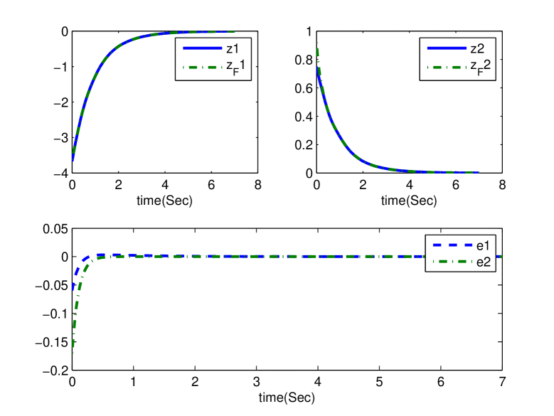
Figure 2: Simulations results of the nominal descriptor system and the $H_{\infty}$ filter

Now suppose an unknown $\mathcal{L}_{2}$ exogenous disturbance signal is affecting the system as $w(t)=50\exp(-0.2t)\cos(5t)$. Figure 3 shows the simulation results of $z$ and $z_{F}$ in the presence of disturbance. As expected, in the presence of disturbance, the observer filter error does not converge to zero (as long as the disturbance exists) but it is kept in the vicinity of zero such that the norm bound $\|e\|\leq\mu\|w\|$ is satisfied. The designed filter guarantees $\mu$ to be at most $0.25$. The actual value of $\mu$ for this simulation is $0.0133$.

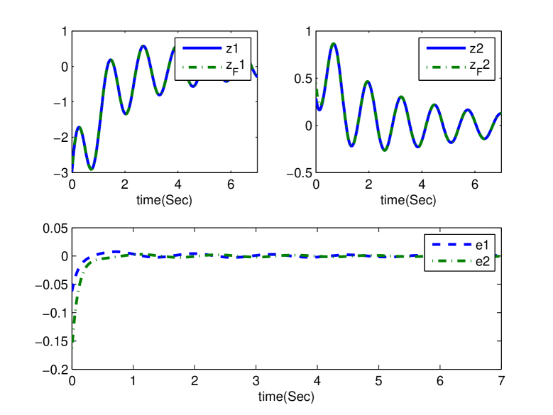
Figure 3: Simulations results of the descriptor system and the $H_{\infty}$ filter in the presence of disturbance

In the next step, we simulate the system in the presence of model uncertainty. An (unknown to the filter) time-varying matrix considered is as $F(t)=diag\left(\frac{t}{t+0.1},\frac{t^{2}+0.1}{t^{2}+1}\right)$. It is easy to verify that $F^{T}(t)F(t)\leq I$ for all $t$. Figure 4 shows the simulation results of $z$ and $z_{F}$ in the presence of model uncertainty. As seen in the figure, the filter is robust against model uncertainty.

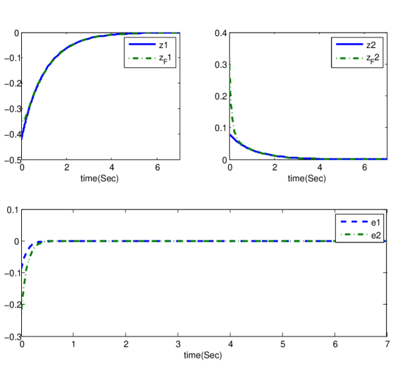
Figure 4: Simulations results of the descriptor system and the $H_{\infty}$ filter in the presence of model uncertainty

Finally, we simulate the system in the presence of both model uncertainty and disturbance. Figure 5 shows the simulation results. The actual value of $\mu$ for this simulation is $0.0187$.

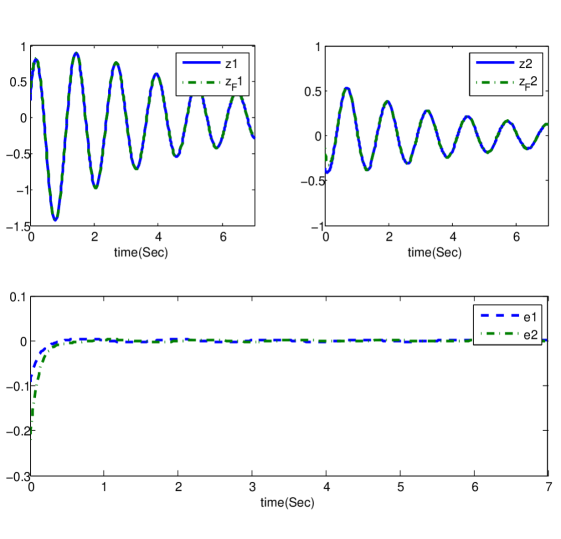
Figure 5: Simulations results of the descriptor system and the $H_{\infty}$ filter in the presence of model uncertainty and disturbance

7 Conclusions and Future Research Directions

In this work, a new nonlinear $H_{\infty}$ dynamical filter design method for a class of nonlinear descriptor uncertain systems is proposed through semidefinite programming and strict LMI optimization. The developed LMIs are linear both in the admissible Lipschitz constant and the disturbance attenuation level allowing both two be an LMI optimization variable. The proposed dynamical structure has more degree of freedom than the conventional static-gain filters and is capable of robustly stabilizing the filter error dynamics for some of those systems for which an static-gain filter cannot be found. In addition, when the static-gain filter also exists, the maximum admissible Lipschitz constant obtained using the proposed dynamical filter structure can be much larger than the at of the static-gain filter. The achieved $H_{\infty}$ filter guarantees asymptotic stability of the error dynamics and is robust against Lipschitz additive nonlinear uncertainty as well as time-varying parametric uncertainty.

In the following we briefly discuss some future research avenues.

energy-to-peak filtering:

As mentioned in the Introduction, in $H_{\infty}$ filtering, the $\mathcal{L}_{2}$ gain from the exogenous disturbance to the filter error is guaranteed to be less than a prespecified level, making the underlying $\mathcal{L}_{2}$ gain minimization an energy-to-energy performance criterion. An alternative approach is the so-called $\mathcal{L}_{2}-\mathcal{L}_{\infty}$ filtering. In $\mathcal{L}_{2}-\mathcal{L}_{\infty}$ filtering, the ratio of the peak value of the error ($\mathcal{L}_{\infty}$ norm) to the energy of disturbance ($\mathcal{L}_{2}$ norm) is considered, therefore, conforming an energy-to-peak performance criterion. The tools and methods provided in this work can be used to solve the robust $\mathcal{L}_{2}-\mathcal{L}_{\infty}$ filtering problem for the studied class of nonlinear descriptor systems.

mixed $H_{2}/H_{\infty}$ filtering:

One the main advantages of $H_{\infty}$ approach is that it does not require any knowledge about the statistics of noise. It works for every finite energy signal. The noise terms may be random with possibly unknown statistics, or they may be deterministic. If the statistics of noise are known, Kalman filtering (i.e. $H_{2}$) approaches can be used. However, estimating the statistics of noise is a difficult task and the representation of disturbances by white noise processes are often unrealistic. That was one the main motives that $H_{\infty}$ approaches developed at the first place. Nevertheless, the prior knowledge about the statistics of disturbance can be utilized to set up a mixed $H_{2}/H_{\infty}$ performance criterion.

uncertainty in the mass matrix:

To the best of the author’s knowledge, in all works on nonlinear uncertain descriptor systems (including this work), the mass matrix $\mathbf{E}$ is assumed to be fully known. This is required because the matrix $\mathbf{E}$ participates in the construction of the generalized Lyapunov function. For models with unstructured uncertainty, this is not a big deal. However, for models with structured parametric uncertainty, there might be cases that an intrinsic uncertainty is associated with the elements of $\mathbf{E}$ (e.g. due to presence of uncertain parameters in $\mathbf{E}$), which cannot be incorporated into $A$ and $C$. Therefore, considering a $\Delta\mathbf{E}$ might become inevitable. This is currently an open problem.

References

• [1] Masoud Abbaszadeh and Horacio J. Marquez. Robust $H_{\infty}$ observer design for a class of nonlinear uncertain systems via convex optimization. Proceedings of the 2007 American Control Conference, New York, U.S.A., pages 1699–1704.
• [2] Masoud Abbaszadeh and Horacio J Marquez. LMI optimization approach to robust $H_{\infty}$ filtering for discrete-time nonlinear uncertain systems. In American Control Conference, 2008, pages 1905–1910. IEEE, 2008.
• [3] Masoud Abbaszadeh and Horacio J. Marquez. Robust $H_{\infty}$ observer design for sampled-data Lipschitz nonlinear systems with exact and Euler approximate models. Automatica, 44(3):799–806, 2008.
• [4] Masoud Abbaszadeh and Horacio J. Marquez. LMI optimization approach to robust $H_{\infty}$ observer design and static output feedback stabilization for discrete-time nonlinear uncertain systems. International Journal of Robust and Nonlinear Control, 19(3):313–340, 2009.
• [5] Masoud Abbaszadeh and Horacio J Marquez. A generalized framework for robust nonlinear $H_{\infty}$ filtering of lipschitz descriptor systems with parametric and nonlinear uncertainties. Automatica, 48(5):894–900, 2012.
• [6] O. Agamennonia, I. Skrjanc, M. Lepetic, H. Chiacchiarinic, and D. Matko. Nonlinear uncertainty model of a magnetic suspension system. Mathematical and Computer Modelling, 40(9-10):1075–1087, 2007.
• [7] B. Boulkroune, M. Darouach, and M. Zasadzinski. Moving horizon state estimation for linear discrete-time singular systems. Control Theory Applications, IET, 4(3):339 –350, march 2010.
• [8] B. Boulkroune and A. Zemouche. Robust fault diagnosis for a class of nonlinear descriptor systems. In Control and Fault-Tolerant Systems (SysTol), 2010 Conference on, pages 335 –340, oct. 2010.
• [9] M. Boutayeb and M. Darouach. Observers design for nonlinear descriptor systems. Proceedings of the IEEE Conference on Decision and Control, 3:2369–2374, 1995.
• [10] F.E. Cellier and E. Kofman. Continuous System Simulation. Springer, 2006.
• [11] L. Dai. Singular control systems, volume 118 of Lecture Notes on Control and Information Sciences. Sprinter, 1989.
• [12] M. Darouach and L. Boutat-Baddas. Observers for lipschitz nonlinear descriptor systems: Application to unknown inputs systems. In Control and Automation, 2008 16th Mediterranean Conference on, pages 1369 –1374, june 2008.
• [13] M. Darouach and M. Boutayeb. Design of observers for descriptor systems. IEEE Transactions on Automatic Control, 40(7):1323–1327, 1995.
• [14] M. Darouach, M. Zasadzinski, and M. Hayar. Reduced-order observer design for descriptor systems with unknown inputs. IEEE Transactions on Automatic Control, 41(7):1068–1072, 1996.
• [15] Carlos E. de Souza, Lihua Xie, and Youyi Wang. $H_{\infty}$ filtering for a class of uncertain nonlinear systems. Systems and Control Letters, 20(6):419–426, 1993.
• [16] Peter Fritzson. Principles of Object-Oriented Modeling and Simulation with Modelica 2.1. Wiley-IEEE Press, 2004.
• [17] R. A. Horn and C. R. Johnson. Matrix Analysis. Cambrige University Press, 1985.
• [18] M. Hou and P. C. Muller. Observer design for descriptor systems. IEEE Transactions on Automatic Control, 44(1):164–169, 1999.
• [19] J. Y. Ishihara and M. H. Terra. On the Lyapunov theorem for singular systems. IEEE Transactions on Automatic Control, 47(11):1926–1930, 2002.
• [20] Pramod P. Khargonekar, Ian R. Petersen, and Kemin Zhou. Robust stabilization of uncertain linear systems: Quadratic stabilizability and $H_{\infty}$ control theory. IEEE Transactions on Automatic Control, 35(3):356–361, 1990.
• [21] R.L. Kosut. Nonlinear uncertainty model unfalsification. In American Control Conference, 1997. Proceedings of the 1997, volume 3, pages 2098–2102, 1997.
• [22] J. Lofberg. YALMIP : A toolbox for modeling and optimization in MATLAB. 2004.
• [23] G. Lu and D. W. C. Ho. Full-order and reduced-order observers for Lipschitz descriptor systems: The unified LMI approach. IEEE Transactions on Circuits and Systems II: Express Briefs, 53(7), 2006.
• [24] R. Luck and J. W. Stevens. A simple numerical procedure for estimating nonlinear uncertainty propagation. ISA Transations, 43(4):491–497, 2004.
• [25] H. J. Marquez. Nonlinear Control Systems: Analysis and Design. Wiley, NY, 2003.
• [26] I. Masubuchi, Y. Kamitane, A. Ohara, and N. Suda. $H_{\infty}$ control for descriptor systems: A matrix inequalities approach. Automatica, 33(4):669–673, 1997.
• [27] Constantinos C. Pantelides. The consistent initialization of differential-algebraic systems. SIAM Journal on Scientific Computing, 9(2):219–231, 1988.
• [28] Obaid Ur Rehman, Baris Fidan, and Ian R. Petersen. Uncertainty modeling and robust minimax LQR control of multivariable nonlinear systems with application to hypersonic flight. Asian Journal of Control, 2011.
• [29] McKenna L. Robertsa, James W. Stevensa, , and Rogelio Luck. Evaluation of parameter effects in estimating non-linear uncertainty propagation. Measurement, 40(1):15–20, 2007.
• [30] E. Feron S. Boyd, L. El Ghaoui and V. Balakrishnan. Linear matrix inequalities in system and control theory. SIAM, PA, 1994.
• [31] D. N. Shields. Observer design and detection for nonlinear descriptor systems. International Journal of Control, 67(2):153–168, 1997.
• [32] Jos F. Sturm. SeDuMi. 2001.
• [33] Eiho Uezato and Masao Ikeda. Strict LMI conditions for stability, robust stabilization, and $H_{\infty}$ control of descriptor systems. Proceedings of the 38th IEEE Conference on Decision and Control, 4:4092–4097, 1999.
• [34] He-Sheng Wang, Chee-Fai Yung, and Fen-Ren Chang. $H_{\infty}$ control for Nonlinear Descriptor Systems, volume 326 of Lecture Notes in Control and Information Sciences. Springer, 2006.
• [35] Youyi Wang, Lihua Xie, and Carlos E. de Souza. Robust control of a class of uncertain nonlinear systems. Systems and Control Letters, 19(2):139–149, 1992.
• [36] G. Zimmer and J. Meier. On observing nonlinear descriptor systems. Systems and Control Letters, 32(1):43–48, 1997.