Life and death of stationary linear response in anomalous continuous time random walk dynamics

Abstract

Linear theory of stationary response in systems at thermal equilibrium requires to find equilibrium correlation function of unperturbed responding system. Studies of the response of the systems exhibiting anomalously slow dynamics are often based on the continuous time random walk description (CTRW) with divergent mean waiting times. The bulk of the literature on anomalous response contains linear response functions like one by Cole-Cole calculated from such a CTRW theory and applied to systems at thermal equilibrium. Here we show within a fairly simple and general model that for the systems with divergent mean waiting times the stationary response at thermal equilibrium is absent, in accordance with some recent studies. The absence of such stationary response (or dying to zero non-stationary response in aging experiments) would confirm CTRW with divergent mean waiting times as underlying physical relaxation mechanism, but reject it otherwise. We show that the absence of stationary response is closely related to the breaking of ergodicity of the corresponding dynamical variable. As an important new result, we derive a generalized Cole-Cole response within ergodic CTRW dynamics with finite waiting time. Moreover, we provide a physically reasonable explanation of the origin and wide presence of $1/f$ noise in condensed matter for ergodic dynamics close to normal, rather than strongly deviating.

I Introduction

Theories of anomalous diffusion and transport abound KLM , including continuous time random walks (CTRW)Shlesinger ; Scher ; Hughes and related fractional Fokker-Planck equations Metzler , generalized Langevin equations Kubo ; Coffey ; WeissBook ; Goychuk12 , anomalous kinetic equations of the (linear) Boltzmann equation type Balescu ; BarkaiSilbey , hopping and continuous dynamics in disordered and fractal media Bouchaud ; Havlin , etc. Often it is not clear from the experimental results which theory works better for the case of study. In particular, theory of anomalous response is often based on CTRW with divergent mean residence times (MRTs). Often it is seen as a proper explanation of the physical origin of all major anomalous response functions, including Cole-Cole response Cole featuring the so-called fast or $\beta-$relaxation in complex liquids and glasses. The latter one is relatively fast (lasting from pico- to milliseconds, even if it follows to a power law), and the corresponding response quickly becomes stationary on the time scale of observations. It is followed by $\alpha-$relaxation, which is often described by Kohlrausch-Williams-Watts stretched exponential dependence, or even better Lunken1 by the Cole-Davidson relaxation law. $\alpha-$relaxation extends up to $10^{4}-10^{6}$ seconds in a typical aging experiment Lunken1 ; Oukris , until a stationary response regime is reached Lunken1 ; Oukris ; Lunken .

Stationary response requires to calculate stationary autocorrelation function (ACF). If to do this properly for CTRW with divergent mean residence times, it becomes clear that such a response is absent, because the corresponding stationary ACF does not decay at all. This in turn indicates the breaking of ergodicity in accordance with the Slutsky theorem Papoulis . Non-ergodic CTRW cannot respond to stationary perturbations in a very long run. Its response must die to zero, which invalidates a part of the CTRW based theories of anomalous stationary response, when applied to physical systems at thermal equilibrium. We discuss these subtleties below within a sufficiently simple and generic model.

II Theory and Model

Linear response theory has been put by Kubo on the firm statistic-mechanical foundation Kubo ; Zwanzig ; Marconi . Consider a physical system with dynamical variable $x(t)$, say coordinate of a particle moving in a multistable potential in a dissipative environment. It exhibits stochastic dynamics (here classical) due to thermal agitations of the medium at temperature $T$, with the ensemble average $\langle x(t)\rangle_{\rm st}=x_{\rm eq}$ (we bear in mind many independent particles). The system is at thermal equilibrium. One applies a periodic driving force $f(t)=f_{0}\cos(\Omega t)$ with frequency $\Omega$ and amplitude $f_{0}$ linearly coupled to the dynamical variable $x(t)$, with perturbation energy $-fx$. The mean deviation from equilibrium, $\langle\delta x(t)\rangle=\langle x(t)\rangle-x_{\rm eq}$, responds generally to the driving switched on at the time $t_{0}=0$ with some delay Kubo ; Zwanzig ,

$$\langle\delta x(t)\rangle=\int_{0}^{t}\chi(t-t^{\prime})f(t^{\prime})dt^{\prime},$$ (1)

where $\chi(t-t^{\prime})$ is the linear response function (LRF), and the upper integration limit $t$ reflects causality. For any physical system at thermal equilibrium and weakly perturbed by driving, LRF can depend only on the difference of time arguments. Stationary response to the periodic signal reads ($t\to\infty$)

$$\langle\delta x(t)\rangle_{\rm as}=f_{0}|\hat{\chi}(\Omega)|\cos(\Omega t-\varphi),$$ (2)

where $\hat{\chi}(\omega)=\int_{-\infty}^{\infty}e^{i\omega t}\chi(t)dt=\int_{0}^{\infty}e^{i\omega t}\chi(t)dt$ is the (Laplace-)Fourier transform of $\chi(t)$ ($\chi(t)=0$ for $t<0$ due to causality), and $\varphi=\tan^{-1}\left({\rm Im}\hat{\chi}(\omega)/{\rm Re}\hat{\chi}(\omega)\right)$ is the phase lag. Kubo derived from microscopic Hamiltonian dynamics under fairly general conditions that such stationary LRF is related to equilibrium autocorrelation function, or rather covariance $K(t)=\langle\delta x(t)\delta x(0)\rangle_{\rm eq}$ of the variable $x(t)$ as Kubo ; Zwanzig ; Marconi

$$\chi(t)=-\frac{H(t)}{k_{B}T}\frac{d}{dt}\langle\delta x(t)\delta x(0)\rangle_{\rm eq}\;,$$ (3)

where $H(t)$ is the Heaviside step function. This fundamental result in statistical physics is known as classical fluctuation-dissipation theorem (FDT) in the time domain. Stationary response is related to the equilibrium autocorrelation function which must be stationary. A generalization of this result to a nonstationary, e.g. aging environment, or in the presence of steady state nonequilibrium fluxes in the unperturbed state (non-equilibrium steady state – NESS) is not trivial. Especially, the systems exhibiting non-Gaussian anomalous diffusion demonstrate profound deviations from equilibrium FDT behavior in NESS Villamaina ; Gradenigo . Non-equilibrium FDT was developed primarily for the systems with underlying Markovian dynamics Cugliandolo ; Lippielo . It allows, for example, to rationalize the NESS response of anomalous 1d subdiffusive dynamics to a small additional tilt on a comb lattice Villamaina . This dynamics is embedded as 2d Markovian dynamics Villamaina . A generalization to intrinsically non-Markovian dynamics is yet to be done. In the present work, we are focusing on a standard response of unperturbed systems being at thermal equilibrium, without dissipative fluxes present.

Specifically, our focus is on anomalous non-Debye type response featuring many materials. As an important example, famous Cole-Cole response function Cole reads (setting the high-frequency component $\hat{\chi}(\infty)$ to zero)

$$\hat{\chi}(\omega)=\frac{\chi_{0}}{1+(-i\omega\tau_{r})^{\alpha}}$$ (4)

in the frequency domain, with static $\chi_{0}=\langle\delta x^{2}(0)\rangle_{\rm eq}/(k_{B}T)$ and $0<\alpha<1$. The Cole-Cole response corresponds to the Mittag-Leffler relaxation Metzler ; Gorenflo of the autocorrelation function

$$K(t)=\langle\delta x^{2}(0)\rangle_{\rm eq}E_{\alpha}[-(t/\tau_{r})^{\alpha}],$$ (5)

where $E_{\alpha}[z]=\sum_{n=0}^{\infty}z^{n}/\Gamma(\alpha n+1)$ is Mittag-Leffler function Metzler ; Gorenflo and $\tau_{r}$ is (anomalous) relaxation time, which in the range of from picoseconds to milliseconds for various materials Cole . If a constant signal $f_{0}=const$ is switched on at $t_{0}=0$, then the time-dependent response in accordance with FDT is

$$\langle\delta x(t)\rangle=\frac{f_{0}}{k_{B}T}\left[K(0)-K(t)\right]\;.$$ (6)

It starts from zero and approaches the asymptotical value $\langle\delta x(\infty)\rangle=\frac{f_{0}}{k_{B}T}\langle\delta x^{2}(0)\rangle_{\rm eq}$, if $K(t)\to 0$ with $t\to\infty$.

II.1 CTRW model

We model further the thermal dynamics of $x(t)$ by a non-Markovian (semi-Markovian) CTRW of the following type. There are $N$ localized states $x_{i}$ which are populated with stationary probabilities $p_{i}$. Scattering events due to a thermal agitation are not correlated and distributed in time with the waiting time density (WTD) $\psi(\tau)$, which is normalized and has a finite mean time $\langle\tau\rangle$ between two subsequent events. Scattering can lead to any other state, but the particle can remain also in the same state. The finiteness of $\langle\tau\rangle$ is crucial for calculating the stationary ACF. Then, we can study the response of our system in the limit $\langle\tau\rangle\to\infty$, after the stationary ACF $K(t)$ is found and not before, overcoming thereby the common fallacy done in huge many previous works (they are simply not based on the correct stationary ACF). The transition probability from the state $j$ to the state $i$ is $T_{ij}=p_{i}$, i.e. it corresponds to the statistical weight of the next trapping state. Such a CTRW is a particular version of separable CTRW by Montroll and Weiss Hughes . This is a toy model, but the main features are expected to be generic. To calculate the stationary and equilibrium averages the distribution of the first residence time is required Tunaley ; GH03 ; GH05 . It is well-known to be Cox $\psi^{(0)}(\tau)=\Phi(\tau)/\langle\tau\rangle$ (see also below in Sec. II.4 for a derivation of this result), where $\Phi(\tau)=\int_{\tau}^{\infty}\psi(\tau^{\prime})d\tau^{\prime}$ is survival probability. The survival probability for the first sojourn without scattering events is $\Phi^{(0)}(\tau)=\int_{\tau}^{\infty}\psi^{(0)}(\tau^{\prime})d\tau^{\prime}=\int_{\tau}^{\infty}\Phi(\tau^{\prime})d\tau^{\prime}/\langle\tau\rangle$. It plays the central role. We show in Appendix that

$$K(t)=\langle\delta x^{2}(0)\rangle_{\rm eq}\Phi^{(0)}(t)$$ (7)

within this fully decoupled CTRW model.

Now we can ask the question if such a probability density $\psi(\tau)$ exists within this model that we can obtain the Cole-Cole response exactly. The answer is no. Indeed, the Laplace transform of $\Phi^{(0)}(t)$ is related to the Laplace transform of survival probability $\tilde{\Phi}(s)$ as

$$\tilde{\Phi}^{(0)}(s)=\frac{1}{s}\left[1-\frac{\Phi(s)}{\langle\tau\rangle}\right]\;.$$ (8)

For the Mittag-Leffler relaxation $\tilde{\Phi}^{(0)}(s)=\tau_{r}/[s\tau_{r}+(s\tau_{r})^{1-\alpha}]$. From this and (8), $\tilde{\Phi}(s)=\tau_{r}/(1+(s\tau_{r})^{\alpha})$, which does not correspond to any survival probability since $\lim_{t\to 0}\Phi(t)=\lim_{s\to\infty}s\tilde{\Phi}(s)=\infty$, and not $\Phi(0)=1$, as must be. Remarkably, within the framework of Langevin dynamics with memory the Cole-Cole response is easily reproduced by fractional overdamped Langevin dynamics in parabolic potential Goychuk07 .

From Eqs. (7) and (8) it follows immediately in the formal limit $\langle\tau\rangle\to\infty$ that $\tilde{K}(s)\to\langle\delta x^{2}(0)\rangle_{\rm eq}/s$ for any WTD, which means that

$$K(t)=\langle\delta x^{2}(0)\rangle_{\rm eq}\;.$$ (9)

It does not decay at all! From this in (3) it follows immediately that stationary response is absent exactly,

$$\chi(t)=0\;.$$ (10)

The “no stationary response” theorem for a rather general class of processes with infinite mean residence time is thus proven. It agrees with the death of response found earlier for other non-ergodic CTRW dynamics Barbi ; Sokolov06 ; H07 ; West ; Allegrini09 . In fact, it follows at once by the fluctuation-dissipation theorem (3) from nonergodicity of any process $x(t)$ with divergent mean residence times BarkaiMargolin . The breaking of ergodicity in turn follows by the virtue of Slutsky theorem from nondecaying character of stationary autocorrelation function Papoulis . Non-ergodic system with $\langle\tau\rangle=\infty$ cannot respond stationary to a stationary (e.g. periodic) signal, and the corresponding theories of linear response at thermal equilibrium are deeply flawed. However, it is more instructive to investigate the way how the stationary response becomes increasingly suppressed with increasing $\langle\tau\rangle$. Two particular models are interesting in this respect.

II.2 Tempered distribution

The first model corresponds to the Mittag-Leffler density tempered by introduction of an exponential cutoff Saichev . The corresponding survival probability is $\Phi(t)=E_{\alpha}[-r_{\alpha}t^{\alpha}]\exp(-rt)$, where $r_{\alpha}$ is fractional rate and $r$ is a cutoff rate. All the moments then become finite. The survival probability has Laplace transform

$$\tilde{\Phi}(s)=\frac{1}{s+r+r_{\alpha}(s+r)^{1-\alpha}}\,.$$ (11)

The mean time is $\tilde{\Phi}(0)=1/[r+r_{\alpha}r^{1-\alpha}]=\langle\tau\rangle$, and

$$\tilde{K}(s)=\frac{\langle\delta x^{2}(0)\rangle_{\rm eq}}{s}\frac{s+r_{\alpha}(s+r)^{1-\alpha}-r_{\alpha}r^{1-\alpha}}{s+r+r_{\alpha}(s+r)^{1-\alpha}}\,.$$ (12)

Clearly, it also exhibits the generic death of stationary response in the limit $\langle\tau\rangle\to\infty$.

We shall not elaborated this model in more detail here, bur rather focus on a very different model with finite $\langle\tau\rangle$, but divergent higher moments. It exhibits a number of other surprising and interesting features.

II.3 Mixing normal and anomalous relaxation

We assume that transition events can occur either with normal rate $r$, or with some fractional rate $r_{\alpha_{i}}$ ($0<\alpha_{i}<1$) intermittently through $m+1$ independent relaxation channels. This yields the following survival probability Goychuk12PRE ,

$$\tilde{\Phi}(s)=\frac{1}{s+r+\sum_{j=1}^{m}r_{\alpha_{j}}s^{1-\alpha_{j}}}\;,$$ (13)

which can also be written as

$$\tilde{\Phi}(s)=\frac{\langle\tau\rangle}{1+\langle\tau\rangle s+\sum_{j=1}^{m}(\tau_{j}s)^{1-\alpha_{j}}}\;,$$ (14)

where $\langle\tau\rangle=\tilde{\Phi}(0)=1/r$ is the mean relaxation time (defined exclusively by the normal relaxation channel) and the time constants $\tau_{i}=(r_{\alpha_{i}}\langle\tau\rangle)^{1/(1-\alpha_{i})}$ provide the spectrum of anomalous relaxation times. Specifying the generalized master equation (GME) by Kenkre, Montroll, and Shlesinger Kenkre for this model (see e.g. Appendix in Ref. Goychuk04 for a general derivation from the trajectory perspective) yields fractional relaxation equation

$$\dot{p}_{i}(t) = -\sum_{j=0}^{m}r_{\alpha_{j}}\sideset{{}_{0}}{{}_{t}}{\mathop{\hat{D}}^{1-\alpha_{j}}}\left[p_{i}(t)-p_{i}\right],$$ (15)

where

$$\sideset{{}_{t_{0}}}{{}_{t}}{\mathop{\hat{D}}^{1-\alpha}}p(t):=\frac{1}{\Gamma(\alpha)}\frac{d}{dt}\int_{t_{0}}^{t}dt^{\prime}\frac{p(t^{\prime})}{(t-t^{\prime})^{1-\alpha}},$$ (16)

defines the operator of fractional Riemann-Liouville derivative of the order $1-\alpha$ Metzler ; Gorenflo . Eq. (15) belongs to a general class of GMEs with distributed fractional derivatives distributed . One relaxation channel must be normal, $\alpha_{0}=1$, $r_{\alpha_{0}}=r$ for ergodic process. Evolution of state probabilities $p_{i}(t)$ become completely decoupled because of our choice of the transition probabilities, $T_{ij}=p_{i}$. From Eq. (15), $p_{i}$ are obviously the stationary probabilities, $\lim_{t\to\infty}p_{i}(t)=p_{i}^{(\rm st)}=p_{i}$, which is not immediately obvious from the trajectory description.

For normal relaxation, our choice of model corresponds to a very popular textbook model of single relaxation time $\langle\tau\rangle$, which does not depend on the particular state. It is often used as the simplest approximation in studying various kinetic equations. By the same token, anomalous relaxation times also do not depend on the particular state within the model considered. Notice, however, that GME (15) cannot be used to find the stationary ACF (7). Its direct use would be namely the typical fallacy which plagued many earlier works. One must proceed differently, see in Appendix for details.

For the simplest nontrivial case $m=1$ with $\alpha_{1}=\alpha$, $\tau_{r}=\tau_{1}$, and in the parameter regime $\langle\tau\rangle\ll\tau_{r}$, $\Phi(t)\approx E_{\alpha}(-r_{\alpha}t^{\alpha})$, on the time scale $t\ll\tau_{r}$. It corresponds to the same WTD as in the basic CTRW model with divergent $\langle\tau\rangle$. Hence, for $t\ll\tau_{\alpha}=r_{\alpha}^{-1/\alpha}$, $\psi(\tau)\propto\tau^{-1+\alpha}$. This initial power law corresponds to the initially stretched exponential survival probability $\Phi(t)\approx\exp(-r_{\alpha}t^{\alpha}/\Gamma(1+\alpha))$. Then, intermediate power law follows, $\psi(\tau)\propto\tau^{-1-\alpha}$, for $\tau$ within the range

$$\tau_{\alpha}=[\langle\tau\rangle/\tau_{r}]^{1/\alpha}\tau_{r}\ll\tau\ll\tau_{r}\;,$$ (17)

i.e. over $[\tau_{r}/\langle\tau\rangle]^{1/\alpha}$ intermediate time decades. For $\tau\gg\tau_{r}$, it further changes into the asymptotic power law $\psi(\tau)\propto\tau^{-3+\alpha}$ Goychuk12PRE . Interestingly enough, introduction of a finite $\langle\tau\rangle$ results into a sufficiently strong power law decay for $\tau>\tau_{r}$. The parameter $\tau_{r}$ plays thus the role of a cutoff time, though the cutoff character is very different from the model of exponentially tempered distribution. The latter one has an exponential cutoff for $t\gg 1/r$. The important parameter regime, $\langle\tau\rangle\ll\tau_{r}$, is depicted in Fig. 1. Notice, however, that for $\langle\tau\rangle\sim\tau_{r}$, the intermediate power law first disappears, and for $\langle\tau\rangle\gg\tau_{r}$ it transforms into intermediate exponential decay (like one in Fig. 2,b).

Figure 1: Dependence of probability density $\psi(\tau)$ on time (in units of $\tau_{r}$) for $\langle\tau\rangle=0.01$ and $\alpha=0.25$ exhibits three different power laws, $\tau^{-1+\alpha}$, $\tau^{-1-\alpha}$, $\tau^{-3+\alpha}$, in the parameter regime $\langle\tau\rangle\ll\tau_{r}$.

The Laplace-transformed stationary ACF of this model reads

$$\tilde{K}(s)=\langle\delta x^{2}(0)\rangle_{\rm eq}\frac{1+\sum_{i=1}^{m}r_{\alpha_{i}}s^{-\alpha_{i}}}{s+r+\sum_{i=1}^{m}r_{\alpha_{i}}s^{1-\alpha_{i}}},$$ (18)

from which it becomes immediately clear that in the limit $r=1/\langle\tau\rangle\to 0$, the limiting stationary ACF is simply constant, as in Eq. (9). The stationary response is absent.

Furthermore, the response function in Laplace domain follows as

$$\tilde{\chi}(s)=\frac{\chi_{0}}{1+\langle\tau\rangle s+\sum_{i=1}^{m}(\tau_{i}s)^{1-\alpha_{i}}}.$$ (19)

In frequency domain it is $\hat{\chi}(\omega)=\tilde{\chi}(-i\omega)$. We have thus a nice and nontrivial generalization of Cole-Cole response function which includes one normal relaxation time $\langle\tau\rangle$ and $m$ anomalous. It provides a very rich model of anomalous response based on ergodic CTRW dynamics with finite mean waiting time. We consider further the particular case of one anomalous relaxation channel, $m=1$. Then, the Cole-Cole response with index $1-\alpha$ instead of $\alpha$ is reproduced in the limit $\langle\tau\rangle\to 0$ at fixed anomalous relaxation time $\tau_{r}=\tau_{1}$. Strikingly enough, this is the opposite limit with respect to one considered in the theory of CTRW with infinite $\langle\tau\rangle=\infty$. Indeed, for sufficiently small $\langle\tau\rangle\ll\tau_{r}$, $K(t)\approx\langle\delta x^{2}(0)\rangle_{\rm eq}E_{1-\alpha}[-(t/\tau_{r})^{1-\alpha}]$, see in Fig. 2. This corresponds to the Cole-Cole response with exponent $1-\alpha$ providing a very important result: stationary Cole-Cole response emerges within the CTRW approach if there exists a very fast normal relaxation channel acting in parallel to the anomalous one and making the mean transition times finite. In striking contrast to the traditional CTRW models based on $\psi(\tau)\propto\tau^{-1-\alpha}$ dependence with divergent mean residence times our approach yields the Cole-Cole response with exponent $1-\alpha$ instead of $\alpha$.

Furthermore, it is instructive to see how $K(t)$ and the response function $\hat{\chi}(\omega)$, behave for large but finite $\langle\tau\rangle=1/r$ with $\tau_{r}$ kept constant. Autocorrelation function is plotted in Fig. 2 for $\alpha=0.5$. Notice that it has a heavy power law tail $K(t)\propto 1/t^{1-\alpha}$, onset of which moves to larger $t$ with the increase of $\langle\tau\rangle$. For very large $\langle\tau\rangle\gg\tau_{r}$, the initial decay is nearly exponential, $K(t)\approx\langle\delta x^{2}(0)\rangle_{\rm eq}\exp(-t/\langle\tau\rangle)$. With this in Eq. (6), one can clearly see that on the time scale $t\ll\langle\tau\rangle$, the response of stationary equilibrium environment is not realized, being increasingly suppressed with the increase of $\langle\tau\rangle$. Time-dependent signals with frequencies smaller than a corner frequency $\omega_{c}=1/\langle\tau\rangle$ should be regarded as slow. However, the response to them (even if it does exist asymptotically!) cannot be detected in noisy background as we shall clarify soon. The dependence on $\alpha$ is very important and remarkable. It is very different from one of CTRW theory with infinite mean time. Basically, we have $\alpha$ instead of $1-\alpha$. This means that with $\alpha$ close to one, e.g. $\alpha=0.95$, the corresponding power noise spectrum

$$S(\omega) =2{\rm Re}[\tilde{K}(-i\omega)]$$ (20)

$$=2\langle\delta x^{2}(0)\rangle_{\rm eq}\frac{\tau_{r}(\omega\tau_{r})^{\alpha}\cos(\frac{\alpha\pi}{2})+\langle\tau\rangle(\omega\tau_{r})^{2\alpha}}{A(\omega)},$$

where

$$A(\omega)=(\omega\tau_{r})^{2\alpha}+\left(\frac{\langle\tau\rangle}{\tau_{r}}\right)^{2}(\omega\tau_{r})^{2(1+\alpha)}+(\omega\tau_{r})^{2}$$

$$+2\frac{\langle\tau\rangle}{\tau_{r}}(\omega\tau_{r})^{\alpha+2}\cos\left(\frac{\alpha\pi}{2}\right)+2(\omega\tau_{r})^{\alpha+1}\sin\left(\frac{\alpha\pi}{2}\right),$$ (21)

becomes very close to $1/f$ noise at small frequencies, $S(\omega)\propto 1/\omega^{\alpha}$, see in Fig. 3. Notice that the closer the anomalous relaxation channel to the normal one the closer the power spectrum becomes to one of $1/f$ noise! This provides a very nice and physically plausible explanation of the wide presence of $1/f$ noise in condensed matter Weisman . The second relaxation channel must be most similar to the normal one and not mostly deviating.

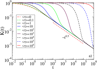
Figure 2: Normalized correlation function (in units of $\langle\delta x^{2}(0)\rangle_{\rm eq}$) on time (in units of $\tau_{r}$) for different $\langle\tau\rangle$ and $\alpha=0.5$. The tail is always $K(t)\propto t^{-1+\alpha}$, see in part a). Decay of correlations is dramatically delayed with the increase of $\langle\tau\rangle$. Initially, it is exponential for $\langle\tau\rangle\gg\tau_{r}$, $K(t)\approx\langle\delta x^{2}(0)\rangle_{\rm eq}\exp(-t/\langle\tau\rangle)$, as part b) shows. The limit $\langle\tau\rangle\to 0$, corresponds to the Mittag-Leffler decay of correlations, $K(t)\approx\langle\delta x^{2}(0)\rangle_{\rm eq}E_{1-\alpha}[-(t/\tau_{r})^{1-\alpha}]$ and Cole-Cole response. Part b) represents some of the curves in part a) on semi-logarithmic plot revealing initial exponential decay for large $\langle\tau\rangle$.

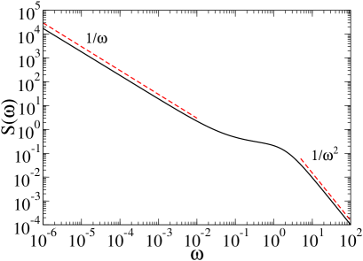
Figure 3: Power spectrum $S(\omega)$ (in units of $2\langle\delta x^{2}(0)\rangle_{\rm eq}\tau_{r}$) on circular frequency (in units of $\tau_{r}^{-1}$) for $\alpha=0.95$ and $\langle\tau\rangle=\tau_{r}$.

Furthermore, real and imaginary parts of the response function are

$${\rm Re}[\chi(\omega)] =\chi_{0}\frac{(\omega\tau_{r})^{1+\alpha}\sin(\frac{\alpha\pi}{2})+(\omega\tau_{r})^{2\alpha}}{A(\omega)},$$ (22)

and

$${\rm Im}[\chi(\omega)] =\frac{1}{2k_{B}T}\omega S(\omega)$$ (24)

$$=\chi_{0}\frac{(\omega\tau_{r})^{1+\alpha}\cos(\frac{\alpha\pi}{2})+\frac{\langle\tau\rangle}{\tau_{r}}(\omega\tau_{r})^{2\alpha+1}}{A(\omega)},$$

correspondingly. Notice that Eq. (24) is nothing else the classical FDT in the frequency domain. This is an exact relation justifying the given name FDT, since ${\rm Im}[\chi(\omega)]$ is related to dissipation losses. It cannot be violated at thermal equilibrium for classical dynamics. The absolute value of the response function measuring the output-to-input ratio of periodic signal amplitude is

$$|\chi(\omega)|=\chi_{0}\frac{(\omega\tau_{r})^{\alpha}}{\sqrt{A(\omega)}},$$ (25)

and the phase lag given by

$$\tan\varphi=\frac{(\omega\tau_{r})^{1+\alpha}\cos(\frac{\alpha\pi}{2})+\frac{\langle\tau\rangle}{\tau_{r}}(\omega\tau_{r})^{2\alpha+1}}{(\omega\tau_{r})^{1+\alpha}\sin(\frac{\alpha\pi}{2})+(\omega\tau_{r})^{2\alpha}}\;.$$ (26)

For slow signals with frequencies $\omega\ll\omega_{c}$, $|\chi(\omega)|\approx\chi_{0}$. This corresponds to quasi-static response. The response to such slow periodic signals is present, as this result shows. However, this does not mean that it can be detected. The signal-to-noise ratio (SNR), $R_{\rm SN}(\omega)=\pi f_{0}^{2}|\chi(\omega)|^{2}/S(\omega)$ which measures the ratio of spectral amplitude of signal to the spectral power of noise at the same frequency is important to determine whether the signal can in principle be detected in the noise background, or not SR . For the discussed model,

$$R_{\rm SN}(\omega) =B\frac{(\omega\tau_{r})^{2\alpha}}{\tau_{r}(\omega\tau_{r})^{\alpha}\cos(\frac{\alpha\pi}{2})+\langle\tau\rangle(\omega\tau_{r})^{2\alpha}},$$ (27)

where $B=(\pi/2)f_{0}^{2}\langle\delta x^{2}(0)\rangle_{\rm eq}/(k_{B}T)^{2}$. For small frequencies SNR is strongly suppressed since then $R_{\rm SN}(\omega)\propto\omega^{\alpha}$. Similar remarkable feature has been detected in the theory of non-Markovian Stochastic Resonance GH03 . For sufficiently large frequencies, SNR becomes frequency-independent and attains the maximal value $R_{\rm SN}^{(\rm max)}(\omega)=B/\langle\tau\rangle$. Clearly, for $\langle\tau\rangle\to\infty$, $R_{\rm SN}(\omega)\to 0$, and even slow signals cannot be detected in the noise background, cf. Fig. 4. Besides, the response itself to all signals with frequency $\omega\gg 1/\langle\tau\rangle$ becomes strongly suppressed. Stationary response is thus virtually absent in all systems at thermal equilibrium in the limit $\langle\tau\rangle\to\infty$.

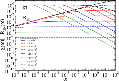
Figure 4: Relative response amplitude $|\chi(\omega)|$ (in units of $\chi_{0}$) and signal-to-noise ratio $R_{\rm SN}(\omega)$ (in units of $B/\tau_{r}$) on circular frequency (in units of $\tau_{r}^{-1}$) for $\alpha=0.5$ and different values of $\langle\tau\rangle$. Notice that both the frequency domain of quasi-static response and the maximal value of $R_{\rm SN}(\omega)$ shrink as $1/\langle\tau\rangle$ with increase of $\langle\tau\rangle$ (in units of $\tau_{r}$).

II.4 Aging correlation function

Nonstationary response exists, however, even in non-ergodic systems Barbi ; Sokolov06 ; H07 ; West ; Allegrini09 . To describe nonstationary response also in ergodic systems driven initially out of equilibrium and left to relax or age to the new equilibrium (e.g. after a temperature jump), one needs to find non-stationary or aging correlation function of the unperturbed system $\langle x(t_{a}+t)x(t_{a})\rangle$ which depends on the system age $t_{a}$. For the considered CTRW model, it can also be found straightforwardly following to the derivation given in Appendix. One can repeat it with another first-time survival probability $\Phi^{(0)}(t|t_{a})$ which depends on the age of system $t_{a}$ instead of $\Phi^{(0)}(t)$. This yields

$$\langle x(t_{a}+t)x(t_{a})\rangle_{0}=\langle\delta x^{2}\rangle_{0}\Phi^{(0)}(t|t_{a})+\langle x\rangle_{0}\langle x\rangle_{\rm st},$$ (28)

where averaging $\langle...\rangle_{0}$ is done over initial distribution $p_{j}(0)$ which generally is different from the stationary one, and $\langle\delta x^{2}\rangle_{0}:=\langle x^{2}\rangle_{0}-\langle x\rangle_{0}\langle x\rangle_{\rm st}$. The major problem is reduced to finding $\Phi^{(0)}(t|t_{a})$. The central role is played indeed by the first time survival probability, as already well-established Godreche ; BarkaiMargolin ; Allegrini05 ; West for symmetric two state process of the kind considered. It features also our fully decoupled CTRW model with arbitrary number of states. Aging $\Phi^{(0)}(t|t_{a})$ can be found from the exact relation similar to one discussed for forward recurrence-time in Refs. Cox ; Allegrini05 ,

$$\Phi^{(0)}(t|t_{a})= \Phi(t+t_{a})$$ (29)

$$+ \sum_{n=1}^{\infty}\int_{0}^{t_{a}}\psi_{n}(t_{a}-y)\Phi(t+y)dy,$$ (30)

where $\psi_{n}(t)$ is the probability density to have $n$ scattering events. It is the $n$-time convolution of the density $\psi(\tau)$, $\tilde{\psi}_{n}(s)=[\tilde{\psi}(s)]^{n}$ in the Laplace space. Indeed, let assume that our system was newly prepared at the time $-t_{a}$ in the past relative to the starting point of observations $t_{0}=0$. Then, the first term (29) is just the probability to stay from $-t_{a}$ until $t$ without any scattering event. However, $n$ such intermittent events can occur until any “unseen” time point $-y$ within the time interval $[-t_{a},0]$ in the past and then no events occur until $t$. Integrating over $y$ and summing over all possible $n$ yields the above exact result. From it, one can easily find the double Laplace transform $\tilde{\Phi}^{(0)}(s|u)$, where $s$ is Laplace-conjugated to $t$ and $u$ to $t_{a}$. Some algebra yields simple result

$$\tilde{\Phi}^{(0)}(s|u)=\frac{1}{u(s-u)}\left(1-\frac{\tilde{\Phi}(s)}{\tilde{\Phi}(u)}\right)\;.$$ (31)

The Laplace-transform of the fully aged $\Phi^{(0)}(t)=\lim_{t_{a}\to\infty}\Phi^{(0)}(t|t_{a})$, the first-time stationary survival probability, can be obtained now as $\tilde{\Phi}^{(0)}(s)=\lim_{u\to 0}u\tilde{\Phi}^{(0)}(s|u)$. For $\tilde{\Phi}(0)=\langle\tau\rangle\neq\infty$ this reproduces the well-known result in Eq. (8) and provides a very important consistency check. And for $\tilde{\Phi}(0)=\infty$, $\tilde{\Phi}^{(0)}(s)=1/s$, or $\Phi^{(0)}(t|\infty)=\Phi^{(0)}(t)=1$. This entails again the death of stationary response. In this case, nonstationary response to a periodic signal is dying to zero asymptotically, as found for a two-state nonergodic dynamics in Ref. Barbi . Ergodic systems with finite $\langle\tau\rangle$ will also exhibit aging response being prepared in a non-equilibrium state at some $-t_{a}\neq-\infty$ in the past, e.g. after a temperature jump. Their response but approaches non-zero stationary limiting value featuring new equilibrium state, which has been considered in this work. This is what normally seen in most aging experiments: response to a periodic signal gradually dies out and approaches a stationary non-zero limit Lunken .

Nonstationary aging response within the considered model will be studied in detail elsewhere. As an intelligent guess based on multi-state Markovian dynamics Marconi ; Cugliandolo ; Lippielo in the absence of stationary fluxes in unperturbed dynamics, the two-time inhomogeneous response function should read

$$\chi(t,t^{\prime})=\frac{H(t-t^{\prime})}{2k_{B}T}\Big{[}\frac{\partial}{\partial t^{\prime}}\langle\delta x(t)\delta x(t^{\prime})\rangle$$

$$-\frac{\partial}{\partial t}\langle\delta x(t)\delta x(t^{\prime})\rangle\Big{]}\;,$$ (32)

with $\langle\delta x(t)\delta x(t^{\prime})\rangle=\langle\delta x^{2}\rangle_{t^{\prime}}\Phi^{(0)}(t-t^{\prime}|t^{\prime})$, $T$ being the temperature after the temperature quench and

$$\langle\delta x(t)\rangle=\int_{t_{0}}^{t}\chi(t,t^{\prime})f(t^{\prime})dt^{\prime},$$ (33)

with external field starting to act at $t=t_{0}$. As to the survival probability $\Phi(t)$ incorrectly used instead of $\Phi^{(0)}(t)$ in most CTRW theories of stationary response in thermally equilibrium environments, it corresponds to $\Phi^{(0)}(t|t_{a})$ at zero age $t_{a}=0$, $\Phi(t)=\Phi^{(0)}(t|0)$, i.e. to the response of systems mostly deviating from thermal equilibrium, and not mostly close to it. Clearly, it does not describe even nonstationary zero-age response in aging systems.

III Discussion and Conclusions

In this work, we showed within a multistate renewal model that nonergodic systems featured by infinite mean waiting times cannot respond asymptotically to stationary signals. This questions a good part of the anomalous response theory based on such processes. A common fallacy in the corresponding literature consists in failure to find the correct stationary autocorrelation function which can be used as a phenomenological input in the fundamental microscopical theory of stationary linear response by Kubo and others. In this respect, our critique is similar to one by Tunaley Tunaley earlier. More important, we studied the way how the stationary response dies out with increasing mean waiting times in a model with one normal and one anomalous relaxation channel acting concurrently and in parallel. The normal channel defines the mean waiting time. This model reproduces approximately the Cole-Cole response in the limit where mean time is much less than the anomalous relaxation time defining the time of Cole-Cole response (about inverse frequency at the maximum of absorption line defined by ${\rm Im}[\hat{\chi}(\omega)]\propto\omega S(\omega)$). Paradoxically enough, such a response is more anomalous, with index $1-\alpha$, for less anomalous relaxation channels with index $\alpha$ closer to one. Then, the resulting stochastic process becomes closer to $1/f$ noise. This provides an elegant way to explain the origin of $1/f$ noise within ergodic dynamics featured by stationary response.

Absence of stationary response for nonergodic dynamics with infinite mean waiting times does not mean of course that the response is totally absent. It will be dying down to zero in the course of time as clarified earlier for two-state nonergodic dynamics Barbi ; West . However, it can be of primary importance for reacting on non-stationary signals only transiently present – a common situation in many biological applications Goychuk01 , or for other complex nonergodic input signals West . For example, response of neuronal systems to boring constant step signals should normally be damped out (a healthy reaction), and this is indeed the case as shown in several experiments Nature1 ; French ; Nature2 . This is a sign of complexity West . A theory of such dying nonstationary response within CTRW approach has been initiated in Refs. Barbi ; Allegrini09 ; West and we refer interesting readers to those works. They laid grounds for a continuing scientific exploration of the response of non-ergodic, non-stationary and aging systems which encompass also this author and readers. This fascinating scientific exploration is now at the very beginning. I am confident that it will attract ever more attention in the future.

Appendix A Calculation of autocorrelation function

Stationary function $\langle x(t)x(0)\rangle_{\rm st}$ can be found as $\langle x(t+t_{0})x(t_{0})\rangle_{\rm st}=\sum_{i,j}x_{i}x_{j}P^{(\rm st)}(i,t+t_{0};j,t_{0})$, where $P^{(\rm st)}(i,t+t_{0};j,t_{0})$ is two-time stationary probability density of the process $x(t)$ (joint probability). It depends only on the time difference of arguments and can be expressed through the corresponding stationary conditional probability density or propagator $\Pi^{(\rm st)}(i,t|j,0)$ as $P^{(\rm st)}(i,t+t_{0};j,t_{0})=\Pi^{(\rm st)}(i,t|j,0)p_{j}^{(\rm st)}(0)$, where $p_{j}^{(\rm st)}(0)$ is stationary single-time probability density. How to construct stationary propagator of such and similar CTRW processes is explained in detail in Refs. Goychuk04 ; GH05 . Along similar lines, we introduce the matrix of waiting time densities $\mathbf{\Psi}(\tau)$ which in the present case is expressed through the only one density $\psi(\tau)$. In components, $\Psi_{ij}(\tau)=\psi(\tau)\delta_{ij}$, where $\delta_{ij}$ is Kronecker symbol (unity matrix $\mathbf{I}$). Next, we introduce the transition matrix $\mathbf{T}$ with component $T_{ij}$ being the transition probability from the state $j$ to the state $i$ as a result of scattering event. Matrix of survival probabilities is $\mathbf{\Phi}(t)=\Phi(t)\delta_{ij}$. Moreover, we need the matrices of the first time densities, $\Psi_{ij}^{(0)}(\tau)=\psi^{(0)}(\tau)\delta_{ij}$ and the first time survival probabilities, $\Phi_{ij}^{(0)}(t)=\Phi^{(0)}(t)\delta_{ij}$, $\Phi^{(0)}(t)=\int_{t}^{\infty}\psi^{(0)}(t^{\prime})dt^{\prime}$. Stationary propagator is is easy to find in the Laplace-space, $\tilde{P}^{(\rm st)}(i,s|j,0)=\int_{0}^{\infty}P^{(\rm st)}(i,t|j,0)e^{-st}dt$ (tilde denotes the corresponding Laplace-transform for any function). Then, the conditional state probabilities to remain in the initial state are captured by $\tilde{\mathbf{\Phi}}^{(0)}(s)$. Contribution of the path with one scattering event is $\tilde{\mathbf{\Phi}}(s)\mathbf{T}\tilde{\mathbf{\Psi}}^{(0)}(s)$. Two scattering events contribute as $\tilde{\mathbf{\Phi}}(s)\mathbf{T}\tilde{\mathbf{\Psi}}(s)\mathbf{T}\tilde{\mathbf{\Psi}}^{(0)}(s)$, and so on. All in all,

$$\tilde{\mathbf{\Pi}}^{(\rm st)}(s)= \tilde{\mathbf{\Phi}}^{(0)}(s)$$

$$+\tilde{\mathbf{\Phi}}(s)\sum_{n=0}^{\infty}\left[\mathbf{T}\tilde{\mathbf{\Psi}}(s)\right]^{n}\mathbf{T}\tilde{\mathbf{\Psi}}^{(0)}(s)$$

$$=\tilde{\mathbf{\Phi}}^{(0)}(s)+\tilde{\mathbf{\Phi}}(s)\frac{1}{\mathbf{I}-\mathbf{T}\tilde{\mathbf{\Psi}}(s)}\mathbf{T}\tilde{\mathbf{\Psi}}^{(0)}(s).$$

This expression is quite general and valid for other models of $\mathbf{T},\tilde{\mathbf{\Phi}}(s),\tilde{\mathbf{\Psi}}(s)$, and $\tilde{\mathbf{\Phi}}^{(0)}(s),\tilde{\mathbf{\Psi}}^{(0)}(s)$. Further calculations are straightforward for the considered model, $T_{ij}=p_{i}$, $\sum_{i}p_{i}=1$. The first term in (A) contributes as $\langle x^{2}\rangle_{\rm st}\Phi^{(0)}(t)$ to the correlation function. The series also can be summed exactly by using that $(\mathbf{T}\mathbf{\Psi})_{ij}=p_{i}\psi$, or $\mathbf{T}\mathbf{\Psi}=\psi\mathbf{T}$, and $(\mathbf{T}\mathbf{\Psi})^{2}=\psi^{2}\mathbf{T}$ repeatedly, and standard relations between the densities and survival probabilities like $\tilde{\Phi}(s)=[1-\tilde{\psi}(s)]/s$. The series term contributes as $\langle x\rangle^{2}_{\rm st}\tilde{\psi}^{(0)}(s)/s$, and after some algebra we obtain the simple exact result

$$\langle x(t)x(0)\rangle_{\rm st}=\langle\delta x^{2}\rangle_{\rm st}\Phi^{(0)}(t)+\langle x\rangle_{\rm st}^{2},$$ (36)

with $\langle\delta x^{2}\rangle_{\rm st}=\langle x^{2}\rangle_{\rm st}-\langle x\rangle_{\rm st}^{2}$. This yields covariance (18) upon identifying stationary averages with thermal equilibrium averages. This result is valid for any number of states within the fully decoupled CTRW model.

The simplest stationary process of this kind is two-state semi-Markov process considered by Geisel et al. Geisel for velocity variable, as a statistical model for chaotic dynamics. It must be stressed that $\psi(\tau)$ is not the time probability density to stay in the corresponding state because at each scattering event the particle can remain in the same state. This is waiting time distribution between scattering events. This process differs from the alternating symmetric two-state process considered by Stratonovich, et al. Stratonovich ; GH03 . The last one alternates at each scattering event with the probability one, i.e. $T_{11}=T_{22}=0$, $T_{12}=T_{21}=1$. In such a case, $\psi(t)$ denoted for this model as

References

- (1) J. Klafter, S. C. Lim, and R. Metzler (eds.) Fractional Dynamics: Recent Advances (World Scientific, Singapore, 2011).
- (2) M. F. Shlesinger, J. Stat. Phys 10 (1974) 421.
- (3) H. Scher and E. M. Montroll, Phys. Rev. B 12 (1975) 2455.
- (4) B. D. Hughes, Random walks and Random Environments, Vols. 1,2 (Clarendon Press, Oxford, 1995).
- (5) R. Metzler and J. Klafter, Phys. Rep. 339, 1 (2000).
- (6) R. Kubo, Rep. Prog. Phys. 29 (1966) 255.
- (7) W. T. Coffey, Y. P. Kalmykov, The Langevin Equation: With Applications to Stochastic Problems in Physics, Chemistry and Electrical Engineering, 3d ed. (World Scientific, Singapore, 2012).
- (8) U. Weiss, Quantum Dissipative Systems, 2nd ed. (World Scientific, Singapore, 1999).
- (9) I. Goychuk, Adv. Chem. Phys. 150 (2012) 187.
- (10) R. Balescu, Statistical dynamics: matter out of equilibrium (Imperial College Press, London, 1997).
- (11) E. Barkai and R. J. Silbey, J. Phys. Chem. B104 (2000) 3866.
- (12) J.-P. Bouchaud and A. Georges, Phys. Rep. 195 (1990)127.
- (13) S. Havlin and D. Ben-Avraham, Adv. Phys. 51 (2002) 187.
- (14) K. S. Cole and R. H. Cole, J. Chem. Phys. 9 (1941) 341.
- (15) P. Lunkenheimer, U. Schneider, R. Brand, and A. Loid, Contem. Phys. 41 (2000) 15.
- (16) H. Oukris and N. E. Israeloff, Nature Phys. 6 (2009) 135.
- (17) P. Lunkenheimer, R. Wehn, U. Schneider, and A. Loidl, Phys. Rev. Lett. 95 (2005) 055702.
- (18) A. Papoulis, Probability, Random Variables, and Stochastic Processes (McGraw-Hill Book Company, New York, 1991), pp. 430-432.
- (19) R. Zwanzig, Nonequilibrium Statistical Mechanics (Oxford University Press, Oxford, 2001).
- (20) U. M. B. Marconi, A. Puglisi, L. Rondoni, and A. Vulpiani, Phys. Rep. 461 (2008) 111.
- (21) D. Villamaina, A. Sarracino, G. Gradenigo, A. Puglisi, and A. Vulpiani, J. Stat. Mech. Theor. Exp. (2011) L01002.
- (22) G. Gradenigo, A. Sarracino, D. Villamaina, and A. Vulpiani, J. Stat. Mech. Theor. Exp. (2012) L06001.
- (23) L. F. Cugliandolo, J. Kurchan, and G. Parisi, J. Phys. I 4 (1994) 1641.
- (24) E. Lippiello, F. Corberi, and M. Zannetti, Phys. Rev. E 71 (2005) 036104.
- (25) R. Gorenflo, F. Mainardi, in: Fractals and Fractional Calculus in Continuum Mechanics edited by A. Carpinteri, F. Mainardi (Springer, Wien, 1997), pp. 223-276.
- (26) J. K. E. Tunaley, Phys. Rev. Lett. 33 (1974) 1037.
- (27) I. Goychuk and P. Hänggi, Phys. Rev. Lett. 91 (2003) 070601; Phys. Rev. E 69 (2004) 021104.
- (28) I. Goychuk and P. Hänggi, Adv. Phys. 54 (2005) 525.
- (29) D. E. Cox, Renewal Theory (Methuen,London, 1962).
- (30) I. Goychuk, Phys. Rev. E 76 (2007) 040102(R).
- (31) F. Barbi, M. Bologna, and P. Grigolini, Phys. Rev. Lett. 95 (2005) 220601.
- (32) I. M. Sokolov and J. Klafter, Phys. Rev. Lett. 97 (2006) 140602.
- (33) E. Heinsalu, M. Patriarca, I. Goychuk, and P. Hänggi, Phys. Rev. Lett. 99 (2007) 120602; Phys. Rev. E 79 (2009) 041137.
- (34) B. J. West, E. L. Geneston, and P. Grigolini, Phys. Rep. 468 (2008) 1.
- (35) P. Allegrini, et al. Phys. Rev. Lett. 103 (2009) 030602.
- (36) G. Margolin and E. Barkai, J. Chem. Phys. 121 (2004) 1566.
- (37) A. I. Saichev and S. G. Utkin, JETP 99 (2004) 443; A. Stanislavsky, K. Weron, and A. Weron, Phys. Rev. E 78 (2008) 051106.
- (38) I. Goychuk, Phys. Rev. E 86 (2012) 021113.
- (39) V. M. Kenkre, E. W. Montroll, and M. F. Shlesinger, J. Stat. Phys. 9 (1973) 45.
- (40) I. Goychuk, Phys. Rev. E 70 (2004) 016109.
- (41) I. M. Sokolov and J. Klafter, Chaos 15 (2005) 026103; A. V. Chechkin, V. Yu. Gonchar, R. Gorenflo, N. Korabel, and I. M. Sokolov, Phys. Rev. E 78 (2008) 021111.
- (42) M. B. Weismann, Rev. Mod. Phys. 60 (1988) 537.
- (43) L. Gammaitoni, P. Hänggi, P. Jung, and F. Marchesoni, Rev. Mod. Phys. 70 (1998) 223.
- (44) C. Godreche and J. M. Luck, J. Stat. Phys. 104 (2001) 489.
- (45) P. Allegrini, et al. Phys. Rev. E 71 (2005) 066109.
- (46) I. Goychuk, Phys. Rev. E 64 (2001) 021909; I. Goychuk and P. Hänggi, Eur. Phys. J. B 69 (2009) 29.
- (47) K. M. Chapman and R. S. Smith, Nature (London) 197 (1963) 699.
- (48) A. S. French, Biophys. J. 46 (1984) 285.
- (49) B. N. Lundstrom, M. H. Higgs, W. J. Spain, and A. L. Fairhall, Nat. Neurosci. 11 (2008) 1335.
- (50) T. Geisel, A. Zacherl, and G. Radons, Z. Phys. B 71 (1988) 117.
- (51) R. L. Stratonovich, Topics in the Theory of Random Noise vol. 1 (Gordon and Breach, New York, 1963), p. 176.