Mobility transition in a dynamic environment
Abstract
Depending on how the dynamical activity of a particle in a random environment is influenced by an external field , its differential mobility at intermediate can turn negative. We discuss the case where for slowly changing random environment the driven particle shows negative differential mobility while that mobility turns positive for faster environment changes. We illustrate this transition using a 2D-lattice Lorentz model where a particle moves in a background of simple exclusion walkers. The effective escape rate of the particle (or minus its collision frequency) which is essential for its mobility-behavior depends both on and on the kinetic rate of the exclusion walkers. Large , i.e., fast obstacle motion, amounts to merely rescaling the particle’s free motion with the obstacle density, while slow obstacle dynamics results in particle motion that is more singularly related to its free motion and preserves the negative differential mobility already seen at . In more general terms that we also illustrate using one-dimensional random walkers, the mobility transition is between the time-scales of the quasi-stationary regime and that of the fluid limit.
pacs:
74.40.Gh, 05.70.Ln, 05.40.-a1 Introduction
The differential mobility of a colloid in a medium measures how for a given external field its velocity increases with changing . A well–known implication of the fluctuation–dissipation theorem for an equilibrium environment at temperature is the Sutherland-Einstein relation between the diffusion constant at zero field and the mobility , [1]. Going to higher -values, this equality fails [2] and even more interestingly, it easily happens that implying that pushing harder slows down the particle [3, 4]. A possible unifying framework for understanding these negative differential mobilities (and other conductivities [5]) has been found in the study of nonequilibrium response [6]. There enters the dynamical activity which is a measure of time–symmetric currents and expresses a “nervosity” of the particle during its motion. The point is that the nonequilibrium contribution to the response modifies the Sutherland–Einstein (or more generally, the Kubo) formula by subtracting from the time–correlation function between the velocity of the particle and its differential dynamical activity, which can be large. We have called it the frenetic contribution [7] to contrast it with the entropic contribution which makes the standard Green–Kubo or Helfand term, [8, 9, 10].
The present paper adds an extra parameter in the study of the differential mobility , denoting in general by an inverse time-scale or the rate at which constituents of the environment are themselves moving. We consider here single particles moving in a bath of obstacles. This is an example of the more general study of random walks in a dynamic random environment; see e.g. [11, 12] in the mathematics literature. Parameters like can refer to the changing architecture or geometry of the environment, or they can effectively parametrize the dynamics of the particle. In all cases here we assume that the dynamics of the environment is itself undriven for fixed particle position. Specific examples follow in the next sections. For broader physics background on the models and for previous work we also refer to [13, 14, 15, 16].
The scenario is always that for some range of , where indicates a static (or quenched) random environment. The case is however a singular limit. Our main study and observation is that the negativity
is stable for after which, for , the differential mobility is positive for all fields . In other words, there is a finite threshold field (only) for . The critical value first of all marks the regime of quenched static random environment and the regime of annealed random environment. Indeed, taking the time-scale at which the driven particle moves to be of order one for all values of the field , we have that corresponds to large time-separation under which the particle moves in an averaged–out environment where . That can be called the fluid limit. Secondly, the regime is quasi-stationary for the particle, where the relaxation time for the particle dynamics is still much smaller than the time-scale for the environment. In other words, negative response is expected to hold when for . If , it suffices that which implies that is very small when grows fast with the field .
The plan of the paper is as follows. We start in the next section with the general question in the context of integrating out a dynamic environment. Section 3 is devoted to a computational and numerical analysis of the lattice Lorentz model with moving obstacles as random dynamic environment. We describe the regime of negative differential mobility where is the driving field on the particle and is the rate at which the individual obstacles move. Section 4 is devoted to a number of toy-models of walkers in quasi-one dimensional architectures that enable easier access for understanding the mobility transition.
2 General question
A tagged degree of freedom (called, particle position) is subject to a constant external driving and moves in a dynamical environment (called, obstacles). We do not assume that the coupling is “weak,” or that the particle is “small” or that its motion is “slow” with respect to the obstacles. Particle and obstacles are coupled and are in weak contact with an equilibrium bath at a fixed inverse temperature that we set to one. The obstacles are undriven and the whole process is reversible at . For fixed particle position the obstacles can be considered to be an equilibrium fluid specified by some density and inverse temperature . Calling a measure for the time-scale separation between obstacle and particle dynamics, we have corresponding to that equilibrium fluid limit. On the other hand, for the particle sees a quasi–static random environment.
We consider the regime where the motion of the undriven particle ( but arbitrary ) is asymptotically diffusive with a linear response regime in satisfying the Kubo or Sutherland-Einstein relation. The general question is to understand the dependence of the particle velocity versus field also for intermediate and large as a function of . Selecting the direction of that field as the one–dimensional space for the particle’s position, one version of the question boils down to understanding the effective particle’s motion under coarse–graining, i.e., after integrating out the environment. To characterize that effectively one–dimensional motion and for simplicity assuming a Markovian random walk we essentially need to know the effective rate of moving forward () and that of moving backward ().
A more physical parametrization is contained in two types of information:
(1) Because of the undriven character of the environment, we expect that the effective biasing field on the particle is essentially still given by . From the hypothesis of local detailed balance [17] we would then get
| (1) |
where it cannot be excluded entirely that the effective temperature because of possible entropy fluxes between particle and obstacles at some different effective temperature depending on and . If however the obstacle density is low or is large, we expect to very good approximation.
(2) The effective escape rate
| (2) |
measures the dynamical activity of the particle in terms of the time–symmetric current along the direction of the field.
Taking that picture of the one–dimensional walker seriously and combining (1) with (2) we would obtain a speed of the particle in the direction of the field specified as
| (3) |
The primary question addressed here is whether it is possible to have a non-monotonic dependence of on the field or in other other words, whether this system shows negative differential mobility and for what For the linear behavior around equation (3) gives or . For intermediate and large in (3) the variation of the speed with crucially depends on how behaves with for a given . In particular, taking now , if decreases fast enough with the driving field , then it is possible to have such a scenario. As ultimately refers to the activity of the particle, we are led to the question whether the particle gets more or gets less ‘trapped’ by increasing . In the next section we focus on a specific model system, namely lattice Lorentz gas with moving obstacles, to investigate these questions.
3 Model
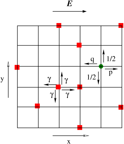
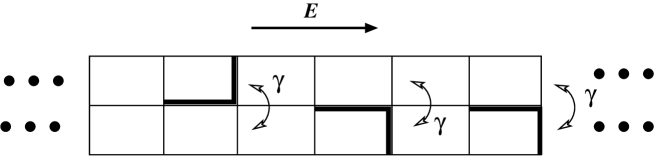
Let us consider particles distributed on a 2D square lattice of size We assume periodic boundary conditions and the density does not evolve in time. These particles, referred to as the ‘obstacles’ or ‘sea particles,’ perform a symmetric simple exclusion process with rate . There is another ‘charged’ or ‘probe’ particle in the system which is driven by an ‘electric’ field pointing in the direction. Consequently this charged particle performs a biased random walk in the -direction — it moves to the right (left) with rate while the motion along the -direction is symmetric — the rates of moving up and moving down are equal to (see Fig. 1). We assume local detailed balance [17] so that The charged particle interacts with the sea particles via exclusion — it can move only when the target site is empty; the sea particles act as ‘obstacles’ for the charged one. This model can thus be considered as a lattice Lorentz gas with moving obstacles, [18].
A discrete time version of the model is studied in [13]; here we work in continuous time where the jumps have rates which follow the condition of local detailed balance [17]. The local detailed balance condition does not specify the rates completely however; we choose
| (4) |
so that in the absence of obstacles the escape rate in the horizontal direction is In that way, we do not impose by hand a specific change in escape rate for varying field at zero obstacle density (free motion). Note that for large .
To numerically simulate this system, we use a random sequential updating scheme. First a site is selected randomly - if it is occupied by the probe particle or a sea particle then it attempts to jump to one of the four neighbouring sites with corresponding rates, the attempt being successful only when the target site is empty. On the other hand if the selected site is vacant then nothing is done. In this scheme each update, whether successful or not, corresponds to an increase in time
Let denote the net number of steps per unit time that the charged particle makes in the -direction. An expression for the average speed can be obtained from the dynamical updating rules. Let us denote the instantaneous position of the charged particle by Also let denote the occupation number for the sea particles, , depending on whether site is occupied by a sea particle or not. Then, the dynamics gives
| (5) |
The expectation measures the probability (or fraction of time) that the right neighbouring site of the charged particle is occupied, and similarly for . Or, with denoting the total time in during which there is an obstacle to the right (left) neighbouring site of the charged particle, we have under stationary conditions that
| (6) | |||||
| (7) |
where we identify,
That is the speed of a biased one–dimensional random walker with effective rates and we are exactly realizing the spirit of formula (3). Following these ideas we then expect negative differential mobility when the effective escape rate decreases sufficiently fast as a function of .
Static Obstacles:
The case corresponds to the driven lattice Lorentz gas and is known to show negative response irrespective of the choice of [6, 16, 19]. The study of this system was started in the context of diffusion in random media with focus on the phase transition to a zero–current regime [19, 20, 21, 22]. Here we concentrate on the origin of the non–monotonicity of the velocity as a function of the field to understand the stability of the phenomenon for .
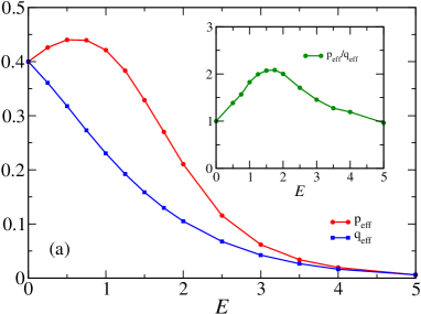
The effective rates and as defined in (7), are plotted as a function of the field in Fig. 2(a). The effective bias measured from the ratio is shown in the inset. The non–monotonic nature of this curve indicates a strong violation of the local detailed balance in the steady state. Fig. 2(b) shows a plot of the sum of these quantities (dark circles) which is a measure of the dynamical activity. The inset suggests that this effective escape rate is exponentially decaying for large field
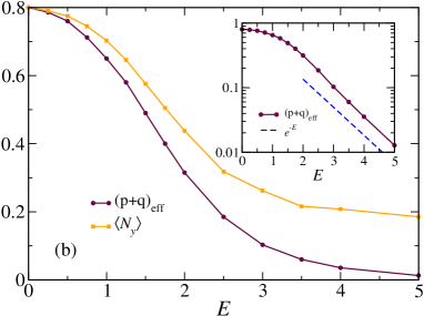
As the stationary velocity is given by (3), and both the factors and are decreasing for large , the differential mobility becomes strongly negative. Fig. 3 (a) shows the stationary speed as a function of the field it shows a strong negative differential mobility for
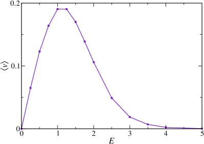
Interestingly, the activity in the -direction as quantified by the average number of vertical jumps per unit time is also decreasing with the field; see the upper curve (light orange squares) in Fig. 2(b). In contrast with the free motion in 2D the motion in the - and in the -directions are no longer independent.
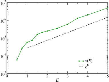
It should be emphasized however that the situation is a somewhat singular limit. Various correlation functions do not reach a stationary value (at least within feasible computational time) for large fields. The relaxation time , defined as the time required to reach a stationary velocity, increases exponentially with the field Fig. 3(b) appears to verify at least for large Secondly and related, the stationary distribution of the charged particle depends on the obstacle configurations for . All the simulations that we present here are thus averaged over many (from about 600 for large fields to 1000 for small fields) obstacle configurations, with 100 trajectories for each configurations. The lattice considered is a square of size with periodic boundary conditions in both directions.
Moving obstacles :
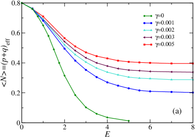
The non–zero presents a dynamic environment for the charged particle which leads to a unique stationary behaviour and the charged particle’s position is uniformly distributed over the lattice. Nevertheless, one can expect a negative differential response
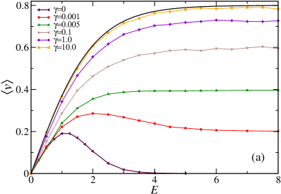
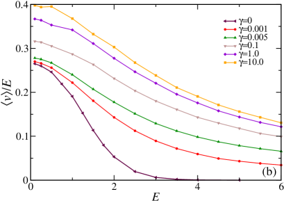
for ‘reasonably’ small , i.e., when the time scale associated to the charged particle is small compared to the sea particles. This picture is verified in Fig. 4(a) where we have plotted the dependence of the average speed on the external field for different values of ranging from to for The negative response is seen for very small values of like The average speed becomes monotone increasing in for (dark green triangles in Fig. 4(a)). As is increased further the average speed approaches (solid black line) as is expected in the fluid limit. Instead of looking at the differential mobility, one can also consider the absolute mobility, defined as the ratio of average velocity and the applied field shown in Fig. 4(b). The initial constant region
corresponds to the linear response (Kubo) regime. Clearly, the presence of the transition in differential mobility is not directly reflected from the behaviour of ordinary mobility. The results remain qualitatively similar for other values of the density ; the absolute value of the current decreases of course as one goes to higher density. One difference with is the limit for the average speed, saturating
at a non-zero -dependent value whenever (see (15) below).
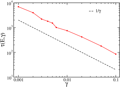
The relaxation time of the charged particle now depends on both and and we expect for a fixed and large as can be verified from Fig. 5. On the other hand, the relaxation time for fixed increases exponentially with the field (not shown).
Similar to the case we measure the effective dynamical activity and effective bias from the stationary values of and Fig. 6(a) shows the dependence on of that effective escape rate for different small values of for the sake of comparison we have added the escape rates for the case too. Clearly the effective escape rates behave similarly in all these cases, decreasing in . However, only for small the decay is fast enough to result in a non-monotonic velocity implying negative differential mobility. The corresponding effective biasing field behaves as as shown in Fig. 6(b) thus maintaining the local detailed balance. In fact the effective temperature defined in (1) remains equal to at least for large field
3.1 Response : Differential Mobility
The differential mobility is the linear response coefficient of the speed to the perturbation
The corresponding response formula is most conveniently derived using the path-integration formalism of A. We give here the result for the choice (4).
For a general path-observable of the system over a time-interval we find
| (8) |
where denote connected correlation functions. Here, denotes the total number of jumps (right or left) made by the charged particle in time along the -direction; is the total current and the speed is The observables and are the dwelling times as defined through (7) in the previous section. Choosing in (8) gives

Note that the escape rate of the walker defined through (2) equals as follows from comparing (7) with (3.1). Following the writing of (3), we then get the exact identity
| (10) |
where
with Fig. 6(b) showing indeed that for large . It is therefore the decrease of with large that decides the negative differential conductivity.
Continuing with (8) the response of the average speed is the differential mobility
| (11) |
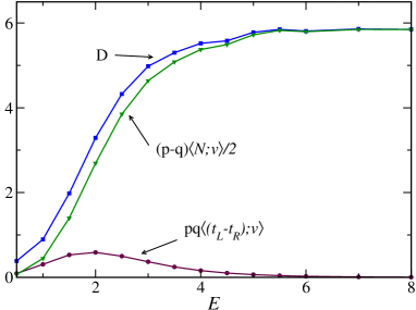
The first term is nothing but the diffusion constant for the charged particle which has its origin in the entropic contribution to the response. The other so called frenetic terms are truly nonequilibrium input and come from the time–symmetric part of the action; see A. We emphasize that this response relation considers only the mobility of the charged particle to the change in field and holds true for any value of including zero. When and for no matter what the mobility equals the diffusion constant (Sutherland–Einstein relation). The effects of and are implicitly present in the expectations because the whole dynamical process depends on and . The different terms appearing in the response formula (11) are plotted against in Fig.7 for for which the negative response is most prominent. Note that the diffusion and the last term in (11 ) approach each other for large field so that the response becomes almost equal to :
In the light of that formula, negativity of around is then due to the strong positivity of the correlation between the difference in dwelling times near obstacles (left versus right) and the current . The picture that emerges is that for large and small the charged particle traces a path keeping to the immediate right of the obstacles while for large and large the charge waits some time left of the obstacles. It thus resembles the strategy of a pedestrian who hurries to cross a square with randomly moving walkers; when these move fast, the pedestrian can afford to keep going straight and to wait a bit in front of each walker when blocked — when the walkers move slow, the pedestrian will prefer to slalom around them.
It is also possible to express the current in nonlinear response around . The same type of computations are involved as in the above; see again A. We then get with
| (12) |
in terms of expectations at and where the last term equals the fourth cumulant of . Presence of a negative differential response would basically mean that is positive. Measuring the positivity of from numerical simulations for small turns out however to be very difficult. That appears compatible with difficulties in computing (super-)Burnett coefficients, [23]. In general for characterizing a nonequilibrium regime, linear response around a stationary process possibly far from equilibrium is more useful than nonlinear response in expansion around equilibrium.
3.2 Heuristics
As mentioned in the introduction there are two regimes, a quasi–stationary regime where for small the obstacles move much slower than the charged particle and a similar behaviour to is seen, and a fluid regime for large where the charged particle moves as in an equilibrium fluid with background density .
The fluid regime is characterized by where the effective parameters become as indeed recovered numerically.
The quasi–static regime is specified by the relaxation time of the charged particle being much smaller with respect to . There a similar behavior as for is observed, including the negative differential mobility . If, with , then . Being optimistic we could put at first for small to estimate the critical from equating
Since the numerics show and , we would get while the simulations give which is off by one order of magnitude. The reason is probably that for the relevant values of and the relaxation time is still one order of magnitude smaller than .
There is thus a critical with for the existence of a finite with negative differential mobility for a range of , while for all if . In what follows we provide exact results for some analogous toy models to further support the above numerical evidence and this scenario in particular.
4 Simplified random walker models
An exact solution of the Lorentz model in a dynamic environment is of course very difficult to obtain when the time-scales of particle vs. environment do not diverge, . Yet the very similar phenomenon of mobility transition can be exactly obtained for a number of much simpler quasi–one–dimensional random walkers.
To start we can consider a biased random walker on two lanes, see Fig. 8, quite similar to the model in [3]. Motion in the horizontal direction is biased as in (4) for external field and the vertical transitions (between the lanes) happen at rate if there is no wall (thick horizontal line in Fig. 8). The vertical wall can either stand in the upper or in the lower lane blocking (closed) or unblocking (open) the horizontal transitions. To keep the analogue with the Lorentz model of above, we imagine a rate of transition for that wall (obstacle) moving up and down.

For we have a static environment and an exact solution can be easily obtained for any specific choice of obstacle configuration. For example, when all the vertically oriented obstacles are in the lower lane then the average speed is (see also [3, 6])
| (13) |
with a regime for the field with negative differential mobility. More precisely and in the notation of the previous sections,
At the other extreme, for (fluid limit) we obtain a monotonically increasing current Here, as in the Lorentz model with moving obstacles, there is a transition for a region of external fields where the differential mobility starts from being negative to become positive as increases; see Fig. 9. The threshold which separates the two regimes is estimated to be

This model can still be simplified further without any essential changes. We skip some steps in the simplification to arrive at a truly one–dimensional lattice as in Fig. 10.
All jumps towards the right occur with rate This includes jumps and in the forward direction. The rate for the jump in the corresponding backward directions is The vertical jump rate, i.e., between states 2 and 3 is symmetric and is denoted by
In the stationary state, the average current and differential mobility can be calculated explicitly. Following the choice (4) where the steady state probabilities of being in states and are
with The average current per unit time is then given by,
| (14) | |||||
| (15) |
For we find which vanishes for large For non–zero the average speed saturates to for
The plot in Fig. 11(a) shows exactly the same qualitative behaviour as for the driven Lorentz model in the previous section, compare with Fig. 4(a). It shows a transition in the sign of the differential mobility from negative for small (quasi-static regime) and sufficiently large, to being always positive in the fluid limit (large ). Note also that and can be computed from putting : the solution is
| (16) |


Fig. 11(b) shows a plot of rapidly increasing with and diverging at the critical .
5 Summary
We have studied linear response of a single particle under nonequilibrium driving in contact with a randomly evolving environment, parametrized by rate . We have shown that in the quasi–stationary regime, when the environment is slow enough, the differential mobility of the particle can become negative for large driving. On the other hand, for fast relaxing environment the system reaches a fluid limit with positive differential mobility for all values of the driving field. Thus one can expect a transition at a finite from ‘negative mobility’ to ‘positive mobility.’ Numerical evidence of this transition is provided with the example of the 2-dimensional Lorentz gas with moving obstacles. We have also illustrated this transition with a number of exactly solvable toy models.
Appendix A From path–integration to response
For various computations of response it is useful to apply a path-formalism [24, 7]. The starting point is the dynamical ensemble giving the probability distribution over all possible paths in configuration space over times , formally
where we compare the path-probabilities in an external field (left-hand side) with respect to the ensemble at zero-external field (in right-hand side). The action , function of the path over time interval , is for the driven lattice Lorentz model of Section 3 given by
| (17) |
where we have ignored field -independent terms ( depend on ). The response is governed by the derivative , since
| (18) | |||||
| (19) |
for a general path-observable on (not depending on ). Doing as (19) we get from (17) that
from which (8) follows when plugging in (4) (and leaving out the subscript ).
For further interpretations it is useful to make the decomposition where is (twice) the time–symmetric component and is antisymmetric under time–reversal. These are called the entropic () and the frenetic () components of the action and for Section 3 they equal, respectively,
| (20) | |||||
| (21) | |||||
| (22) |
These are again path–observables but they depend on the field ; we recognize as the path–dependent entropy production (linear in ) and as a measure of dynamical activity (nonlinear in ); recall that is the total number of jumps along the axis while is the net number in the positive direction.
For the nonlinear response around detailed balance () we proceed similarly. Taking to be the current in (19) we derive
| (23) |
where the primes denote derivatives. Inserting here with (22), we get at
| (24) |
The second term cancels as is symmetric under time–reversal whereas is antisymmetric. Similarly,
| (25) |
Each of the terms vanishes individually from symmetry considerations — the first three from time reversal symmetry and the last one from reflection (left-right) symmetry.
The third derivative in (23) is also calculated using (22)
which can be expressed as sums of cumulants and covariances:
| (27) |
That yields the expansion (12) to third order in .
References
- [1] A. Einstein, Annalen der Physik 17, 549 (1905).
- [2] M. Baiesi, C. Maes and B. Wynants, Proc. Royal Soc. A 467, 2792 (2011).
- [3] R.K.P. Zia, E. L. Præstgaard, and O.G. Mouritsen, Am. J. Phys. 70, 384 (2002).
- [4] S. Safaverdi, Transport and diffusion in nonequilibrium Langevin systems, Ph.D. thesis at KU Leuven, December 2013.
- [5] B. Li, L. Wang, G. Casati, Appl. Phys. Lett. 88, 143501 (2006).
- [6] P. Baerts, U. Basu, C. Maes, and S. Safaverdi, Phys. Rev. E 88, 052109 (2013).
- [7] M. Baiesi, C. Maes and B. Wynants, Phys. Rev. Lett. 103, 010602 (2009).
- [8] M. S. Green, J. Chem. Phys 22, 398 (1954).
- [9] R. Kubo, J. Phys. Soc. Jpn. 12, 570 (1957).
- [10] E. Helfand, Phys. Rev. 119, 1 (1960).
- [11] L. Avena, R. dos Santos, F. Völlering, arXiv:1102.1075.
- [12] L. Avena, F. den Hollander, F. Redig, Markov Proc. Relat. Fields 16, 139 (2010).
- [13] O. Bénichou, P. Illien, C. Mejía-Monasterio, and G. Oshanin, J. Stat. Mech. P05008 (2013).
- [14] O. Bénichou, A. M. Cazabat, J. De Coninck, M. Moreau, and G. Oshanin, Phys. Rev. B 63, 235413 (2001).
- [15] O. Bénichou, and G. Oshanin, Phys. Rev. E 66, 031101 (2002).
- [16] S. Leitmann, T. Franosch, Phys. Rev. Lett. 111, 190603 (2013).
- [17] S. Katz, J. Lebowitz, H. Spohn, J. Stat. Phys., 34, 497 (1984).
- [18] H. A. Lorentz, Proc. R. Acad. Sci. Amsterdam 7, 438 (1905).
- [19] D. Dhar, J. Phys. A: Math. Gen. 17, L257 (1984).
- [20] M. Barma and D. Dhar, J. Phys. C 16, 1451 (1983).
- [21] D. Dhar, D. Stauffer, Int. J. Mod. Phys. C 9, 349 (1998).
- [22] R. B. Pandey, Phys.Rev. B 30, 489 (1984).
- [23] J. M. J. van Leeuwen and A. Weijland,Physica 36, 457 (1967).
- [24] M. Baiesi, C. Maes and B. Wynants, J. Stat. Phys. 137, 1094 (2009).