Damping operators for the BBM equation

Long-time behavior of solutions of a BBM equation with generalized damping

Abstract. We study the long-time behavior of the solution of a damped BBM equation $u_{t}+u_{x}-u_{xxt}+uu_{x}+\mathscr{L}_{\gamma}(u)=0$. The proposed dampings $\mathscr{L}_{\gamma}$ generalize standards ones, as parabolic ($\mathscr{L}_{\gamma}(u)=-\Delta u$) or weak damping ($\mathscr{L}_{\gamma}(u)=\gamma u$) and allows us to consider a greater range. After establish the local well-posedness in the energy space, we investigate some numerical properties.

Keywords. BBM equation, dispersion, dissipation.

MS Codes. 35B40, 35Q53, 76B03, 76B15.

1 Introduction

The one-way propagation of small amplitude, long wavelength, gravity waves in shallow water can be described by the Korteweg-de Vries equation (KdV) [13]

$$u_{t}+u_{x}+u_{xxx}+uu_{x}=0.$$

or its regularized version, the Benjamin-Bona-Mahony (BBM) equation

$$u_{t}+u_{x}-u_{xxt}+uu_{x}=0.$$

Many works related to the damped KdV equation can be found in the literature ([2, 4, 5, 6, 8, 9, 10, 11, 14, 16, 17, 15] and references therein). These account for a wide variety of different results, such as regularizing effect of the damping, asymptotic behavior, existence of attractor or numerical computations. Few literatures are concerned the damped BBM equation [12, 18]. This paper consists in establishing theoretical and numerical results for the solution of a generalized damped BBM equation.

We introduce the following equation, called dBBM, for $x\in\mathbb{T}(0,L)$, $L>0$ and $t\in\mathbb{R}$

$$u_{t}+u_{x}-u_{xxt}+uu_{x}+\mathscr{L}_{\gamma}(u)=0,$$

where the operator $\mathscr{L}_{\gamma}$ is defined by its Fourier symbol

$$\widehat{\mathscr{L}_{\gamma}(u)}(k):=\gamma_{k}\hat{u}_{k}.$$

Here $\hat{u}_{k}$ is the $k-$th Fourier coefficient of $u$ and $(\gamma_{k})_{k\in\mathbb{Z}}$ are positive real numbers chosen such that

$$\int_{\mathbb{T}}u(x)\mathscr{L}_{\gamma}(u)d\mu(x)=\sum_{k\in\mathbb{Z}}\gamma_{k}|\hat{u}_{k}|^{2}\geq 0.$$

Standard dampings are included choosing $\gamma_{k}=k^{2}$ as parabolic damping or $\gamma_{k}=\gamma$ as weak damping. The proposed sequence $(\gamma_{k})_{k\in\mathbb{Z}}$ allows us to consider a greater range of damping. In particular, one may wonder if it is necessary to absorb all frequencies of a long wavelength gravity wave like the solution of KdV or BBM. To obtain this kind of results, we can consider sequences $\gamma_{k}\rightarrow 0$ when $|k|\rightarrow+\infty$ or even $\gamma_{k}=0$ for large $|k|$.

In comparison with the standard BBM equation for which the $H^{1}-$norm is preserved, we notice that the $H^{1}$-norm decreases for the solution $u$ of the damped equation dBBM. More precisely, we have for all time $t\in\mathbb{R}$

$$\frac{d}{dt}||u(t)||_{H^{1}}^{2}=-|u(t)|_{\gamma}^{2}\leq 0,$$

and the natural space to study the well-posedness is the space $H_{\gamma}(\mathbb{T})$, defined as

$$H_{\gamma}(\mathbb{T}):=\left\{u\in L^{2}(\mathbb{T});\sum_{k\in\mathbb{Z}}\gamma_{k}|\hat{u}_{k}|^{2}<+\infty\right\},$$

equipped with the norm

$$|u|_{\gamma}:=\sqrt{\sum_{k\in\mathbb{Z}}\gamma_{k}|\hat{u}_{k}|^{2}}.$$

In order to simplify the writings, $k$ can denote either an integer as an index, or the value $\frac{2\pi k}{L}$. When there is no ambiguity, we denote $C$ the different constants appearing in the following results.

The paper is organised as follows. We establish in Section 2 the local well-posedness of the dBBM equation. We prove some important estimates about the space $H_{\gamma}(\mathbb{T})$. Some qualitative properties of the solution are also given. In Section 3, numerical schemes are presented to solve the damped equation and to preserve the qualitative properties of the continuous solution. Section 4 deals with the numerical results. In particular, we manage to build a family of dampings weaker than the standard ones. These, for example taking $\lim_{|k|\to+\infty}\gamma_{k}=$ 0, yet provide dampen solutions.

2 Analysis of the problem

After studying the space $H_{\gamma}(\mathbb{T})$, we establish the well-posedness of the Cauchy problem associated with the dBBM equation.

2.1 Proper energy space $H_{\gamma}(\mathbb{T})$

Here we take $\gamma_{k}>0,\ \forall k\in\mathbb{Z}$. We first state some properties of injection.

Proposition 2.1.

Assume that $\sum\limits_{k\in\mathbb{Z}}\frac{1}{\gamma_{k}}<+\infty$. Then there exists a constant $C>0$ such that

$$\|u\|_{\infty}\leq C|u|_{\gamma}.$$

The injection $H_{\gamma}(\mathbb{T})\hookrightarrow L^{\infty}(\mathbb{T})$ is continuous.

Proof.

Let $u\in H_{\gamma}(\mathbb{T})$. We notice that

$$u(x)=\sum\limits_{k\in\mathbb{Z}}\hat{u}(k)e^{ikx}.$$

Then

$$|u(x)|\leq\sum\limits_{k\in\mathbb{Z}}|\hat{u}(k)|=\sum\limits_{k\in\mathbb{Z}}\frac{1}{\sqrt{\gamma_{k}}}\sqrt{\gamma_{k}}|\hat{u}(k)|.$$

We assumed that $\gamma_{k}>0$. Hence, the Cauchy-Schwarz inequality implies for all $x\in\mathbb{T}$ :

$$|u(x)|\leq\left(\sum\limits_{k\in\mathbb{Z}}\frac{1}{\gamma_{k}}\right)^{\frac{1}{2}}\left(\sum\limits_{k\in\mathbb{Z}}\gamma_{k}|\hat{u}(k)|^{2}\right)^{\frac{1}{2}}=\left(\sum\limits_{k\in\mathbb{Z}}\frac{1}{\gamma_{k}}\right)^{\frac{1}{2}}\left|u\right|_{\gamma}.$$

This completes the proof. ∎

Remark 2.2.

The above result is also a condition to have $\|\hat{u}\|_{l^{1}}\leq C|u|_{\gamma}$.

Proposition 2.3.

We assume that for all $k\in\mathbb{Z}$ we have $\gamma_{k}>\beta_{k}$. Let $\rho_{N}=\max\limits_{k\geq N}\frac{\beta_{k}}{\gamma_{k}}$. Then $\lim\limits_{N\rightarrow+\infty}\rho_{N}=0$ if and only if the continuous injection $H_{\gamma}(\mathbb{T})\hookrightarrow H_{\beta}(\mathbb{T})$ is compact.

Proof.

The condition is necessary, indeed if there exists $\alpha>0$ such that $\rho_{N}>\alpha,\ \forall N$, then the norms $\left|u\right|_{\beta}$ and $\left|u\right|_{\gamma}$ are equivalent, the injection cannot be compact. Let us prove now that the condition is sufficient. First we have for $u\in H_{\gamma}(\mathbb{T})$ :

$$\left|u\right|_{\beta}=\sum\limits_{k\in\mathbb{Z}}\beta_{k}|\hat{u}_{k}|^{2}\leq\sum\limits_{k\in\mathbb{Z}}\gamma_{k}|\hat{u}_{k}|^{2}=\left|u\right|_{\gamma}.$$

This shows that the injection is continuous. Now we prove that the injection is compact. We use finite rank operators and we take the limit. Let $I_{N}$ be the orthogonal operator on the polynomials of frequencies $k$ such that $-N\leq k\leq N$. We have

$$I_{N}u=\sum\limits_{|k|\leq N}\hat{u}_{k}e^{ikx}.$$

Hence

$$\left|(Id-I_{N})u\right|_{\beta}^{2} =\sum\limits_{|k|\geq N+1}\beta_{k}|\hat{u}_{k}|^{2},$$

$$\leq\sum\limits_{|k|\geq N+1}\frac{\beta_{k}}{\gamma_{k}}\gamma_{k}|\hat{u}_{k}|^{2},$$

$$\leq\rho_{N+1}\left|u\right|_{\gamma}^{2}\underset{N\rightarrow+\infty}{\longrightarrow}0.$$

Therefore $Id$ is a compact operator and consequently the injection is compact. ∎

Now we give some conditions on the sequence $(\gamma_{k})_{k\in\mathbb{Z}}$ so that $H_{\gamma}(\mathbb{T})$ is an algebra.

Proposition 2.4.

Let $u$ and $v$ be two functions in $H_{\gamma}(\mathbb{T})$. Assume that there exists a constant $C>0$ such that $\sqrt{\gamma_{k}}\leq C\left(\sqrt{\gamma_{k-j}}+\sqrt{\gamma_{j}}\right)$ for all $k,\ j\in\mathbb{Z}$. Then we have the following inequality:

$$|uv|_{\gamma}\leq C\left(|u|_{\gamma}\|\hat{v}\|_{l^{1}}+|v|_{\gamma}\|\hat{u}\|_{l^{1}}\right),$$

Moreover if $\sum\limits_{k\in\mathbb{Z}}\frac{1}{\gamma_{k}}<+\infty$ then $H_{\gamma}(\mathbb{T})$ is an algebra.

Proof.

Let $u,\,v\in H_{\gamma}(\mathbb{T})$. We have

$$|uv|_{\gamma}^{2}=\sum\limits_{k\in\mathbb{Z}}\gamma_{k}|\widehat{uv}(k)|^{2}.$$

We remind that $\widehat{uv}(k)=\hat{u}\star\hat{v}(k)$. We use the inequality

$$\sqrt{\gamma_{k}}\leq C\left(\sqrt{\gamma_{k-j}}+\sqrt{\gamma_{j}}\right).$$

We obtain for all $k\in\mathbb{Z}$

$$\sqrt{\gamma_{k}}|\widehat{uv}(k)|\leq C\left(\sum\limits_{j\in\mathbb{Z}}\sqrt{\gamma_{k-j}}|\hat{u}(k-j)\hat{v}(j)|+\sum\limits_{j\in\mathbb{Z}}\sqrt{\gamma_{j}}|\hat{u}(k-j)\hat{v}(j)|\right).$$

Hence

$$|uv|_{\gamma}^{2} \leq C^{2}\sum\limits_{k\in\mathbb{Z}}\left(\sum\limits_{j\in\mathbb{Z}}\sqrt{\gamma_{k-j}}|\hat{u}(k-j)\hat{v}(j)|+\sum\limits_{j\in\mathbb{Z}}\sqrt{\gamma_{j}}|\hat{u}(k-j)\hat{v}(j)|\right)^{2},$$

$$\leq C^{2}\sum\limits_{k\in\mathbb{Z}}\left[\left(\sum\limits_{j\in\mathbb{Z}}\sqrt{\gamma_{k-j}}|\hat{u}(k-j)\hat{v}(j)|\right)^{2}+\left(\sum\limits_{j\in\mathbb{Z}}\sqrt{\gamma_{j}}|\hat{u}(k-j)\hat{v}(j)|\right)^{2}\right],$$

$$\leq C^{2}\left(\|\left(\sqrt{\gamma_{k}}|\hat{u}|\right)\star|\hat{v}|\|_{l^{2}}^{2}+\||\hat{u}|\star\left(\sqrt{\gamma_{k}}|\hat{v}|\|_{l^{2}}^{2}\right)\right).$$

We remind that for two functions $f$ and $g$ defined from $\mathbb{N}$ to $\mathbb{R}$ such that $f\in l^{1}$ and $g\in l^{2}$, we have

$$\||f|\star|g|\|_{l^{2}}^{2}\leq\|g\|_{l^{2}}^{2}\|f\|_{l^{1}}^{2}.$$

Thus

$$|uv|_{\gamma}^{2}\leq C\left(|u|_{\gamma}^{2}\|\hat{v}\|_{l^{1}}^{2}+|v|_{\gamma}^{2}\|\hat{u}\|_{l^{1}}^{2}\right).$$

We know there exists a constant $c>0$ such that $\|\hat{u}\|_{l^{1}}\leq c|u|_{\gamma}$ if $\sum\limits_{k\in\mathbb{Z}}\frac{1}{\gamma_{k}}<+\infty$. Then, there exists $\tilde{C}>0$ such that

$$|uv|_{\gamma}\leq\tilde{C}|u|_{\gamma}|v|_{\gamma}.$$

∎

Remark 2.5.

With $\gamma_{k}=k^{2s}$ we find the standard Sobolev injection. Indeed, we have the inequality $\sqrt{\gamma_{k}}\leq C\left(\sqrt{\gamma_{k-j}}+\sqrt{\gamma_{j}}\right)$ and if $s>\frac{1}{2}$ then $\sum\limits_{k\in\mathbb{Z}}\frac{1}{\gamma_{k}}<+\infty$.

2.2 Local well-posedness

We can study the well-posedness of problem dBBM. We consider the Cauchy problem

$$u_{t}+u_{x}-u_{xxt}+uu_{x}+\mathscr{L}_{\gamma}(u)=0,\quad x\in\mathbb{T},\ t\in[0,T]$$ (1)

$$u(x,t=0)=u_{0}(x).$$ (2)

Theorem 2.6.

Assume that $\sqrt{\gamma_{k+j}}\leq C(\sqrt{\gamma_{k}}+\sqrt{\gamma_{j}})$ for all $k$ and $j$ in $\mathbb{Z}$, $\sum\limits_{k\in\mathbb{Z}}\frac{1}{\gamma_{k}}<+\infty$ and $u_{0}\in H_{\gamma}(\mathbb{T})$. Then there exists $T=\frac{1}{C_{0}\left|u_{0}\right|_{\gamma}}>0$ and there exists a unique $u\in\mathscr{C}\left([0,T],H_{\gamma}(\mathbb{T})\right)$ solution of the Cauchy problem (1)-(2).

Moreover, for all $M>0$ with $\left|u_{0}\right|_{\gamma}\leq M$ and $\left|v_{0}\right|_{\gamma}\leq M$, there exists a constant $C_{1}>0$ such that the solutions $u$ and $v$, associated with the initial data $u_{0}$ and $v_{0}$ respectively, satisfy for all $t\leq\frac{1}{C_{0}M}$

$$\left|u(\cdot,t)-v(\cdot,t)\right|_{\gamma}\leq C_{1}\left|u_{0}-v_{0}\right|_{\gamma}.$$

Proof.

Let write the initial value problem (1)-(2) as

$$\partial_{t}u=Au+f(u),$$ (3)

$$u(t=0)=u_{0}(x),$$ (4)

where

$$Au=-\left(1-\partial_{xx}\right)^{-1}\left(\partial_{x}u+\mathscr{L}_{\gamma}(u)\right),$$

$$f(u)=-\left(1-\partial_{xx}\right)^{-1}\partial_{x}\left(\frac{u^{2}}{2}\right).$$

According to the Duhamel’s formula, $u$ is solution of the Cauchy problem (3)-(4) if and only if

$$u(t)=\phi\left(u(t)\right)=S_{t}u_{0}+\int_{0}^{t}S_{t-\tau}f\left(u(\tau)\right)d\tau,$$

where

$$S_{t}v=\sum\limits_{k\in\mathbb{Z}}e^{ikx}e^{-\frac{(ik+\gamma_{k})}{1+k^{2}}t}\hat{v}(k).$$

The purpose is to show that $u$ is the unique fixed point of $\phi$. We define the closed ball

$$\overline{B}(T)=\left\{u\in\mathscr{C}\left([0,T];H_{\gamma}(\mathbb{T})\right);|u(t)-u_{0}|_{\gamma}\leq 3|u_{0}|_{\gamma}\right\}.$$

Our purpose is to apply the Banach fixed point theorem.

Let $u\in\overline{B}(T)$. We show that $\phi\left(u(t)\right)\in\overline{B}(T)$. From the triangle inequality, we have:

$$|\phi\left(u(t)\right)|_{\gamma}\leq|S_{t}u_{0}|_{\gamma}+\int_{0}^{t}|S_{t-\tau}\left(f(u)\right)|_{\gamma}d\tau.$$

On the one hand, since $\gamma_{k}\geq 0$

$$|S_{t}u_{0}|_{\gamma}^{2} =\sum\limits_{k\in\mathbb{Z}}\gamma_{k}|\widehat{S_{t}u_{0}}(k)|^{2},$$

$$\leq\sum\limits_{k\in\mathbb{Z}}\gamma_{k}|e^{-\frac{\gamma_{k}}{1+k^{2}}t}\widehat{u_{0}}(k)|^{2},$$

$$\leq|u_{0}|_{\gamma}^{2},$$

and

$$|S_{t-\tau}f\left(u(\tau)\right)|_{\gamma}\leq|f\left(u(\tau)\right)|_{\gamma}.$$

On the other hand, we need to upper bound the term $|f\left(u(\tau)\right)|_{\gamma}$. We have

$$|f\left(u(\tau)\right)|_{\gamma}^{2} =|-\left(1-\partial_{xx}\right)^{-1}\partial_{x}\left(\frac{u^{2}}{2}(\tau)\right)|_{\gamma}^{2},$$

$$=\sum\limits_{k\in\mathbb{Z}}\gamma_{k}\left|\mathscr{F}\left(-\left(1-\partial_{xx}\right)^{-1}\partial_{x}\left(\frac{u^{2}}{2}(\tau)\right)\right)\right|^{2},$$

$$=\sum\limits_{k\in\mathbb{Z}}\gamma_{k}\left|\frac{ik}{1+k^{2}}\widehat{\frac{u^{2}}{2}}\right|^{2}.$$

However, since $\frac{|k|}{1+k^{2}}\leq 1$ and $H_{\gamma}(\mathbb{T})$ is an algebra, it gets

$$\left|f\left(u(\tau)\right)\right|_{\gamma}\leq C\left|u\right|_{\gamma}^{2}.$$

The Duhamel’s formula implies for $0\leq t\leq T$

$$|\phi\left(u(t)\right)|_{\gamma} \leq|u_{0}|_{\gamma}+\int_{0}^{t}|u(\tau)|_{\gamma}^{2}d\tau,$$

$$\leq|u_{0}|_{\gamma}+C\left(\sup\limits_{t\in[0,T]}|u(t)|_{\gamma}\right)^{2}T.$$

But $u\in\overline{B}(T)$, so

$$\left|u(t)\right|_{\gamma}-\left|u_{0}\right|_{\gamma}\leq|u(t)-u_{0}|_{\gamma}\leq 3|u_{0}|_{\gamma},$$

that implies

$$|u(t)|_{\gamma}\leq 4|u_{0}|_{\gamma}.$$

We have $\phi\left(u(t)\right)\in\overline{B}(T)$ if $|\phi\left(u(t)\right)-u_{0}|_{\gamma}\leq 3|u_{0}|_{\gamma}$. The inequality

$$|\phi\left(u(t)-u_{0}\right)|_{\gamma}\leq 2|u_{0}|_{\gamma}+CT\left(16|u_{0}|_{\gamma}^{2}\right)\leq 3|u_{0}|_{\gamma},$$

is true if we choose

$$0<T\leq\frac{|u_{0}|_{\gamma}}{16C|u_{0}|_{\gamma}^{2}}=\frac{1}{16C}\left(\frac{1}{|u_{0}|_{\gamma}}\right).$$

Now we show that $\phi$ is a contraction mapping on $\overline{B}(T)$. Let $u,\ v\in\overline{B}(T)$. We have

$$\left|\phi\left(u(t)\right)-\phi\left(v(t)\right)\right|_{\gamma} =\left|\int_{0}^{t}S_{t-\tau}\left(f(u)-f(v)\right)d\tau\right|_{\gamma},$$

$$\leq\int_{0}^{t}\left|\frac{u^{2}}{2}-\frac{v^{2}}{2}\right|_{\gamma}(\tau)d\tau.$$

We notice that $u^{2}-v^{2}=(u-v)(u+v)$. Since $H_{\gamma}(\mathbb{T})$ is an algebra, we have

$$\left|u^{2}-v^{2}\right|_{\gamma} \leq C\left|u-v\right|_{\gamma}\left|u+v\right|_{\gamma},$$

$$\leq C\left(\left|u\right|_{\gamma}+\left|v\right|_{\gamma}\right)\left|u-v\right|_{\gamma}.$$

And for $u,\ v\in\overline{B}(T)$,

$$\left|u^{2}-v^{2}\right|_{\gamma}\leq 8C\left|u_{0}\right|_{\gamma}\left|u-v\right|_{\gamma}.$$

We infer for all $t\in[0,T]$

$$\left|\phi\left(u(t)\right)-\phi\left(v(t)\right)\right|_{\gamma} \leq 8C\left|u_{0}\right|_{\gamma}\int_{0}^{t}\left|u-v\right|_{\gamma}(\tau)d\tau,$$

$$\leq 8C\left|u_{0}\right|_{\gamma}T\sup\limits_{t\in[0,T]}\left|(u-v)(t)\right|_{\gamma}.$$

Hence

$$\sup\limits_{t\in[0,T]}\left|\phi\left(u(t)\right)-\phi\left(v(t)\right)\right|_{\gamma}\leq\left(8C\left|u_{0}\right|_{\gamma}T\right)\sup\limits_{t\in[0,T]}\left|u(t)-v(t)\right|_{\gamma}.$$

Consequently $\phi$ is a contraction mapping if $8C\left|u_{0}\right|_{\gamma}T<1$, i.e., $T<\frac{1}{8C\left|u_{0}\right|_{\gamma}}$. Finally, from the Banach fixed-point theorem, $\phi$ has a unique fixed-point solution of $u(t)=\phi\left(u(t)\right)$. So, there exists a unique solution of the Cauchy problem.

It remains to prove the continuity with the initial data. Let $u$ and $v$ solutions of the Cauchy problem (1)-(2) with initial data $u_{0}$ and $v_{0}$ respectively, such that $\left|u_{0}\right|_{\gamma}\leq M$ and $\left|v_{0}\right|_{\gamma}\leq M$. The Duhamel’s formula gives for $t\in[0,T]$, $T\leq\frac{1}{C_{0}M}$

$$\left|u-v\right|_{\gamma} \leq\left|u_{0}-v_{0}\right|_{\gamma}+\int_{0}^{t}\left|f(u)-f(v)\right|_{\gamma}d\tau,$$

$$\leq\left|u_{0}-v_{0}\right|_{\gamma}+C^{\prime}T\left(\left|u_{0}\right|_{\gamma}+\left|v_{0}\right|_{\gamma}\right)\sup\limits_{t\in[0,T]}\left|u-v\right|_{\gamma}.$$

It implies

$$\left|u-v\right|_{\gamma}\leq C_{1}\left|u_{0}-v_{0}\right|_{\gamma}.$$

∎

2.3 Behavior of the solution

In this part, we aim to get some estimations of the damping rate. Actually in the case without damping, the $H^{1}$-norm of the solution is invariant during time. Here this norm is decreasing. We adapt the work done on KdV equation [6].

Let us begin with the linear equation, that reads

$$u_{t}-u_{txx}+u_{x}+\mathscr{L}_{\gamma}(u)=0\quad x\in\mathbb{T},\ t\in[0,T].$$ (5)

Let $u$ be valued in $L^{2}(\mathbb{T}),\ \forall t>0$. We write $u$ as a Fourier series and, due to the orthogonality of the trigonometric polynomials, we obtain

$$(1+k^{2})\frac{d\hat{u}_{k}(t)}{dt}+(\gamma_{k}+ik)\hat{u}_{k}(t)=0.$$

Hence

$$\hat{u}_{k}(t)=e^{-\frac{\gamma_{k}+ik}{1+k^{2}}t}\hat{u}_{k}(0).$$

It follows that

$$|u|_{H^{1}}^{2}=\sum\limits_{k\in\mathbb{Z}}(1+k^{2})|\hat{u}_{k}(t)|^{2}=\sum\limits_{k\in\mathbb{Z}}(1+k^{2})e^{-\frac{2\gamma_{k}}{1+k^{2}}t}|\hat{u}_{k}(0)|^{2}.$$

Proposition 2.7.

Let $\gamma_{k}>0,\ \forall k\in\mathbb{Z}$ and $u_{0}\in H_{\delta}(\mathbb{T})$ where $\delta_{k}=\frac{(1+k^{2})^{2}}{\gamma_{k}}$. Then the unique solution $u$ of (5) verifies

$$|u|_{H^{1}}^{2}\leq\min\left(\frac{e^{-1}}{2t}|u_{0}|_{\delta}^{2},|u_{0}|_{H^{1}}^{2}\right),\ \forall t>0.$$

More generally, if $u_{0}\in H_{\beta\delta}(\mathbb{T})$ then

$$|u|_{\beta^{\prime}}^{2}\leq\frac{e^{-1}}{2t}|u_{0}|_{\beta\delta}^{2}\mbox{\leavevmode\nobreak\ where\leavevmode\nobreak\ }\beta_{k}^{\prime}=(1+k^{2})\beta_{k}.$$

Proof.

On one hand, the scalar product in $L^{2}(\mathbb{T})$ of (5) with $u$ provides

$$\frac{1}{2}\frac{d}{dt}|u|_{H^{1}}^{2}+\sum\limits_{k\in\mathbb{Z}}\gamma_{k}|\hat{u}_{k}(t)|^{2}=0.$$

Hence

$$\frac{d}{dt}|u|_{H^{1}}^{2}\leq 0.$$

Consequently $|u|_{H^{1}}^{2}\leq|u_{0}|_{H^{1}}^{2}$. On the other hand, to obtain the second inequality, we write

$$|u|_{H^{1}}^{2} = \sum\limits_{k\in\mathbb{Z}}(1+k^{2})|\hat{u}_{k}|^{2},$$

$$= \sum\limits_{k\in\mathbb{Z}}(1+k^{2})e^{-\frac{2\gamma_{k}}{1+k^{2}}t}|\hat{u}_{k}(0)|^{2},$$

$$= \sum\limits_{k\in\mathbb{Z}}(1+k^{2})^{2}\frac{\gamma_{k}}{1+k^{2}}e^{-\frac{2\gamma_{k}}{1+k^{2}}t}\frac{1}{\gamma_{k}}|\hat{u}_{k}(0)|^{2}.$$

Since the function $\beta\mapsto\beta e^{-2\beta t}$ is uniformly bounded by $\frac{e^{-1}}{2t}$, we infer that

$$|u|_{H^{1}}^{2}\leq\frac{e^{-1}}{2t}|u_{0}|_{\delta}^{2}.$$

In the same way we obtain the third inequality from

$$\beta_{k}|\hat{u}_{k}|^{2}=\beta_{k}e^{-\frac{2\gamma_{k}}{1+k^{2}}t}|\hat{u}_{k}(0)|^{2}=(1+k^{2})\frac{\gamma_{k}}{1+k^{2}}e^{-\frac{2\gamma_{k}}{1+k^{2}}t}\left(\frac{\beta_{k}}{\gamma_{k}}|\hat{u}_{k}(0)|^{2}\right).$$

∎

We can prove the two following results with similar arguments:

Proposition 2.8.

Assume that $\gamma_{k}\in[0,1],\ \forall k\in\mathbb{Z}$ and $u_{0}\in H_{\delta^{(s)}}$, where $\delta_{k}^{(s)}=\frac{(1+k^{2})^{s+1}}{\gamma_{k}^{s}}$. Then for all $s>0$, $u$ the solution of (5) verifies $\forall t>0$

$$|u|_{H^{1}}^{2}\leq\min\left(e^{-s}\left(\frac{s}{2t}\right)^{s}|u_{0}|_{\delta^{(s)}}^{2},\ |u_{0}|_{H^{1}}^{2}\right).$$

Proposition 2.9.

We assume that there exist three positive constants $\alpha$, $\beta$ and $C$ such that $u$ the solution of (5) verifies:

1. $|\widehat{u_{0}}_{k}|^{2}\leq C\gamma_{k}^{2\delta}$ with $\delta=\alpha+\beta$.

2. $\sum\limits_{k\in\mathbb{Z}}(1+k^{2})^{2\alpha+1}\gamma_{k}^{2\beta}<+\infty$.

Then

$$|u|_{H^{1}}^{2}\leq Ce^{-2a}\left(\frac{\alpha}{t}\right)^{2\alpha}\sum\limits_{k\in\mathbb{Z}}(1+k^{2})^{2\alpha+1}\gamma_{k}^{2\beta}=O\left(\frac{1}{t^{2\alpha}}\right).$$

We can now deal with the non-linear equation. We can find similar kind of decreasing but less explicit than in the linear case. We remind the equation

$$u_{t}-u_{txx}+u_{x}+uu_{x}+\mathscr{L}(u)=0$$ (6)

The scalar product in $L^{2}$ of (6) with $u$ yields

$$\frac{1}{2}\frac{d}{dt}|u|_{H^{1}}^{2}+|u|_{\gamma}^{2}=0.$$

Proposition 2.10.

We assume that

1. $\gamma_{k}>0\ \forall k\in\mathbb{Z}$,

2. $u_{0}\in H_{\gamma}(\mathbb{T})\cap H^{1}(\mathbb{T})$ with $\int\limits_{0}^{L}u_{0}(x)dx=0$,

Then $\lim\limits_{t\rightarrow+\infty}|u|_{H^{1}}=0$.

Proof.

Because of $\gamma_{k}>0$, we have $\frac{d|u|_{H^{1}}^{2}}{dt}\leq 0$ and then the function $t\mapsto|u|_{H^{1}}^{2}$ is decreasing and consequently $\lim\limits_{t\rightarrow+\infty}|u(t)|_{H^{1}}^{2}=C$. We notice that we also have $|u|_{H^{1}}\leq|u_{0}|_{H^{1}}$. Since $u\in H^{1}\cap H_{\gamma}$, we deduce that $\lim\limits_{t\rightarrow+\infty}|u(t)|_{\gamma}^{2}=0$. Finally, since $\gamma_{k}>0$, we have $\lim\limits_{t\rightarrow+\infty}\hat{u}_{k}=0$ and then $u=0$, which means that $C=0$.

∎

Lemme 2.11.

For all function $v$ smooth enough, we set $\bar{v}=\frac{1}{L}\int\limits_{0}^{L}v(x,t)dx$. Let $u$ be the solution of dBBM valued in $H_{\gamma}(\mathbb{T})\cap H^{2}(\mathbb{T})$. Then $\bar{u}(t)=e^{-\gamma_{0}t}\bar{u}(0)$.

Proof.

We integrate the equation in space on the interval $[0,L]$ and we obtain

$$\int\limits_{0}^{L}\left(\frac{\partial u}{\partial t}+\mathscr{L}_{\gamma}(u)\right)dx=0.$$

But

$$\int\limits_{0}^{L}\mathscr{L}_{\gamma}(u)(x,t)dx=\int\limits_{0}^{L}\sum\limits_{k\in\mathbb{Z}}\gamma_{k}\hat{u}_{k}e^{\frac{2i\pi kx}{L}}dx=L\gamma_{0}\hat{u}_{0}=\gamma_{0}\int\limits_{0}^{L}u\ dx.$$

Hence we have

$$\frac{d}{dt}\left(\frac{1}{L}\int\limits_{0}^{L}u(x,t)dx\right)+\frac{1}{L}\int\limits_{0}^{L}\mathscr{L}_{\gamma}(u)(x,t)dx=0,$$

Therefore

$$\frac{d\bar{u}}{dt}+\gamma_{0}\bar{u}=0.$$

We deduce the desired result. ∎

The solution converges to 0 in $H^{1}$ with a rate depending on the $H_{\gamma}$-norm. Thus, as in [6], we introduce the following ratio function

$$G:(u,t)\mapsto G(u,t)=\frac{|u|_{\gamma}}{|u|_{H^{1}}}=\sqrt{\frac{\sum\limits_{k\in\mathbb{Z}}\gamma_{k}|\hat{u}_{k}|^{2}}{\sum\limits_{k\in\mathbb{Z}}(1+k^{2})|\hat{u}_{k}|^{2}}}.$$ (7)

To simplify the writings, we use $G(t)$ instead of $G(u,t)$ when no confusion is possible.

Proposition 2.12.

Let $u$ be the unique solution of dBBM valued in $H_{\gamma}(\mathbb{T})\cap H^{1}(\mathbb{T})$. We assume that $G$ is $\mathscr{C}^{1}$ in time. Then we have the following equalities.

1. $|u(t)|_{H^{1}}^{2}=e^{-2\int\limits_{0}^{t}G^{2}(s)ds}|u_{0}|_{H^{1}}^{2}$,

2. $|u(t)|_{\gamma}^{2}=G^{2}(t)e^{-2\int\limits_{0}^{t}G^{2}(s)ds}|u_{0}|_{H^{1}}^{2}$.

In particular, $\lim\limits_{t\rightarrow+\infty}|u|_{H^{1}}^{2}=0$ if and only if $t\mapsto G(t)\notin L_{t}^{2}(0,+\infty)$.

Proof.

As previously, we take the scalar product in $L^{2}(\mathbb{T})$ of the equation dBBM with $u$ and we obtain

$$\frac{1}{2}\frac{d}{dt}|u|_{H^{1}}^{2}+|u|_{\gamma}^{2}=0.$$

Since $|u|_{\gamma}^{2}=G^{2}(t)|u|_{H^{1}}^{2}$, we have

$$\frac{1}{2}\frac{d}{dt}|u|_{H^{1}}^{2}+G^{2}(t)|u|_{H^{1}}^{2}=0\mbox{\leavevmode\nobreak\ thus\leavevmode\nobreak\ }|u(t)|_{H^{1}}^{2}=e^{-2\int\limits_{0}^{t}G^{2}(s)ds}|u_{0}|_{H^{1}}^{2}.$$

We find $\lim\limits_{t\rightarrow+\infty}|u|_{H^{1}}^{2}=0$ if and only if $t\mapsto G(t)\notin L_{t}^{2}(0,+\infty)$.

Then, we have

$$|u(t)|_{\gamma}^{2}=G^{2}(t)e^{-2\int\limits_{0}^{t}G^{2}(s)ds}|u_{0}|_{H^{1}}^{2}.$$

The proposition 2.10 involves that $\lim\limits_{t\rightarrow+\infty}|u|_{\gamma}=0$ and consequently

$$\lim\limits_{t\rightarrow+\infty}G^{2}(t)e^{-2\int\limits_{0}^{t}G^{2}(s)ds}|u_{0}|_{H^{1}}^{2}=0.$$

∎

Remark 2.13.

We can establish similar results for the forced equation

$$u_{t}-u_{txx}+u_{x}+uu_{x}+\mathscr{L}_{\gamma}(u)=f.$$

Proposition 2.14.

Assume that $f\in H_{1/\gamma}(\mathbb{T})$ and $u_{0}\in H^{1}(\mathbb{T})\cap H_{\gamma}(\mathbb{T})$. Then the solution $u$ of the forced equation satisfies:

$$|u(t)|_{H^{1}}^{2}\leq e^{-\int\limits_{0}^{t}G^{2}(s)ds}|u_{0}|_{H^{1}}^{2}+\int\limits_{0}^{L}e^{-\int\limits_{s}^{t}G^{2}(\tau)d\tau}|f|_{1/\gamma}^{2}ds.$$

Proof.

The scalar product of dBBM with $u$ gives

$$\frac{1}{2}\frac{d}{dt}|u|_{H^{1}}^{2}+|u|_{\gamma}^{2}=<f,u>.$$

But

$$|\langle f,u\rangle|\leq|f|_{1/\gamma}|u|_{\gamma}\quad\mbox{\leavevmode\nobreak\ and\leavevmode\nobreak\ }\quad|u|_{\gamma}^{2}=G^{2}(t)|u|_{H^{1}}^{2}.$$

From the Young inequality, we have

$$\frac{1}{2}\frac{d}{dt}|u|_{H^{1}}^{2}+G^{2}(t)|u|_{H^{1}}^{2}\leq\frac{1}{2}|f|_{1/\gamma}^{2}+\frac{1}{2}|u|_{\gamma}^{2}.$$

It involves that

$$\frac{d}{dt}|u|_{H^{1}}^{2}+G^{2}(t)|u|_{H^{1}}^{2}\leq|f|_{1/\gamma}^{2}.$$

Using the Gronwall’s lemma, we obtain

$$|u(t)|_{H^{1}}^{2}(\mathbb{T})\leq e^{-\int\limits_{0}^{t}G^{2}(s)ds}|u_{0}|_{H^{1}}^{2}+\int\limits_{0}^{L}e^{-\int\limits_{s}^{t}G^{2}(\tau)d\tau}|f|_{1/\gamma}^{2}ds.$$

Multiplying each term with $G^{2}(t)$, it gets

$$|u(t)|_{\gamma}^{2}(\mathbb{T})\leq G^{2}(t)e^{-\int\limits_{0}^{t}G^{2}(s)ds}|u_{0}|_{H^{1}}^{2}+\int\limits_{0}^{L}e^{-\int\limits_{s}^{t}G^{2}(\tau)d\tau}G^{2}(t)|f|_{1/\gamma}^{2}ds.$$

∎

3 Numerical schemes

In this part, we study and present some numerical schemes well suited for the long-time behavior of the solution of dBBM equation. We also give details on their implementation

3.1 Numerical schemes

Let start with time discretization. We denote by $D$ the operator of derivation in space, by $D^{2}$ the operator of second derivation in space and by $u^{n}$ the approximation of $u$ at time $t_{n}=n\Delta t$.

We first introduce the fully bacward Euler method. We have the following discretization:

$$(Id-D^{2})\frac{u^{n+1}-u^{n}}{\Delta t}+Du^{n+1}+\frac{1}{2}D\left((u^{n+1})^{2}\right)+\mathscr{L}_{\gamma}u^{n+1}=f.$$ (8)

Proposition 3.1.

If $u^{0}=u_{0}\in H^{1}(\mathbb{T})$ and $f\in H_{1/\gamma}(\mathbb{T})$ then the sequence $(u^{n})_{n\in\mathbb{N}}$ generated by the fully backward Euler method is well defined, in $H^{1}(\mathbb{T})$ and

$$|u^{n+1}|_{H^{1}}^{2}+|u^{n+1}-u^{n}|_{H^{1}}^{2}+\Delta t\sum\limits_{k\in\mathbb{Z}}\gamma_{k}|\hat{u}_{k}^{n+1}|^{2}\leq|u^{n}|_{H^{1}}^{2}+\Delta t\sum\limits_{k\in\mathbb{Z}}\frac{1}{\gamma_{k}}|\hat{f}_{k}|^{2}.$$

Moreover, if $f=0$ then $\lim\limits_{n\rightarrow+\infty}|u^{n}|_{H^{1}}=0$.

Proof.

We use the following identity

$$\langle(Id-D^{2})(u^{n+1}-u^{n}),u^{n+1}\rangle=-\frac{1}{2}\left(|u^{n}|_{H^{1}}^{2}-|u^{n+1}-u^{n}|_{H^{1}}^{2}-|u^{n+1}|_{H^{1}}^{2}\right).$$

We compute the scalar product of (8) with $u^{n+1}$ and we obtain

$$|u^{n+1}|_{H^{1}}^{2}+|u^{n+1}-u^{n}|_{H^{1}}^{2}-|u^{n}|_{H^{1}}^{2}+2\Delta t\langle\mathscr{L}_{\gamma}u^{n+1},u^{n+1}\rangle\\ =2\Delta t\langle u^{n+1},f\rangle,$$

where

$$\langle\mathscr{L}_{\gamma}u^{n+1},u^{n+1}\rangle=\sum\limits_{k\in\mathbb{Z}}\gamma_{k}|\hat{u}_{k}^{n+1}|^{2}\geq 0.$$

Hence we have

$$|u^{n+1}-u^{n}|_{H^{1}}^{2}+|u^{n+1}|_{H^{1}}^{2}+2\Delta t\sum\limits_{k\in\mathbb{Z}}\gamma_{k}|\hat{u}_{k}^{n+1}|^{2}=|u^{n}|_{H^{1}}^{2}+\langle u^{n+1},f\rangle.$$

The Young inequality on the right hand side provides

$$\langle u^{n+1},f\rangle\leq\frac{1}{2}\sum\limits_{k\in\mathbb{Z}}\gamma_{k}|\hat{u}_{k}^{n+1}|^{2}+\frac{1}{2}\sum\limits_{k\in\mathbb{Z}}\frac{1}{\gamma_{k}}|\hat{f}_{k}|^{2}$$

We infer the expected result

$$|u^{n+1}|_{H^{1}}^{2}+|u^{n+1}-u^{n}|_{H^{1}}^{2}+\Delta t|u^{n+1}|_{\gamma}^{2}\leq|u^{n}|_{H^{1}}^{2}+\Delta t\sum\limits_{k\in\mathbb{Z}}\frac{1}{\gamma_{k}}|\hat{f}_{k}|^{2}$$

If $f=0$, we directly have the equality

$$|u^{n+1}|_{H^{1}}^{2}+|u^{n+1}-u^{n}|_{H^{1}}^{2}+\Delta t|u^{n+1}|_{\gamma}^{2}=|u^{n}|_{H^{1}}^{2}$$

We deduce that the sequence $\left(|u^{n}|_{H^{1}}\right)_{n\in\mathbb{N}}$ is decreasing and lower bounded by $0$. Then it is convergent to a positive constant $C$. It follows that

$$\lim\limits_{n\rightarrow+\infty}\sum\limits_{k\in\mathbb{Z}}\gamma_{k}|\hat{u}_{k}^{n}|^{2}=0.$$

As $\gamma_{k}>0$, we have $\lim\limits_{n\rightarrow+\infty}\hat{u}_{k}^{n}=0$ and consequently $C=0$. ∎

Proposition 3.2.

Let $(u^{n})_{n\in\mathbb{N}}$ be the sequence generated by the fully backward Euler method. Assume that $f=0$. We set $G^{(n)}=\frac{|u^{n}|_{\gamma}}{|u^{n}|_{H^{1}}}$. Then we have

$$|u^{n}|_{H^{1}}^{2}\leq\left(\prod\limits_{j=1}^{n}\frac{1}{1+2\Delta t(G^{(j)})^{2}}\right)|u_{0}|_{H^{1}}^{2}.$$

Moreover, if $\Delta t$ is small enough and if $(G^{(j)})_{j\in\mathbb{Z}}\notin l^{2}$ then $\lim\limits_{n\rightarrow+\infty}|u^{n}|_{H^{1}}=0$.

Proof.

We compute the scalar product of (8) with $u^{n+1}$ and we obtain

$$\frac{1}{2\Delta t}\left(|u^{n+1}|_{H^{1}}^{2}-|u^{n}|_{H^{1}}^{2}+|u^{n+1}-u^{n}|_{H^{1}}^{2}\right)+(G^{(n+1)})^{2}|u^{n+1}|_{H^{1}}^{2}=0.$$

Hence

$$\left(1+2\Delta t(G^{(n+1)})^{2}\right)|u^{n+1}|_{H^{1}}^{2}+|u^{n+1}-u^{n}|_{H^{1}}^{2}\leq|u^{n}|_{H^{1}}^{2}.$$

Therefore

$$|u^{n+1}|_{H^{1}}^{2}\leq\frac{|u^{n}|_{H^{1}}^{2}}{1+2\Delta t(G^{(n+1)})^{2}}.$$

We infer by induction that

$$|u^{n}|_{H^{1}}^{2}\leq\left(\prod\limits_{j=1}^{n}\frac{1}{1+2\Delta t(G^{(j)})^{2}}\right)|u_{0}|_{H^{1}}^{2}.$$

Now if $\Delta t$ is small enough, we have

$$\log\left(\prod\limits_{j=1}^{n}\frac{1}{1+2\Delta t(G^{(j)})^{2}}\right)=-\sum\limits_{j=1}^{n}\log(1+2\Delta t(G^{(j)})^{2})\simeq-2\Delta t\sum\limits_{j=1}^{n}(G^{(j)})^{2}.$$

If $(G^{(j)})\notin l^{2}$ then $\lim\limits_{n\rightarrow+\infty}|u^{n}|_{H^{1}}=0$. ∎

Remark 3.3.

The forward Euler method can be applied to the BBM equation, contrarily to the KdV equation. Moreover, it is more difficult to establish qualitative properties as Propositions 3.1 and 3.2. The scheme is written as

$$(Id-D^{2})\frac{u^{n+1}-u^{n}}{\Delta t}+Du^{n}+\frac{1}{2}D\left((u^{n})^{2}\right)+\mathscr{L}_{\gamma}u^{n}=f.$$

Let introduce the Sanz-Serna scheme, given by

$$(Id-D^{2})\frac{u^{n+1}-u^{n}}{\Delta t}+D\left(\frac{u^{n+1}+u^{n}}{2}\right)+\frac{1}{2}D\left(\left(\frac{u^{n+1}+u^{n}}{2}\right)^{2}\right)\\ +\mathscr{L}_{\gamma}\left(\frac{u^{n+1}+u^{n}}{2}\right)=f.$$ (9)

Proposition 3.4.

Assume that $u_{0}\in H^{1}(\mathbb{T})$ and $f\in L^{2}\cap H_{1/\gamma}(\mathbb{T})$. Then the scheme (9) is stable in $H^{1}(\mathbb{T})$ for all $\Delta t>0$.

Proof.

We take the scalar product of (9) with $\frac{u^{n+1}+u^{n}}{2}$. We obtain

$$\frac{|u^{n+1}|_{H^{1}}^{2}-|u^{n}|_{H^{1}}^{2}}{2\Delta t}+\frac{1}{4}|u^{n+1}+u^{n}|_{\gamma}^{2}=\left<f,\frac{u^{n+1}+u^{n}}{2}\right>.$$

Using the duality and the Young’s inequality, it implies

$$\frac{|u^{n+1}|_{H^{1}}^{2}-|u^{n}|_{H^{1}}^{2}}{2\Delta t}+\frac{1}{4}|u^{n+1}+u^{n}|_{\gamma}^{2}\leq\frac{1}{2}|f|_{1/\gamma}^{2}+\frac{1}{2}\left|\frac{u^{n+1}+u^{n}}{2}\right|_{\gamma}^{2}.$$

Hence

$$|u^{n+1}|_{H^{1}}^{2}+\frac{\Delta t}{4}|u^{n+1}+u^{n}|_{\gamma}^{2}\leq|u^{n}|_{H^{1}}^{2}+\Delta t|f|_{1/\gamma}^{2}.$$

Consequently we have the stability on every time interval $[0,T]$. ∎

Remark 3.5.

The Crank-Nicolson scheme is given by

$$(Id-D^{2})\frac{u^{n+1}-u^{n}}{\delta t}+D\left(\frac{u^{n+1}+u^{n}}{2}\right)+\frac{1}{4}D\left((u^{n+1})^{2}+(u^{n})^{2}\right)\\ +\mathscr{L}_{\gamma}\frac{u^{n+1}+u^{n}}{2}=f.$$ (10)

We cannot have uniform $H^{1}-$bounds for $u^{n}$ from this scheme because

$$\left<D\left((u^{n+1})^{2}+(u^{n})^{2}\right),\frac{u^{n+1}+u^{n}}{2}\right>\neq 0.$$

3.2 Implementation

The Fourier Transform in space is applied to the dBBM equation. The equation (6) becomes

$$(1+k^{2})\frac{d\hat{u}_{k}}{dt}+(ik+\gamma_{k})\hat{u}_{k}+(\widehat{uu_{x}})_{k}=0.$$

We remind that the term $\mathscr{L}_{\gamma}(u)$ is written in the Fourier space as

$$\sum\limits_{k\in\mathbb{Z}}\gamma_{k}\hat{u}_{k}e^{ikx}.$$

Then we use the schemes introduced in the previous subsection for the discretization in time and the FFT for the space discretization. These are implicit methods and we apply a fixed-point method. We solve equations which can be written as $u^{n+1}=\Phi(u^{n},u^{n+1})$ by Picard iterates.

Algorithm 1 Picard iterates

  $v^{0}=u^{n}$, $m=0$

  while $\|\Phi(u^{n},u^{m})-u^{m}\|>\epsilon$ do

     $v^{m+1}=\Phi(u^{n},v^{m})$

     $m=m+1$

  end while

  $u^{n+1}=v^{m}$

Unfortunately, even if the used scheme is unconditionally stable, this method presents instabilities. The stability of the fixed-point iterate can be improved by applying extrapolation like technic as follows (see also [1]). The principle is to change the iterate $v^{m+1}=\Phi(u^{n},v^{m})$ by

$$v^{m+1}=v^{n}-(-1)^{k}\alpha_{m}^{k}\Delta_{\Phi}^{k}v^{m},$$

where $\Delta_{\Phi}^{k}v^{m}=\sum\limits_{j=0}^{k}C_{j}^{k}(-1)^{k-j}\Phi^{(j)}(u^{n},v^{m})$, $\Phi^{(j)}$ denotes the $j$-th composition of $\Phi$ with itself. The parameter $\alpha_{m}^{k}$ is computed such as minimizing the Euclidean norm of the linearized part of the residual $r^{m+1}=v^{m+1}-\Phi(u^{n},v^{m})$. We have

$$\alpha_{m}^{k}=(-1)^{k}\frac{\langle\Delta_{\Phi}^{1}v^{m},\Delta_{\Phi}^{k+1}v^{m}\rangle}{\langle\Delta_{\Phi}^{k+1}v^{m},\Delta_{\Phi}^{k+1}v^{m}\rangle}.$$

In fact, we take $k=1$, and we have the following algorithm

Algorithm 2 Improved fixed-point algorithm

  $v^{0}=u^{n}$, $m=0$

  while $\|\Phi(u^{n},v^{m})-v^{m}\|>\epsilon$ do

     $\Delta_{\Phi}^{1}v^{m}=\Phi(u^{n},v^{m})-v^{m}$

     $\Delta_{\Phi}^{2}v^{m}=\Phi(u^{n},\phi(u^{n},v^{m}))-2\Phi(u^{n},v^{m})+v^{m}$

     $\alpha_{m}^{1}=-\frac{\langle\Delta_{\Phi}^{1}v^{m},\Delta_{\Phi}^{2}v^{m}\rangle}{\langle\Delta_{\Phi}^{2}v^{m},\Delta_{\Phi}^{2}v^{m}\rangle}$

     $v^{m+1}=v^{m}+\alpha_{m}^{1}\Delta_{\Phi}^{1}v^{m}$

     $m=m+1$

  end while

  $u^{n+1}=v^{m}$

4 Numerical results

Let us begin by stating the parameters chosen for the simulations. We present the results obtained with the Sanz-Serna scheme for the non-forced equation ($f=0$) on the interval $[-L,L]$, with $L=50$, discretized in $2^{10}$ points. We obtain similar results with fully backaward Euler and Crank-Nicolson schemes. The time step is $\Delta t=0.01$. Let us remind that $k$ can denote either an integer as an index, or the value $\frac{2\pi k}{L}$.

• 

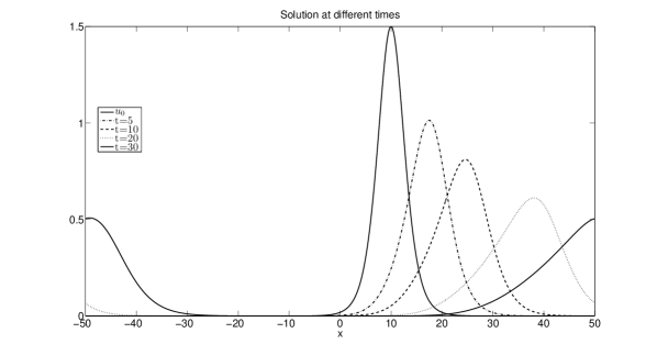
Figure 1: Solution at times $t=0$ (—), $t=5$ ($\cdot-\cdot$), $t=10$ (- - -), $t=20$ ($\cdots$), $t=30$ (—) for $\gamma_{k}=k^{2}$. Here the initial datum is the soliton.

We consider the soliton as initial datum

$$u_{0}(x)=-3(1-c)\cosh^{-2}\left(\pm\frac{1}{2}\sqrt{\frac{c-1}{c}}(x-d)\right),$$

with $c=1.5$ and $d=0.2L$ . We begin with a laplacian damping in Figure 1. The figure shows the effect of the damping on the solution. Since $\gamma_{0}=0$, the solution tends to the mean value of $u_{0}$.

Figure 2 corresponds to the simulation of the following standard dampings

• the constant: $\gamma_{k}=1,\ \forall k$,

• the laplacian: $\gamma_{k}=k^{2},\ \forall k$,

• the bilaplacian: $\gamma_{k}=k^{4},\ \forall k$.

• 

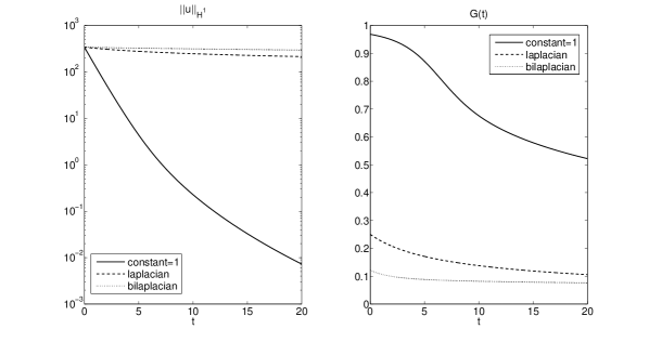
Figure 2: Evolution of $\|u\|_{H^{1}}$ and $G(t)$ with respect to time for standard dampings, the constant (—), the laplacian (- - -) and the bilaplacian ($\cdots$). Here the initial datum is the soliton.

For these dampings, we verify that the $H^{1}$-norm decreases as expected. Moreover the solution converge to the norm value of $u_{0}$ for the laplacian and bilpalacian dampings. We can also classify these dampings. Here the constant one is more efficient than the two other. But the laplacian one is more efficient than the bilaplacian one. These results are in agreement with the ones about the KdV equation [5, 8, 9, 10, 11, 14].

We extend, in Figure 3, the simulations to the dampings such that $\gamma_{k}>0$ with $\lim\limits_{k\rightarrow+\infty}\gamma_{k}=0$. We consider here three "tend to 0" dampings, with polynomial or exponential decay as follows

• $\gamma_{k}=\frac{1}{1+|k|}$,

• $\gamma_{k}=\frac{1}{(1+|k|)^{\alpha}}$, $\alpha=3$

• $\gamma_{k}=e^{-|k|}$.

These dampings do not fit with the asymptions of the theorem 2.6 but they still damp down the soliton. Indeed we notice that the $H^{1}$-norm is decreasing. We can classify the dampings. Precisely, the first one damps more than the two other and the third one is more efficient than the second one. Since these dampings tends to 0, their effects are principally on low frequencies. And for low frequencies, we have

$$\frac{1}{1+|k|}>e^{-|k|}>\frac{1}{(1+|k|)^{\alpha}}.$$

Then the classification of dampings in Figure 3 seems licit.

• 

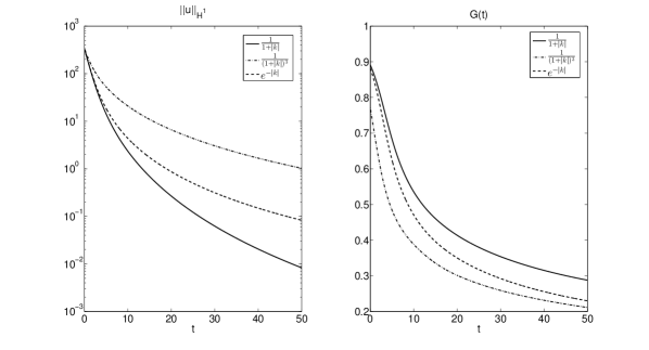
Figure 3: Evolution of $\|u\|_{H^{1}}$ and $G(t)$ with respect to time for "tend to 0" dampings, $\gamma_{k}=\frac{1}{1+|k|}$ (—), $\gamma_{k}=\frac{1}{(1+|k|)^{3}}$ ($\cdot-\cdot$) and $\gamma_{k}=e^{-|k|}$ (- - -). Here the initial datum is the soliton.

We now consider band limited dampings, namely

$$\gamma_{k}=\left\{\begin{array}[]{l}1\mbox{\leavevmode\nobreak\ if\leavevmode\nobreak\ }|k|\leq N\\ 0\mbox{\leavevmode\nobreak\ if\leavevmode\nobreak\ }|k|>N\end{array}\right.. I(N)$$ ()

We define $M:=\max(\textbf{k})$, where k is the finite vector of frequencies used for the numerical tests in Figure 4. To keep $\gamma_{k}>0,\ \forall k$, we choose

$$\gamma_{k}=\left\{\begin{array}[]{l}1\mbox{\leavevmode\nobreak\ if\leavevmode\nobreak\ }|k|\leq N\\ e^{-a||k|-N|}\mbox{\leavevmode\nobreak\ if\leavevmode\nobreak\ }|k|>N\end{array}\right.. EI(N)$$ ()

or

$$\gamma_{k}=\left\{\begin{array}[]{l}1\mbox{\leavevmode\nobreak\ if\leavevmode\nobreak\ }|k|\leq N\\ \frac{1}{\left(1+||k|-N|\right)^{a}}\mbox{\leavevmode\nobreak\ if\leavevmode\nobreak\ }|k|>N\end{array}\right.. PI(N)$$ ()

We denote the classic band limited damping by $I(N)$, the one corrected with exponential decay $EI(N)$ and the third one corrected with polynomial decay $PI(N)$. Here we set $a=3$, we obtain $\gamma_{k}>0$ with $\lim\limits_{k\rightarrow+\infty}\gamma_{k}=0$.

• 

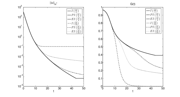
Figure 4: Evolution of $\|u\|_{H^{1}}$ and $G(t)$ with respect to time for band limited type dampings, $I\left(\frac{M}{4}\right)$ (—), $PI\left(\frac{M}{4}\right)$ (—), $EI\left(\frac{M}{4}\right)$ (—), $I\left(\frac{M}{16}\right)$ ($\cdot-\cdot$), $PI\left(\frac{M}{16}\right)$ (- - -) ,$EI\left(\frac{M}{16}\right)$ ($\cdots$). Here the initial datum is the soliton.

The difference between these dampings is when $|k|>N$. For these frequencies, since $\gamma_{k}\neq 0$, the dampings with exponential or polynomial decay should damp more than the ideal one ($I(N)$). It is the case when $N=\frac{M}{16}$, moreover the damping with polynomial decay is more effective than the one with exponential decay. But we observe similar damping when $N=\frac{N}{4}$. We notice the damping depends on the band width. It seems rightful because the equation considered is dispersive. Indeed, for this kind of equation, high frequencies appear and these frequencies cannot be damped especially if the band width is too small.

Let us illustate this by considering now the gaussian as initial datum

$$u_{0}(x)=e^{-\frac{x^{2}}{\sigma^{2}}}.$$

Here the standard deviation is fixed equal to $\sigma=\frac{\max(\textbf{k})}{10}$. Then, in order to see the effect of the damping on the low frequencies, we study the influence of the band limited damping size in Figure 5. We observe that the more $N$ increases, the more efficient is the damping. However, it seems that all dampings with $N\geq\frac{3\sigma}{2}$ behave similarly. Besides, for lower $N$, the different kind of dampings can be classified. We notice that for all $N$ and all dampings, the decreasing speed is similar at beginning and the difference appears after. The difference appears when the high frequencies does.

• 

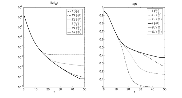
Figure 5: Evolution of $\|u\|_{H^{1}}$ and $G(t)$ with respect to time for band limited type dampings, $I\left(\frac{3\sigma}{4}\right)$ ($\cdot-\cdot$), $PI\left(\frac{3\sigma}{4}\right)$ (- - -), $EI\left(\frac{3\sigma}{4}\right)$ ($\cdots$), $I\left(\frac{3\sigma}{2}\right)$ (—), $PI\left(\frac{3\sigma}{2}\right)$ (—) ,$EI\left(\frac{3\sigma}{2}\right)$ (—). Here the initial datum is the gaussian.

The influence of the domain is finally inspected. It is known that the eigenvalues of the laplacian and of the bilapalcian depends on the length of the domain $L$. Here we choose the initial datum as

$$u_{0}(x)=\sin\left(\frac{2\pi x}{L}\right).$$

Figure 6 presents results with $L$ equal to $\pi$, $2\pi$ and $3\pi$. We notice that if $L<2\pi$, the laplacian damping is less effective than the bilaplacian one. It is the contrary if $L>2\pi$. But, the dampings are similar when $L=2\pi$. We also observe that for a fixed damping, the greater is $L$, the slower is the damping.

• 

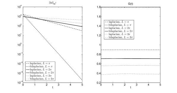
Figure 6: Evolution of $\|u\|_{H^{1}}$ and $G(t)$ with respect to time for $L=\pi$ with $\gamma_{k}=k^{2}$ ($\bm{\cdot-\cdot}$) and $\gamma_{k}=k^{4}$ (- - -), $L=2\pi$ with $\gamma_{k}=k^{2}$ (—) and $\gamma_{k}=k^{4}$ (—), $L=3\pi$ with $\gamma_{k}=k^{2}$ ($\cdots$) and $\gamma_{k}=k^{4}$ ($\cdot-\cdot$). Here the initial datum is a sine.

5 Final comments

The damping operator $\mathscr{L}_{\gamma}$ considered in this article allows to have a large variety of dampings. We first get back the standard dampings (for example $-\Delta u$). But we also have less common dampings like band-limited ones or weaker ones, e.g., such that $\lim\limits_{|k|\rightarrow+\infty}\gamma_{k}=0$. Moreover, with this frequential approach, we can adjust the dampings by frequency bands. This is interesting in order to build cheap and efficient dampings. Using these dampings, the numerical observation shows a damping for energy norms like the $H^{1}$-norm. This is consistent with the results about the asymptotic behavior.

This way of damping with frequency filters is particulary of interest for its flexibility and its efficiency. It would be a good perspective to perform similar work for the control wave equations.

References

- [1] M. Abounouh, H. Al Moatassime, J. P. Chehab, S. Dumont and O. Goubet, Discrete Schrödinger equations and dissipative dynamical systems, Commun. Pure Appl. Anal. 7 (2008), no. 2, 211–227.
- [2] C. J. Amick, J. L. Bona and M. E. Schonbek, Decay of solutions of some nonlinear wave equations, J. Differential Equations 81 (1989), no. 1, 1–49.
- [3] T. B. Benjamin, J. L. Bona and J. J. Mahony, Model equations for long waves in nonlinear dispersive systems, Philos. Trans. Roy. Soc. London Ser. A 272 (1972), no. 1220, 47–78.
- [4] M. Cabral and R. Rosa, Chaos for a damped and forced KdV equation, Phys. D 192 (2004), no. 3-4, 265–278.
- [5] J.-P. Chehab and G. Sadaka, Numerical study of a family of dissipative KdV equations, Commun. Pure Appl. Anal. 12 (2013), no. 1, 519–546.
- [6] J.-P. Chehab and G. Sadaka, On damping rates of dissipative KdV equations, Discrete Contin. Dyn. Syst. Ser. S 6 (2013), no. 6, 1487–1506.
- [7] A. Durán and J. M. Sanz-Serna, The numerical integration of relative equilibrium solutions. The nonlinear Schrödinger equation, IMA J. Numer. Anal. 20 (2000), no. 2, 235–261.
- [8] J.-M. Ghidaglia, Weakly damped forced Korteweg-de Vries equations behave as a finite-dimensional dynamical system in the long time, J. Differential Equations 74 (1988), no. 2, 369–390.
- [9] J.-M. Ghidaglia, A note on the strong convergence towards attractors of damped forced KdV equations, J. Differential Equations 110 (1994), no. 2, 356–359.
- [10] O. Goubet, Asymptotic smoothing effect for weakly damped forced Korteweg-de Vries equations, Discrete Contin. Dynam. Systems 6 (2000), no. 3, 625–644.
- [11] O. Goubet and R. M. S. Rosa, Asymptotic smoothing and the global attractor of a weakly damped KdV equation on the real line, J. Differential Equations 185 (2002), no. 1, 25–53.
- [12] N. Hayashi, E. I. Kaikina and P. I. Naumkin, Large time asymptotics for the BBM-Burgers equation, Ann. Henri Poincaré 8 (2007), no. 3, 485–511.
- [13] D. J. Korteweg and G. de Vries, On the change of form of long waves advancing in a rectangular canal and on a new type of long stationnary waves, Phil. Maj. 39 (1895), 422-443.
- [14] E. Ott and R.N. Sudan, Damping of solitary waves, The Physics of fluids 13 (1970), no. 6.
- [15] R. Temam, Infinite-dimensional dynamical systems in mechanics and physics, second edition, Applied Mathematical Sciences, 68, Springer, New York (1997).
- [16] S. Vento, Global well-posedness for dissipative Korteweg-de Vries equations, Funkcial. Ekvac. 54 (2011), no. 1, 119–138.
- [17] S. Vento, Asymptotic behavior of solutions to dissipative Korteweg-de Vries equations, Asymptot. Anal. 68 (2010), no. 3, 155–186.
- [18] B. Wang, Strong attractors for the Benjamin-Bona-Mahony equation, Appl. Math. Lett. 10 (1997), no. 2, 23–28.