High-resolution calculations of the solar global convection with the reduced speed of sound technique: I. The structure of the convection and the magnetic field without the rotation.

Abstract

We carry out non-rotating high-resolution calculations of the solar global convection, which resolve convective scales of less than 10 Mm. To cope with the low Mach number conditions in the lower convection zone, we use the reduced speed of sound technique (RSST), which is simple to implement and requires only local communication in the parallel computation. In addition, the RSST allows us to expand the computational domain upward to about $0.99R_{\odot}$ as it can also handle compressible flows. Using this approach, we study the solar convection zone on the global scale, including small-scale near-surface convection. In particular, we investigate the influence of the top boundary condition on the convective structure throughout the convection zone as well as on small-scale dynamo action. Our main conclusions are: 1. The small-scale downflows generated in the near-surface layer penetrate into deeper layers to some extent and excite small-scale turbulence in the region $>0.9R_{\odot}$, where $R_{\odot}$ is the solar radius. 2. In the deeper convection zone ($<0.9R_{\odot}$), the convection is not influenced by the location of the upper boundary. 3. Using an LES approach, we can achieve small-scale dynamo action and maintain a field of about $0.15-0.25B_{\mathrm{eq}}$ throughout the convection zone, where $B_{\mathrm{eq}}$ is the equipartition magnetic field to the kinetic energy. 4. The overall dynamo efficiency varies significantly in the convection zone as a consequence of the downward directed Poynting flux and the depth variation of the intrinsic convective scales.

1 INTRODUCTION

The solar convection zone is filled with turbulent thermal convection due to its superadiabatic stratification, which is maintained by the radiative energy flux from the core of the Sun. Due to the influence of rotation, the anisotropic convection transports angular momentum as well as energy. This maintains mean flows such as the meridional flow and the differential rotation. These flows are thought to be important for the dynamo and related eleven-year cyclic variations of the sunspot numbers (Parker 1955; Choudhuri et al. 1995; Dikpati & Charbonneau 1999; Hotta & Yokoyama 2010a, b). In addition, the turbulent thermal convection itself is also important for the generation of the magnetic field. Idealized simulations (e.g., Brandenburg et al. 1996; Cattaneo 1999) and the realistic calculations for the photosphere (Vögler & Schüssler 2007; Pietarila Graham et al. 2010) have suggested that chaotic motions have the ability to maintain magnetic energy through a small-scale dynamo process. Such dynamos have not been studied so far on the the global scale, i.e., the entire convection zone.

The purpose of this study is to achieve multi-scale convection, including scales from $10$ Mm (smaller than supergranulation) up to $\sim 200$ Mm (global scale). We accomplish this by approaching the solar surface up to $0.99R_{\odot}$ using unprecedented resolution, studying in particular the influence of the location of the upper boundary on the convective structure in the deeper parts of the convection zone. In addition, we use our approach to study the transport and the generation of the magnetic field by turbulent convection in the absence of rotation, i.e., we study the operation of a small-scale dynamo in the highly stratified convection zone.

The paper is organized as follows: We provide an overview of the reduced speed of sound technique in §2, introduce our numerical setting in §3, and show the results in §4,present the properties based on the obtained spatial distributions in §4.1, discuss the energy balance using the integrated flux in §4.2, analyze , the properties of the convection in cases without the magnetic fields using the spherical harmonic expansion in §4.3, and analyze the cases with magnetic fields using spherical harmonic expansion and the probability density function in §4.4, investigate the transportation and the generation of the magnetic field in the convection zone in §4.5, and summarize our investigation in §5.

2 Reduced speed of sound technique

Developing numerical simulations of solar global convection is challenging due to the high resolution and the broad range of dynamical time scales that are required. One of the most paramount difficulties arises from the high speed of sound and the related low Mach-number flows throughout most of the convection zone. At the base of the convection zone, the speed of sound is about $200\ \mathrm{km\ s^{-1}}$, while the speed of convection is thought to be $50\ \mathrm{m\ s^{-1}}$ (e.g., Stix 2004). The time step must therefore be shorter owing to the CFL (Courant-Friedrichs-Lewy) condition in an explicit fully compressible method, even when we are interested in the phenomena related to convection. In order to avoid this situation, the anelastic approximation is frequently adopted in which the mass conservation equation is replaced with $\nabla\cdot(\rho_{0}{\bf v})=0$, where $\rho_{0}$ is the reference density and ${\bf v}$ is the fluid velocity. In this approximation, the speed of sound is assumed to be infinite, and we need to solve the elliptic equation for the pressure, which filters out the propagation of the sound wave. Since the anelastic approximation is well applicable deep in the convection zone and the time step is no longer limited by the large speed of sound, the solar global convection has been investigated with this method in numerous studies about the differential rotation, the meridional flow, the global dynamo, and the dynamical coupling of the radiative zone (Miesch et al. 2000, 2006, 2008; Brun & Toomre 2002; Brun et al. 2004, 2011; Browning et al. 2006; Ghizaru et al. 2010).

There are, however, two drawbacks in the anelastic approximation. The first is the breakdown of the approximation near the solar surface. Since the convection velocity becomes higher and the speed of sound becomes lower in the near-surface layer ($>0.98R_{\odot}$), these have similar values and the anelastic approximation cannot be applied. Since the interaction between the small-scale convection generated in the near-surface layer (granulation and supergranulation) and large scale convection (giant cell and global one) is an important topic, the connection between the near-surface layer and the global convection has been investigated (e.g., Augustson et al. 2011). The global calculation, however, which includes all such multiple scales, has not been achieved yet. The second drawback is the difficulty arising from the increase of the required resolution. The pseudo-spectral method based on the spherical harmonic expansion is frequently adopted, especially for solving the elliptic equation of the pressure. In this method, non-linear terms require the transformation of the physical variable from the real space to the spectral space, and vice versa every time step. The calculation cost of the transformation is estimated as $\mathcal{O}(N_{\theta}^{2}N_{\phi}\log N_{\phi})$ due to the absence of a fast algorithm for the Legendre transformation, which is as powerful as the fast Fourier transformation (FFT), where $N_{\theta}$ and $N_{\phi}$ are the maximum mode numbers in the latitude and the longitude respectively. Thus the computational cost of this method is significant, limiting the achievable resolution. Owing to this, some numerical calculations of the geodynamo adopt the finite difference method in order to achieve high resolution (Kageyama et al. 2008; Miyagoshi et al. 2010). As explained above, when the near-surface layer is included in the calculation, the typical convection scale becomes small and a large number of grid points is required. The resolution is one of the keys to access the solar surface. We note that some studies using the finite difference have been done in the stellar or solar context using a moderate ratio of the speed of sound and the convection velocity with adjustments of the radiative flux and the stratification (Käpylä et al. 2011, 2012). Although this type of approach provides insights for the maintenance of the mean flow and the magnetic field, proper reproduction using the solar parameters, such as the stratification, the luminosity, the partial ionization effect and the rotation, and direct comparison with actual observations cannot be achieved.

The reduced speed of sound technique (hereafter RSST, Rempel 2005, 2006; Hotta et al. 2012b) can overcome these drawbacks while avoiding the severe time step caused by the speed of sound. In the RSST the equation of continuity is replaced with

$$\frac{\partial\rho}{\partial t}=-\frac{1}{\xi^{2}}\nabla\cdot(\rho{\bf v}).$$ (1)

The speed of sound is then reduced $\xi$ times, but the dispersion relationship for sound waves remains (where wave speed decreases equally for all wavelengths). This technique does not change the hyperbolic character of the equations that can be integrated explicitly. Due to this hyperbolicity, only the local communication is required, which decreases the communication overhead in parallel computing. A simple algorithm and low cost of communication are significant factors that enable high resolution calculations. Hotta et al. (2012b) investigated the validity of the RSST in a thermal convection problem. It was concluded that the RSST is valid when the Mach number defined with the RMS (root mean square) velocity and the reduced speed of sound $\hat{c_{s}}$ is smaller than 0.7. Another advantage of this method is its accessibility to the real solar surface with an inhomogeneous $\xi$. The Mach number varies substantially in the solar convection zone. When a moderate or zero reduction of the speed of sound is used in the near-surface layer while a large $\xi$ around the bottom part of the convection zone is used, the properties of the thermal convection, even including the surface, can be properly investigated without undermining the physics. Hotta et al. (2012b) confirmed that the inhomogeneous $\xi$ is valid again when the Mach number is less than 0.7.

3 MODEL

We solve the three-dimensional magnetohydrodynamic equations with the RSST in the spherical geometry $(r,\theta,\phi)$ as:

$$\frac{\partial\rho_{1}}{\partial t}=-\frac{1}{\xi^{2}}\nabla\cdot\left(\rho_{0}{\bf v}\right),$$ (2)

$$\rho_{0}\frac{\partial{\bf v}}{\partial t}=-\rho_{0}({\bf v}\cdot\nabla){\bf v}-\nabla\left(p_{1}+\frac{B^{2}}{8\pi}\right)+\nabla\cdot\left(\frac{{\bf BB}}{4\pi}\right)-\rho_{1}g{\bf e_{r}},$$ (3)

$$\frac{\partial{\bf B}}{\partial t}=\nabla\times\left({\bf v}\times{\bf B}\right),$$ (4)

$$\rho_{0}T_{0}\frac{\partial s_{1}}{\partial t}=-\rho_{0}T_{0}({\bf v}\cdot\nabla)s_{1}+\frac{1}{r^{2}}\frac{d}{dr}\left(r^{2}\kappa_{\mathrm{r}}\rho_{0}c_{\mathrm{p}}\frac{dT_{0}}{dr}\right)+\Gamma,$$ (5)

where $\rho$, $p$, $s$, $T$, ${\bf v}$, and ${\bf B}$ are the density, the gas pressure, the specific entropy, the temperature, the fluid velocity and the magnetic field, respectively. The subscript 1 denotes the fluctuation from the time-independent spherically symmetric reference state, which has subscript 0. $g$, $\kappa_{\mathrm{r}}$, and $\Gamma$ are the gravitational acceleration, the coefficient of the radiative diffusivity, and the surface cooling term, respectively. The setting of these values is explained in the following paragraph. In order to close the MHD system, we adopt a non-ideal equation of state as:

$$p_{1}=\left(\frac{\partial p}{\partial\rho}\right)_{s}\rho_{1}+\left(\frac{\partial p}{\partial s}\right)_{\rho}s_{1}.$$ (6)

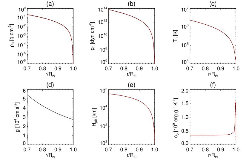
Figure 1: The values at the reference state, (a) the density, (b) the gas pressure, (c) the temperature, (d) the gravitational acceleration, (e) the pressure scale height, (f) the heat capacity at constant pressure, are shown. The black and red lines show the reference state in our study and the values from Model S, respectively. The value of the gravitational acceleration in this study is exactly the same as in Model S.

Since our upper boundary is at $r=0.99R_{\odot}$ at maximum, in the near-surface region partial ionization is important (see Fig. 1f) and is included in our treatment (see Appendix A for details) by using the OPAL repository with the solar abundance of $X=0.75$, $Y=0.23$, and $Z=0.02$, where $X$, $Y$, and $Z$ specify the mass fraction of hydrogen, helium and other metals, respectively.

Note that we do not have any explicit turbulent thermal diffusivity and viscosity (Miesch et al. 2000) in order to maximize the fluid and magnetic Reynolds number, but use the artificial viscosity introduced in Rempel et al. (2009). Our treatment ensures that the dissipated kinetic and magnetic energies with the artificial viscosity are converted to the internal energy. Note also that the rotation is not included in this study, since we focus on the connection of thermal convection between the small and large scales and its local dynamo action on the global scale. The combination of rotation and stratified convection leads to differential rotation and additional turbulent induction effects that enable large-scale dynamo action. It is difficult to distinguish the local dynamo action from global dynamo action if rotation is present. Since the rotation effect in the sun is significant, we will carry out studies of rotating convection in the future.

Fig. 1 shows our reference state in comparison with Model S (Christensen-Dalsgaard et al. 1996). The reference stratification is determined by solving the one-dimensional hydrostatic equation and the realistic equation of state as:

$$\frac{dp_{0}}{dr}=-\rho_{0}g,$$ (7)

$$\rho_{0}=\rho_{0}(p_{0},s_{0}),$$ (8)

$$\frac{ds_{0}}{dr}=0.$$ (9)

Eq. (8) is calculated with the OPAL repository including partial ionization. We set an adiabatic stratification as a reference and initial state. The stratification becomes superadiabatic after convection develops as a consequence of radiative heating near the bottom and radiative cooling at the top as described below. The gravitational acceleration and the radiative diffusion are adopted from Model S. The boundary is set at $r=0.998R_{\odot}$ with the values from Model S, and the equations are integrated inward.

On the actual Sun, the surface is continuously cooled by the radiation. Since our boundary is not located on the real solar surface (even though it is unprecedentedly closer to the real surface), we add an artificial cooling ($\Gamma$) as:

$$\Gamma(r)=-\frac{1}{r^{2}}\frac{\partial}{\partial r}(r^{2}F_{\mathrm{s}}),$$ (10)

where

$$r^{2}F_{\mathrm{s}}(r)=r^{2}_{\mathrm{min}}F_{\mathrm{r}}(r_{\mathrm{min}})\exp\left[-\left(\frac{r-r_{\mathrm{max}}}{d_{\mathrm{c}}}\right)^{2}\right],$$ (11)

$$F_{\mathrm{r}}(r)=-\kappa_{\mathrm{r}}\rho_{0}c_{\mathrm{p}}\frac{dT_{0}}{dr},$$ (12)

where $r_{\mathrm{min}}$ and $r_{\mathrm{max}}$ denote the location of the bottom and the top boundary, respectively. This procedure ensures that the radiative luminosity imposed at the bottom is released through the top boundary. Since the realistic simulation for the near-surface layer shows that the thickness of the cooling layer by the radiation is similar to the local pressure scale height (e.g. Stein et al. 2009), we adopt two pressure scale heights for the thickness of the cooling layer, i.e., $d_{\mathrm{c}}=2H_{p0}(r_{\mathrm{max}})$ except for cases H1 and M1 (see table 1), where $H_{p0}=p_{0}/(\rho_{0}g)$ is the pressure scale height.

We carry out three calculations named H0, H1 and H2, with different settings that are primarily hydrodynamic. In case H0, the top boundary is located at $r=0.99R_{\odot}$, and the density contrast $\rho_{0}(r_{\mathrm{min}})/\rho_{0}(r_{\mathrm{max}})$ exceeds 600. To our knowledge, this is the largest value achieved so far in numerical simulations of solar global convection. In cases H1 and H2, the top boundary is at $r=0.96R_{\odot}$, and the density contrast is around 40. In case H1, the thickness of the cooling layer is the same as case H0, i.e., $d_{\mathrm{c}}=3740\ \mathrm{km}$, which is the two pressure scale heights at $r=0.99R_{\odot}$, while case H2 adopts two scale heights at its top boundary ($r_{\mathrm{max}}=0.96R_{\odot}$) for the thickness ($d_{\mathrm{c}}$). Our magnetic runs M0, M1 and M2 use the same settings and differ only through the initial magnetic field added. We note that the thickness of the cooling layer ($d_{\mathrm{c}}$) has almost the same role as the value of the turbulent thermal diffusivity on the entropy that is adopted in the ASH simulation (Miesch et al. 2000, 2008).

In this study, the factor of the RSST is set to make the adiabatic reduced speed of sound uniform in space. The adiabatic speed of sound is defined as:

$$c_{\mathrm{s}}(r)=\sqrt{\left(\frac{\partial p}{\partial\rho}\right)_{s}}.$$ (13)

Then the factor of the RSST is set as:

$$\xi(r)=\xi_{0}\frac{c_{\mathrm{s}}(r)}{c_{\mathrm{s}}(r_{\mathrm{min}})}.$$ (14)

In this study, we adopt $\xi_{0}=120$ for all the calculations, thus the reduced speed of sound ${\hat{c}_{\mathrm{s}}}\equiv c_{\mathrm{s}}/\xi=1.88\ \mathrm{km\ s^{-1}}$ at all depths. Hotta et al. (2012b) suggest that the RSST is valid for the thermal convection under the criterion of $v_{\mathrm{rms}}/\hat{c}_{\mathrm{s}}<0.7$, where $v_{\mathrm{rms}}$ is the RMS (root mean square) convection velocity. Thus we can properly treat the convection with $v_{\mathrm{rms}}<1.3\ \mathrm{km\ s^{-1}}$ in this model. It is also suggested in Hotta et al. (2012b) that the total mass is not conserved with the inhomogeneous $\xi$, and we cannot avoid long-term drift from the reference state, i.e., the mass continuously decreases or increases. In this study, however, we adopt a different way to avoid this type of long-term drift. When the equation of continuity is treated as:

$$\frac{\partial}{\partial t}\left(\xi^{2}\rho_{1}\right)=-\nabla\cdot\left(\rho_{0}{\bf v}\right),$$ (15)

the value $\hat{M}$ is conserved in a rounding error with appropriate boundary conditions, where

$$\hat{M}=\int_{V}\xi^{2}\rho_{1}dV.$$ (16)

Although the radial distribution of the density is different from the original one, the fluctuation part remains small (e.g. $\rho_{1}/\rho_{0}\sim 10^{-6}$), and this does not affect the character of the thermal convection. It is confirmed in Hotta et al. (2012b) that statistical features are not influenced by the inhomogeneous $\xi$.

We use the stress-free and the impenetrable boundary conditions for the fluid velocity, $v_{r}$, $v_{\theta}$, and $v_{\phi}$. The free boundary condition is adopted for the density and the entropy, i.e., $\partial\rho_{1}/\partial r=\partial s_{1}/\partial r=0$. The magnetic field is vertical at the top boundary, and the perfect conductor boundary condition is used at the bottom boundary.

$\rho_{1}$, $B_{r}$, $B_{\theta}$, $B_{\phi}$ and $s_{1}$ are zero initially. The fluid velocities $v_{r}$, $v_{\theta}$, and $v_{\phi}$ have small random values. After the convection reaches a statistically steady state, a uniform magnetic field ($B_{\phi}=100\ \mathrm{G}$) is added. Although a net toroidal flux exists initially using this condition, it disappears through the upper boundary after around $75$ days, since horizontal magnetic field is zero there. Thus we do not need to consider the influence of the net flux for our local dynamo study.

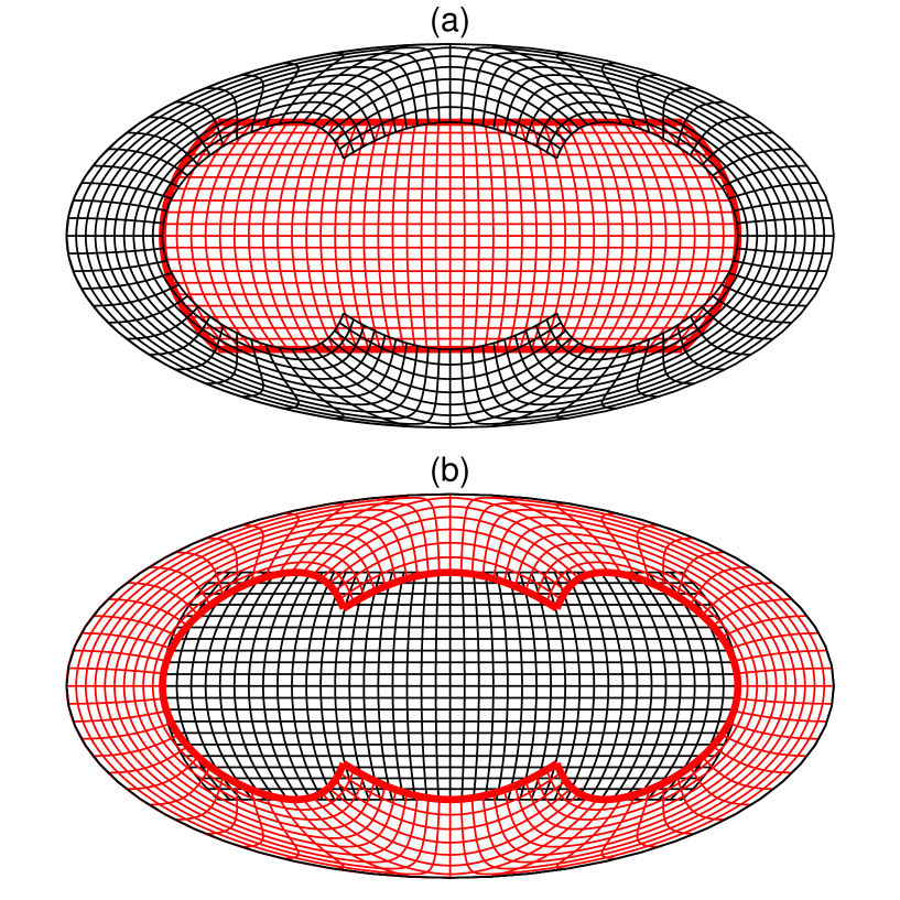
Figure 2: Red lines and black lines indicate the Yin and Yang grid, respectively. (a) and (b) show the geometry on the mollweide projection from the different viewpoints. The thick red lines show the boundaries for both the Yin and Yang grids.

Under the setting explained above, we solve the equations (2)-(5) by using the fourth-order Runge-Kutta scheme for the time-integration and the fourth-order space-centered derivative (Vögler et al. 2005). The divergence free condition, i.e., $\nabla\cdot{\bf B}=0$, is maintained with the diffusion scheme for each Runge-Kutta loop (see the Rempel et al. (2009) appendix for details). In order to include all the spherical shell, we adopt the Yin-Yang grid (Kageyama & Sato 2004). The Yin-Yang grid is a set of two congruent spherical geometries. They are combined in a complemental way to cover a whole spherical shell. The boundary condition for each grid is calculated using the interpolation of the other grid. In all of our calculations, each grid covers $0.715R_{\odot}<r<r_{\mathrm{max}}$, $\pi/4-\delta_{\theta}<\theta<3\pi/4+\delta_{\theta}$, and $-3\pi/4-\delta_{\phi}<\phi<3\pi/4+\delta_{\phi}$, where $\delta_{\theta}$ and $\delta_{\phi}$ are the margins for the interpolation. Here $\delta_{\theta}=3\Delta\theta/2$ and $\delta_{\phi}=3\Delta\phi/2$ are adopted for the interpolation with the third-order function, where $\Delta\theta$ and $\Delta\phi$ are the grid spacing in the latitudinal and longitudinal directions. Here $r=0.715R_{\odot}=r_{\mathrm{min}}$ is the location of the base of the convection zone and $r_{\mathrm{max}}$ is taken as a parameter ($r_{\mathrm{max}}=0.99R_{\odot}$ for the typical case). Although the boundary condition for the Yin grid is applied on the edge of the Yin grid, the boundary condition for the Yang grid is applied on the edge of the Yin grid in order to avoid the double solution in the overlapping area of the Yin-Yang grid. Fig. 2 shows this configuration. The thick red lines show the location of the horizontal boundary for both Yin and Yang grids.

The horizontal grid spacing is 1,100 km at the top boundary and 375 km radially. With the Yin-Yang geometry, the number of grid points is $1024(N_{\theta})\times 3072(N_{\phi})\times 2$. The last factor 2 indicates a Yin and Yang pair. The number of grid points in the radial direction is shown in Table 1. Since this resolution in Yin-Yang geometry has almost the same quality as that of $512(r)\times 2048(\theta)\times 4096(\phi)$ in ordinary spherical geometry in cases H0 and M0, we succeed in doubling the resolution in each direction from the previous study (Miesch et al. 2008). After the uniform magnetic field is added, the calculations are newly named M0, M1 and M2, which use the results of H0, H1, and H2, respectively. Using a hybrid MPI and automatic intra-node parallelization approach, the code scales efficiently up to $10^{5}$ cores with almost linear weak scaling, and achieves a 14% performance at maximum on the RIKEN K-computer in Japan. Since our code includes almost no global communication among cores, this linear scaling is expected to hold further with larger core counts.

4 Results

4.1 Structure of convection and the magnetic field

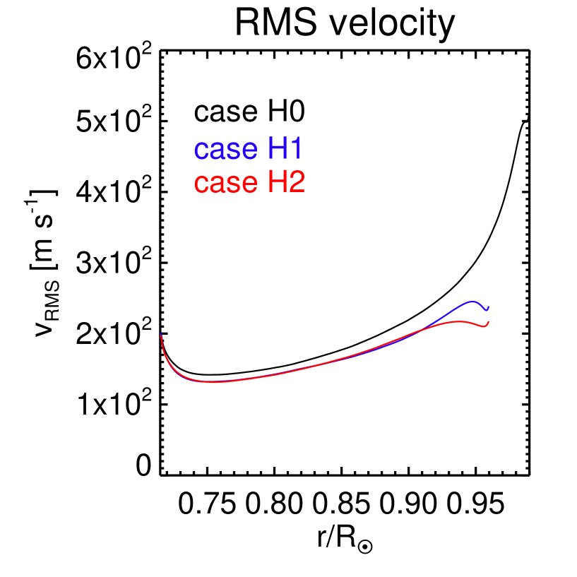
Figure 3: RMS (root mean square) velocities as a function of the depth are shown. The black, blue, and red lines show the results in cases H0, H1, and H2, respectively.

Fig. 3 shows the RMS velocities in cases H0, H1, and H2. The maximum RMS velocity is $5\times 10^{2}\ \mathrm{m\ s^{-1}}$ at the top boundary in case H0. Since the Mach number determined with the reduced speed of sound $\hat{c}_{\mathrm{s}}$ is always under 0.3 throughout the convection zone, the requirement for the validity of the RSST in this study is well satisfied (Hotta et al. 2012b). The difference between cases H1 and H2 is mostly a local effect. The thinner cooling layer in case H1 leads to stronger acceleration of plasma and causes a higher RMS velocity close to the top boundary. In case H0 the RMS velocity is significantly larger in the near surface layer ($>0.96R_{\odot}$), since the energy has to be transported with a small background density. This has some influence on the velocity throughout the convection zone.

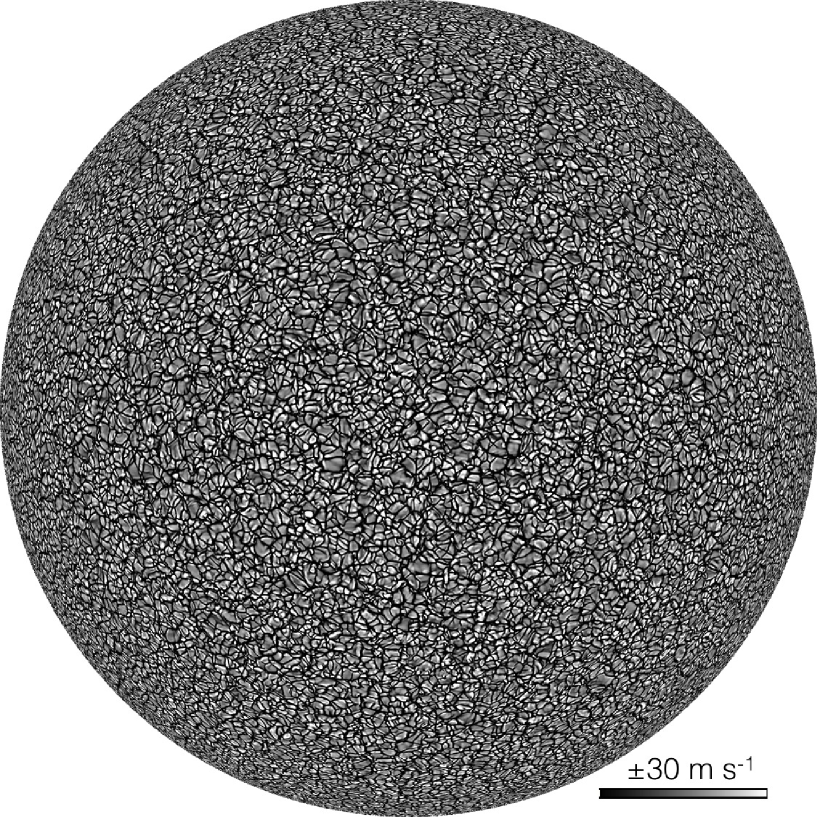
Figure 4: The radial velocity ($v_{r}$) in case H0 on the orthographic projection. The movie is provided online.

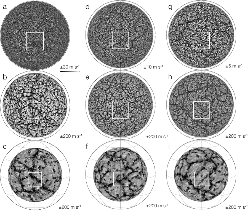
Figure 5: The radial velocities ($v_{r}$) are shown at $r=r_{\mathrm{max}}$ (a,d,g), $r=0.95R_{\odot}$ (b,e,h) and $r=0.85R_{\odot}$ (c,f,i). The results in cases H0, H1, and H2 are shown in (a,b,c), (d,e,f), and (g,h,i), respectively. The black circle around each panel shows the location at $r=R_{\odot}$.

Fig. 4 shows the radial velocity ($v_{r}$) around the top boundary in case H0 ($r_{\mathrm{max}}=0.99R_{\odot}$, which is 7 Mm below the photosphere) in the orthographic projection. (The corresponding movie is provided online.) Note that since the shown location is close to the impenetrable top boundary, the value of the radial velocity is rather small. Since in the area near the upper boundary the pressure scale height is less than 2 Mm, the convection pattern shows significantly small cells of about $\sim 7\ \mathrm{Mm}$. The typical cell size is slightly smaller than the supergranulation that is observed in the photosphere. This study is the first that well resolves the 10 Mm-scale convection pattern in a calculation of the solar global convection zone. Fig. 5a-c shows the radial velocity at $r=0.99R_{\odot}$, $r=0.95R_{\odot}$, and $r=0.85R_{\odot}$ in case H0 by using the orthographic projection. In deeper layers the pressure scale height becomes larger (see Fig. 1e) and the convection cell increases in size. A detailed analysis using the spherical harmonic expansion of the convective structure is shown in §4.3.

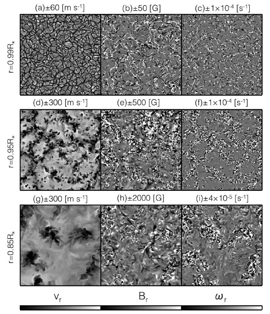
Figure 6: The zoomed-in contour of the radial velocity ($v_{r}$: left panels), the radial magnetic field ($B_{r}$: middle panels) and the radial vorticities ($\omega_{r}$: right panels) at different depths. The field of view is $30^{\circ}$ both in the latitude and the longitude, which corresponds to the size of 370 Mm at the top boundary.

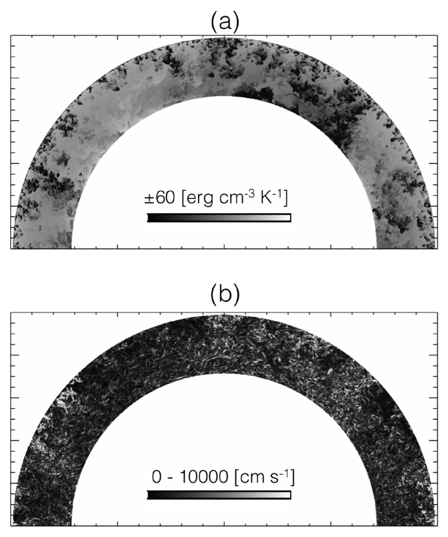
Figure 7: (a) $\rho_{0}[s_{1}-\langle s_{1}\rangle]$, and (b) $B/\sqrt{4\pi\rho_{0}}$ on the meridional plane at $\phi=0$, where $\langle{s}\rangle$ is the horizontal average of the entropy.

Figs. 6a, d, and g show the zoomed-up contour of the radial velocity in case M0, i.e., after the inclusion of the magnetic field in H0. The region is indicated by the white rectangle in Figs. 5a-c. Figs. 6c, f, and i show the vorticity ($\omega_{r}=(\nabla\times{\bf v})_{r}$) at $r=0.99R_{\odot}$, $0.95R_{\odot}$, and $0.85R_{\odot}$, respectively. As already seen in case H0 (Fig. 5), it is clear that the scale of the thermal convection pattern significantly depends on the depth. In addition, the large-scale downflow is associated with the small-scale and strong vorticity in the deeper layer (especially in $r=0.85R_{\odot}$). Fig. 7a shows $\rho_{0}[s_{1}(r,\theta,\phi=0)-\langle s_{1}\rangle]$ in the meridional plane, where $\langle s_{1}\rangle$ is the horizontal average of the entropy. The low and high entropy materials correspond to the downflow and upflow, respectively. In the near-surface region, the convection structure shows a combination of broad upflows and narrow downflows $\sim 7\ \mathrm{Mm}$ forming at the top boundary. These small-scale downflows merge in the middle of the convection zone and build large-scale downflow. Although the overall structure of such convection is large, there is a superimposed turbulent pattern especially in the downflow region, which is shown in Fig. 6.

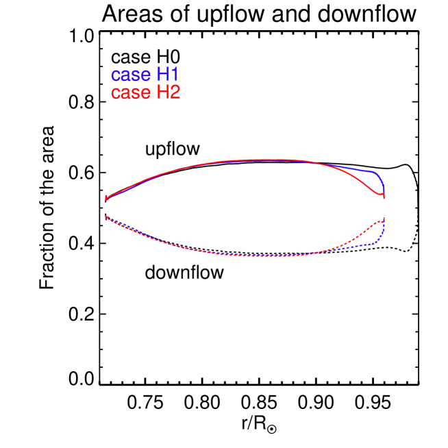
Figure 8: The occupied fraction of the area of the upflow (solid line) and downflow (dashed line). The black, blue and red lines show the results in cases H0, H1, and H2, respectively.

Figs. 5d, e, and f show the results of case H1 with a different location of the top boundary ($r_{\mathrm{max}}=0.96R_{\odot}$) at $r=r_{\mathrm{max}}$, $r=0.95R_{\odot}$, and $r=0.85R_{\odot}$, respectively. Since the location and the pressure scale height of the shown images is different between case H0 in Figs. 5a ($r=r_{\mathrm{max}}=0.99R_{\odot}$) and H1 in d ($r=r_{\mathrm{max}}=0.96R_{\odot}$), it is natural that the convective structures are much different, i.e., those in H0 have smaller scale convection than in H1. It is more important that the structures at the same depth, $0.95R_{\odot}$, are significantly different from each other between these cases (H0 in Fig. 5b and H1 in Fig. 5e. The small-scale downflow plumes penetrate near the surface layer and influence its structure (see also Fig. 7a). When the downflow goes deeper, the influence becomes smaller. This is seen in the comparison of Figs. 5c ($r_{\mathrm{max}}=0.99R_{\odot}$ and $r=0.85R_{\odot}$) and f ($r_{\mathrm{max}}=0.96R_{\odot}$ and $r=0.85R_{\odot}$), where the difference of convection structure seems insignificant. Figs. 5g, h, and i show the results in case H2, in which the location of the top boundary is the same as in H1 but the thickness of the cooling layer is larger. The convective structure around the top boundary shows the largest scale (Fig. 5g), while again the difference becomes smaller in the deeper layer (Fig. 5c, f, and i). This is also shown in Fig. 8 by the areas occupied by the upflow and the downflow, i.e., positive and negative radial velocities ($v_{r}$). Up to the middle of the convection zone ($<0.9R_{\odot}$), cases H0, H1 and H2 all show similar behavior, i.e., the fractional area by the upflow is larger ($\sim 65\%$) but decreases below $\sim 0.85R_{\odot}$ to equal to that of the downflow. Interestingly, this behavior is quantitatively the same in spite of the significant difference between H0 and H1 in the density contrast (see table 1).

4.2 Integrated energy flux

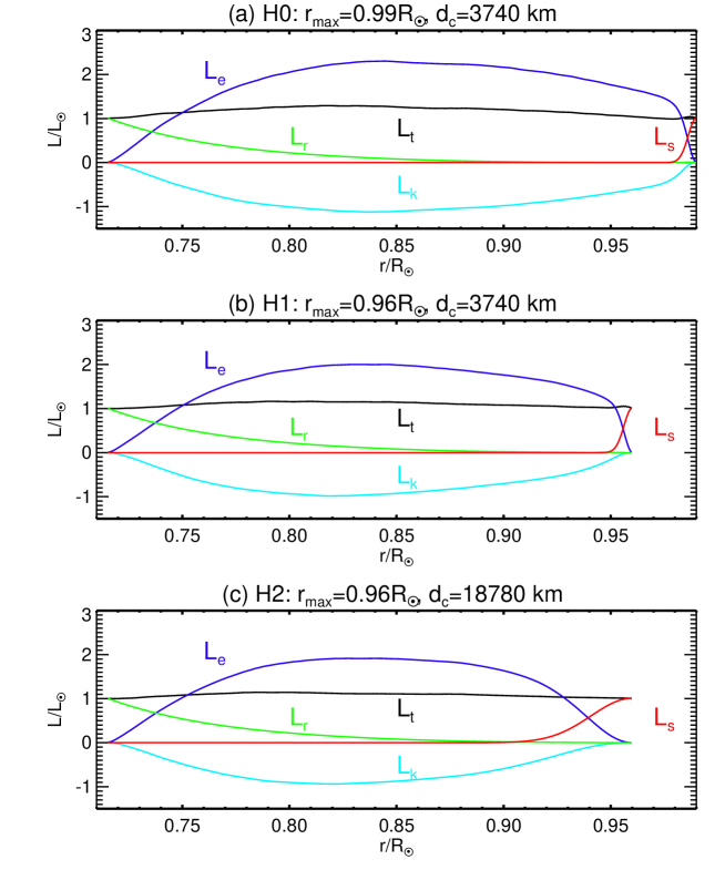
Figure 9: The integrated fluxes are shown. Panels a, b, and c show the results in cases H0, H1, and H2, respectively. The black, blue, green, red, and light blue lines show the total, enthalpy, radiative, surface cooling, and kinetic fluxes, respectively.

Fig. 9 shows the integrated fluxes. The integrated enthalpy flux ($L_{\mathrm{e}}$), the integrated kinetic flux ($L_{\mathrm{k}}$), the radiative luminosity ($L_{\mathrm{r}}$) and the luminosity form of the surface cooling ($L_{\mathrm{s}}$) are defined as:

$$L_{\mathrm{e}} = \int_{s}\left[\rho_{0}e_{1}+p_{1}-\frac{p_{0}\rho_{1}}{\rho_{0}}\right]v_{r}dS,$$ (17)

$$L_{\mathrm{k}} = \int_{s}\frac{1}{2}\rho_{0}v^{2}v_{r}dS,$$ (18)

$$L_{\mathrm{r}} = \int_{s}F_{\mathrm{r}}(r)dS,$$ (19)

$$L_{\mathrm{s}} = \int_{s}F_{\mathrm{s}}(r)dS.$$ (20)

The radiative flux ($F_{\mathrm{r}}$) and surface cooling flux ($F_{\mathrm{s}}$) are defined in eq. (11) and eq. (12), respectively. The derivation of the enthalpy flux is given in Appendix B. Fig. 9a shows the integrated fluxes in case H0 ($r_{\mathrm{max}}=0.99R_{\odot}$ and $d_{\mathrm{c}}=3740\ \mathrm{km}$). The total integrated flux $L_{\mathrm{t}}=L_{\mathrm{e}}+L_{\mathrm{k}}+L_{\mathrm{r}}+L_{\mathrm{s}}$ is almost constant along the depth. This indicates that the convection zone in our calculation is in energy equilibrium. This takes about 50 days. Note that since we do not use a conservative form for the total energy nor estimate the energy flux contributions caused by the artificial diffusivities, the total flux is not completely constant. The enthalpy flux transports twice the solar luminosity upward at maximum, and the kinetic flux transports almost the same amount of the energy as the solar luminosity downward at maximum. Although the kinetic energy flux is frequently ignored in the one-dimensional mixing length model (e.g. Stix 2004), our result shows the importance of the kinetic flux. This has been already suggested by Miesch et al. (2008). Figs. 9b, and c show the results in cases H1 and H2, respectively. The integrated fluxes show almost the similar behavior as those in case H0, but the maximum absolute values of the enthalpy and kinetic flux are smaller. Since these absolute values gradually decrease from H0 to H2, we conclude that both the thickness of the cooling layer and the location of the upper boundary contribute to this result. It is possible that when the upper boundary becomes closer to the real solar surface and the cooling layer becomes thinner, the absolute values of the enthalpy flux and the kinetic flux become even larger than our case H0.

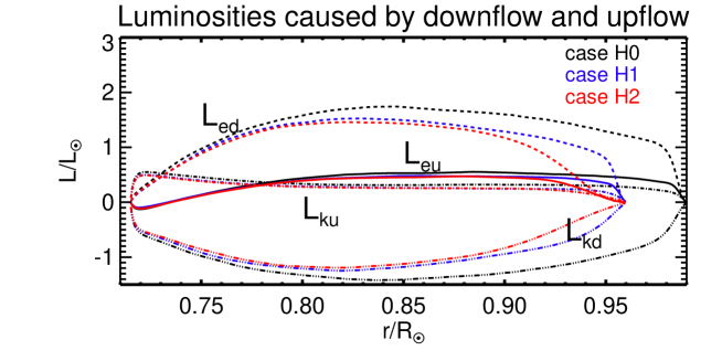
Figure 10: The enthalpy and kinetic flux transported by the upflow ($L_{\mathrm{eu}}$ and $L_{\mathrm{ku}}$) and the downflow ($L_{\mathrm{ed}}$ and $L_{\mathrm{eu}}$) are shown. The black, blue and red lines show the results in cases H0, H1, and H2, respectively. The solid and dashed lines indicate the enthalpy flux in the upflow and the downflow, respectively, and the dash-dot and dash-dot-dot-dot lines indicate the kinetic energy flux in the upflow and the downflow, respectively.

Fig. 10 shows the integrated enthalpy flux and the kinetic flux transported by upflow ($L_{\mathrm{eu}}$, $L_{\mathrm{ku}}$) and downflow ($L_{\mathrm{ed}}$, $L_{\mathrm{kd}}$), respectively. Note that the enthalpy flux by upflow and downflow is estimated with the perturbation from the reference state. Regarding the enthalpy flux, both upflow and downflow transport energy upward. The downflow transports most of the energy ($>70\%$). We note that the enthalpy flux of the upflow shows the negative value near the bottom boundary, since the cool fluid bounces at the boundary and moves upward. Regarding the kinetic energy flux, upflows (downflows) transport energy upward (downward). The larger kinetic energy flux of the downflows make the kinetic energy flux negative. These results show that downflows play a key role in the transports of energy in the solar convection zone. While we find a significant difference in the overall amplitude among cases H0 to H2, the ratio of contributions from up- and downflows does not change much despite the significant difference in the density contrast.

4.3 Analysis using spherical harmonics for the hydrodynamic cases

In this section, the results of the analysis using the spherical harmonics expansion are shown. We focus on the question: How do the location of the upper boundary and the thickness of the surface cooling layer influence the convective structure throughout the convection zone?

A real function $f(\theta,\phi)$ can be expressed in spherical harmonics as

$$f(\theta,\phi)=\sum^{l_{\mathrm{max}}}_{l=0}\sum^{l}_{m=-l}f_{lm}Y_{lm}(\theta,\phi),$$ (21)

where $Y_{lm}(\theta,\phi)$ is the spherical harmonics for degree $l$ and order $m$. In the analysis the absolute total value along $m$ without $m=0$

$$\bar{f}_{l}=\sqrt{\sum_{m=-l}^{l}|f_{lm}|^{2}},$$ (22)

is shown. The value is normalized in order to satisfy the relation:

$$\frac{\int_{\Omega}(f(\theta,\phi)-\langle f(\theta,\phi)\rangle)^{2}\sin\theta d\theta d\phi}{4\pi}=\sum_{l=1}^{l_{\mathrm{max}}}\bar{f}_{l}^{2}.$$ (23)

Our spherical harmonic analysis is performed using the freely available software archive SHTOOLS (shtools.ipgp.fr).

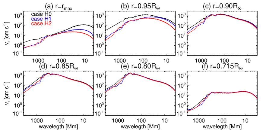
Figure 11: Spectra of the radial velocity at (a) $r=r_{\mathrm{max}}$, (b) $r=0.95R_{\odot}$, (c) $r=0.90R_{\odot}$, (d) $r=0.85R_{\odot}$, (e) $r=0.80R_{\odot}$, (f) $r=0.715R_{\odot}$. The black, blue, and red lines specify the results in cases H0, H1, and H2, respectively.

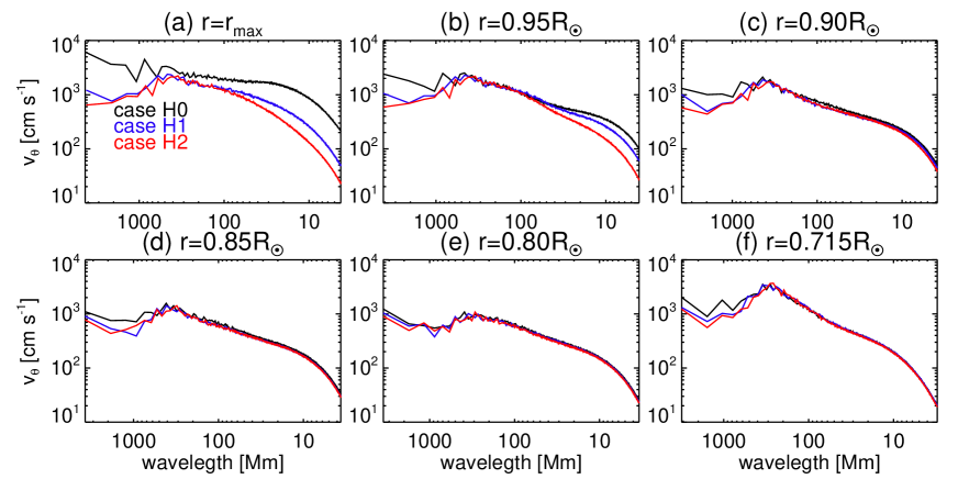
Figure 12: Spectra of the latitudinal velocity at (a) $r=r_{\mathrm{max}}$, (b) $r=0.95R_{\odot}$, (c) $r=0.90R_{\odot}$, (d) $r=0.85R_{\odot}$, (e) $r=0.80R_{\odot}$, (f) $r=0.715R_{\odot}$. The black, blue, and red lines specify the results in cases H0, H1, and H2, respectively.

Figs. 11 and 12 show the spectra of the radial velocity ($v_{r}$) and the latitudinal velocity ($v_{\theta}$), respectively, as a function of the horizontal wavelength ($L_{\mathrm{h}}=2\pi r/l$), where $l$ is the spherical harmonic degree, i.e., the horizontal wavenumber. The black, blue, and red lines show the results in case H0 ($r_{\mathrm{max}}=0.99R_{\odot}$ and $d_{\mathrm{c}}=3740\ \mathrm{km}$), H1 ($r_{\mathrm{max}}=0.96R_{\odot}$ and $d_{\mathrm{c}}=3740\ \mathrm{km}$), and H2 ($r_{\mathrm{max}}=0.96R_{\odot}$ and $d_{\mathrm{c}}=18780\ \mathrm{km}$), respectively. The black line in Fig. 11a shows a peak around $L_{\mathrm{h}}\sim 7$-$8\ \mathrm{Mm}$ (see also Fig. 4). This peak moves to the larger scale $L_{\mathrm{h}}$ with increasing depth. At $r=0.80R_{\odot}$, the peak is around $L_{\mathrm{h}}\sim 300\ \mathrm{Mm}$ (Fig. 11f, black line). This reflects the variation of the pressure scale height in the solar model, $H_{p}=1.9\ \mathrm{Mm}$ at $r=0.99R_{\odot}$ and $H_{p}=44\ \mathrm{Mm}$ at $r=0.8R_{\odot}$ (see Fig. 1e). Again the peak is in the smaller scale ($\sim 7\ \mathrm{Mm}$) at the bottom boundary $r=r_{\mathrm{min}}=0.715R_{\odot}$. This is caused by the collision between the downflow and the impenetrable bottom boundary. In this process a thin boundary layer whose thickness is determined by the numerical resolution is formed. The scale of turbulence near the boundary (Fig. 11f) is a consequence of this boundary layer. A comparison of black lines in Fig. 11a and 12a indicates that the peak of the latitudinal velocity is at a much larger scale ($\sim 400\ \mathrm{Mm}$) than the radial velocity, even close to the upper boundary. We note that almost all the spectra have this feature around $L_{\mathrm{h}}\sim 400\ \mathrm{Mm}$, i.e., the peak or the bended feature in which the power-law index varies. The length of the scale $400\ \mathrm{Mm}$ is twice the thickness of the convection zone, i.e., the radial extent of our computational domain. This result is consistent with our previous study (Hotta et al. 2012a), which argues that the typical scale of the convection is determined by the pressure (or density) scale height or the height of the computational domain. Fig. 12a shows that the horizontal velocity is more likely to be influenced by the large scale structure.

The influences from the location of the boundary and the thickness of the cooling layer are discussed by comparing the black, blue and red lines in Figs. 11 and 12. The common feature is that the spectra do not depend on these two factors in the deep layer ($r\leq 0.85R_{\odot}$:panels d, e, and f). This suggests that the small-scale convection caused by the short pressure scale height or the thin cooling layer cannot influence the convection in the deeper region. On the top boundary (Figs. 11a and 12a), the small-scale convection is suppressed gradually from case H0 to H2. This is confirmation of our understanding from the appearance of the convection pattern in §4.1. In the near-surface layer ($r=0.95R_{\odot}$), the difference still remains unchanged. Moving the location of the top boundary upward increases the amplitude of the fluid velocity at all scales (black line). Reducing the thickness of the cooling layer while keeping the location of the boundary unchanged leads to an increase of velocity on small scales (¡50 Mm), while larger scales are unaffected (blue line). We point out that when the surface layer ($0.96R_{\odot}<r<0.99R_{\odot}$) is included, the spectrum of the latitudinal velocity ($v_{\theta}$) is flat from the middle to the small scale ($10<L_{\mathrm{h}}<40$ Mm in Fig. 12b). This is caused by the penetration of the corresponding-scale plume from the near-surface layer.

4.4 Analysis using spherical harmonics and the probability density function for the magnetohydrodynamic cases

In this subsection, we analyze the results of the magnetohydrodynamic calculation in cases M0, M1, and M2 using spherical harmonics and probability density function. We note that cases M0, M1, and M2 use the same parameters as cases H0, H1, and H2, respectively, with the magnetic field. We focus on the influence of the location of the boundary layer and the thickness of the cooling layer on the structure of the magnetic field.

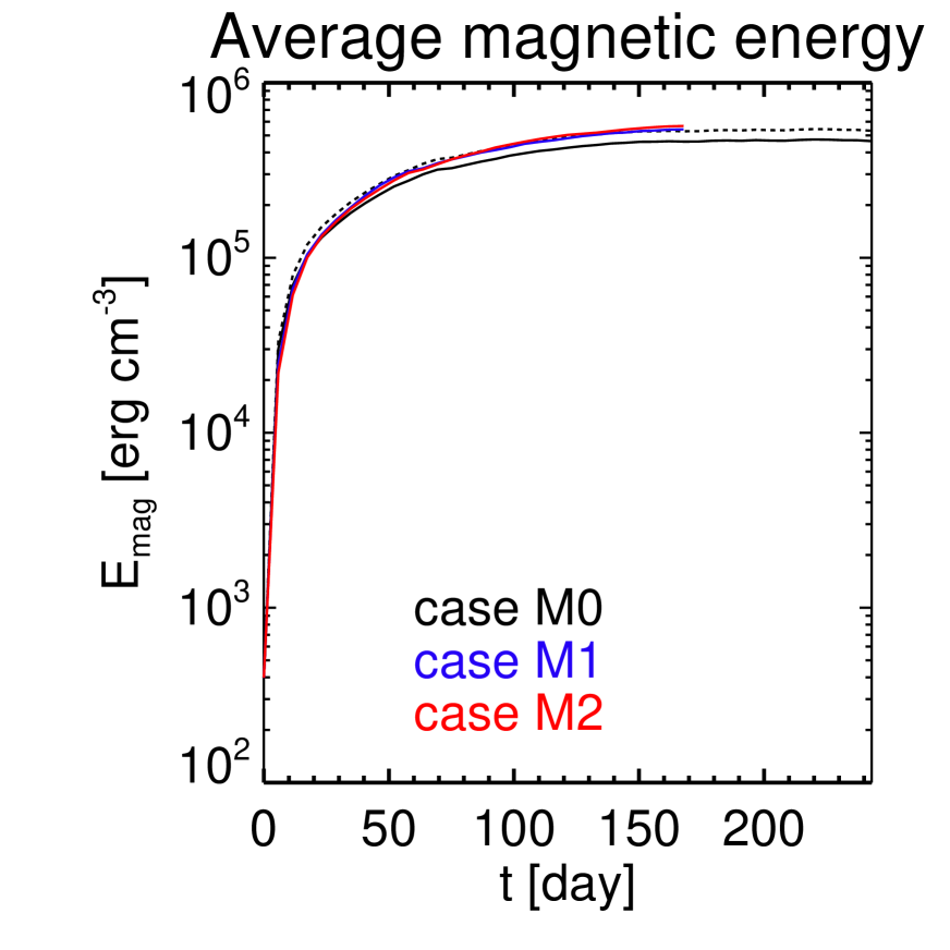
Figure 13: The time evolution of the average magnetic energy is shown. The black, blue and red lines show the results in cases M0, M1 and M2, respectively. The dashed line shows the magnetic energy in case M0 averaged over $r_{\mathrm{min}}<r<0.96R_{\odot}$. $t=0$ is time at which the magnetic field is imposed.

Fig. 13 shows the time evolution of the magnetic energy ($B^{2}/(8\pi)$) averaged over the simulation domain at each time step. The initial linear growth stops around 10 days after the input of the seed field in every case. Even after that the magnetic energy continues to increase gradually with a rather small growth rate until it saturates after around 150 days in all cases. A comparison among the cases is performed using the data from $t=115\ \mathrm{day}$ to $t=162\ \mathrm{day}$ in which the generation of the magnetic field is almost saturated. Basically, the differences among the cases are insignificant, although case M0 saturates with a slightly smaller average magnetic energy. Since the equipartition magnetic field strength in the near-surface region is smaller due to the small density ($\rho_{0}$), the increase of the volume in case M0 causes the slight decrease in the average magnetic energy. This conclusion can be supported by the fact that the average value over $r_{\mathrm{min}}<r<0.96R_{\odot}$ in M0 is larger, as shown by the dashed line in Fig. 13. The growth rate of this energy (dashed line) is higher than those in M1 and M2 at $t<50$ days. The time scale of the convection in the near-surface layer is short. The generated magnetic field is transported downward (see also the discussion about the pumping in §4.5).

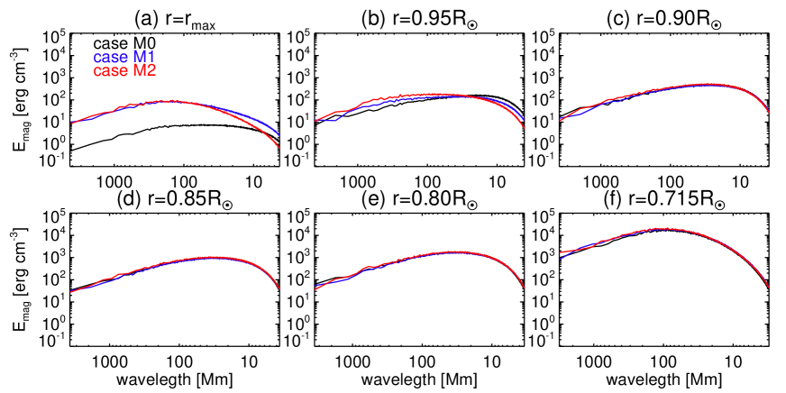
Figure 14: Spectra of the magnetic energy ($B^{2}/8\pi$) at (a) $r=r_{\mathrm{max}}$, (b) $r=0.95R_{\odot}$, (c) $r=0.90R_{\odot}$, (d) $r=0.85R_{\odot}$, (e) $r=0.80R_{\odot}$, (f) $r=0.715R_{\odot}$. The black, blue, and red lines specify the results in cases M0, M1, and M2, respectively.

Fig. 14 shows the spectra of the magnetic energy $B^{2}/(8\pi)$ at selected depths. Similar to the results introduced in the previous sections, the differences can be seen in the near-surface layer, and these differences become insignificant as we go to the deeper layers.

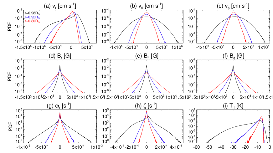
Figure 15: The probability density function of (a) the radial velocity, (b) the latitudinal velocity, (c) the longitudinal velocity, (d) the radial magnetic field, (e) the latitudinal magnetic field, (f) the longitudinal magnetic field, (g) the radial vorticity, (h) the horizontal divergence, and (i) the temperature perturbation are shown using the results in case M0 at $t=115\ \mathrm{day}$.

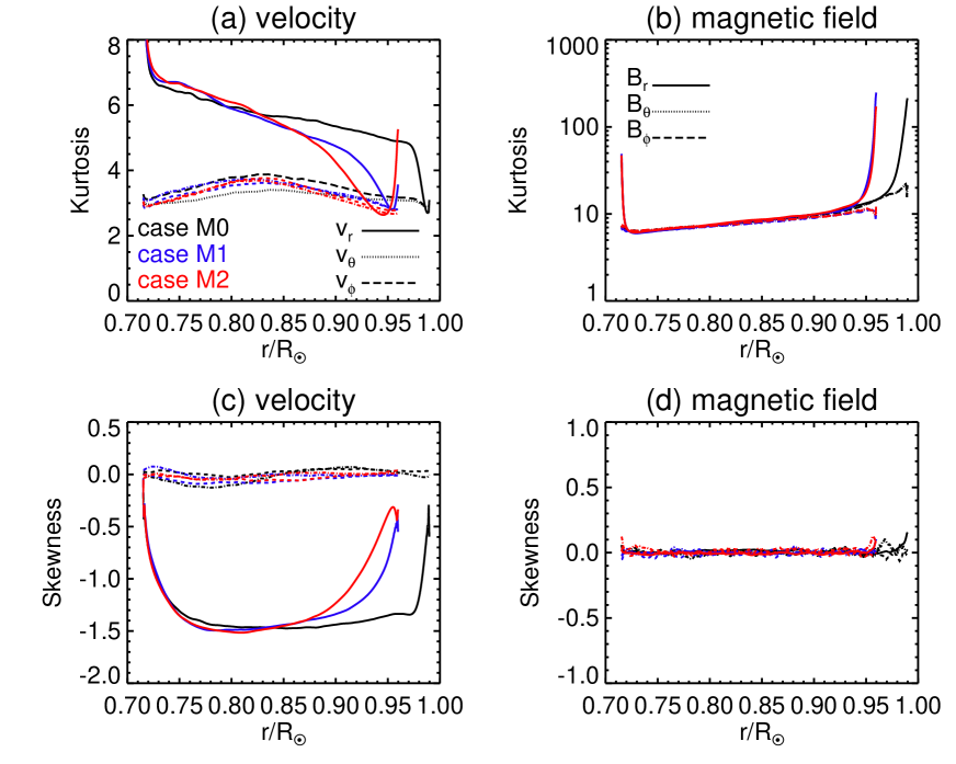
Figure 16: The kurtosis (the fourth central moment of the PDF defined in eq. (24):a and b) and the skewness (the third central moment of the PDF defined in eq. (25):c and d) for the three components of velocity and magnetic field are shown. The black, blue and red lines show the results in cases M0, M1, and M2.

Fig. 15 shows the probability density functions (PDFs) for the three components of velocity ($v_{r}$, $v_{\theta}$, and $v_{\phi}$) and the three components of the magnetic field ($B_{r}$, $B_{\theta}$, and $B_{\phi}$), the radial vorticity $\omega_{r}$, the horizontal divergence $\zeta$ and the temperature perturbation $T_{1}$ in case M0 at $t=115\ \mathrm{day}$. Although the rotation is not included in this study, some features of the PDFs are similar to findings from previous studies including rotation (Brun et al. 2004; Miesch et al. 2008). In this study, the PDF is the normalized histogram on a horizontal surface, corrected for the grid convergence at the poles. Fig. 15a shows the significant asymmetry in the radial velocity. This reflects the asymmetry between up- and downflows due to stratification (see also Figs. 8 and 10). The horizontal velocities ($v_{\theta}$ and $v_{\phi}$) almost show a Gaussian distribution (see also Fig. 16). The magnetic fields have high intermittency compared with the velocities (Brandenburg et al. 1996). Despite our asymmetric initial condition for the longitudinal magnetic field $B_{\phi}=100\ \mathrm{G}$, the PDFs show a close to symmetric distribution peaked at zero after a sufficiently long temporal evolution. The maximum value of the strength of the magnetic field is around $10^{4}\ \mathrm{G}$. The PDF for the radial vorticity is similar to that of the magnetic field, i.e., with high intermittency. This can be expected based on the similarity between the induction and vorticity equations. The horizontal divergence has similarity to the radial vorticity $\omega_{r}$ in the convection zone with high intermittency, while $\zeta$ shows the asymmetry near the top boundary is similar to the radial velocity $v_{r}$. The temperature perturbation has significant asymmetry, which also reflects the asymmetry between the upflow and downflow.

In order to evaluate the influence of the location of the boundary condition and the thickness of the cooling layer, we investigate the moments of the PDF, in particular the kurtosis $\mathcal{K}$ and the skewness $\mathcal{S}$ as

$$\mathcal{K}=\frac{1}{\sigma^{4}}\int(x-\langle x\rangle)^{4}f(x)dx,$$ (24)

$$\mathcal{S}=\frac{1}{\sigma^{3}}\int(x-\langle x\rangle)^{3}f(x)dx,$$ (25)

where $f(x)$ is the PDF, $x$ is each variable, and $\sigma$ is the standard deviation as

$$\sigma=\sqrt{\int(x-\langle x\rangle)^{2}f(x)dx}.$$ (26)

The kurtosis $\mathcal{K}$ and the skewness $\mathcal{S}$ denote the intermittency and the asymmetry of the distribution, respectively. We note that the PDF is normalized as $\int f(x)dx=1$. For example the Gaussian PDF is characterized by $\mathcal{K}=3$ and $\mathcal{S}=0$. Fig. 16 shows the distribution of the kurtosis and the skewness for the velocity and the magnetic field. As noted above, the horizontal velocities ($v_{r}$ and $v_{\phi}$) have almost a Gaussian distribution, i.e., $\mathcal{K}\sim 3$ and $\mathcal{S}\sim 0$ throughout the convection zone. The radial velocity has high intermittency and asymmetry in the convection zone. The magnetic field has intermittency and almost symmetric distribution. These features are common among cases M0, M1, and M2. Quantitatively the kurtosis and skewness agree with each other in all cases. While the values in the near-surface region ($r>0.85R_{\odot}$) are influenced by the two factors considered, the location of the upper boundary and the thickness of the cooling layer, in the deeper region the values converge.

4.5 Generation and transportation of the magnetic field

In this subsection we investigate the generation and transport of the magnetic field by turbulent thermal convection. The global structure of the mutual interaction between the plasma and the magnetic field is our paramount interest.

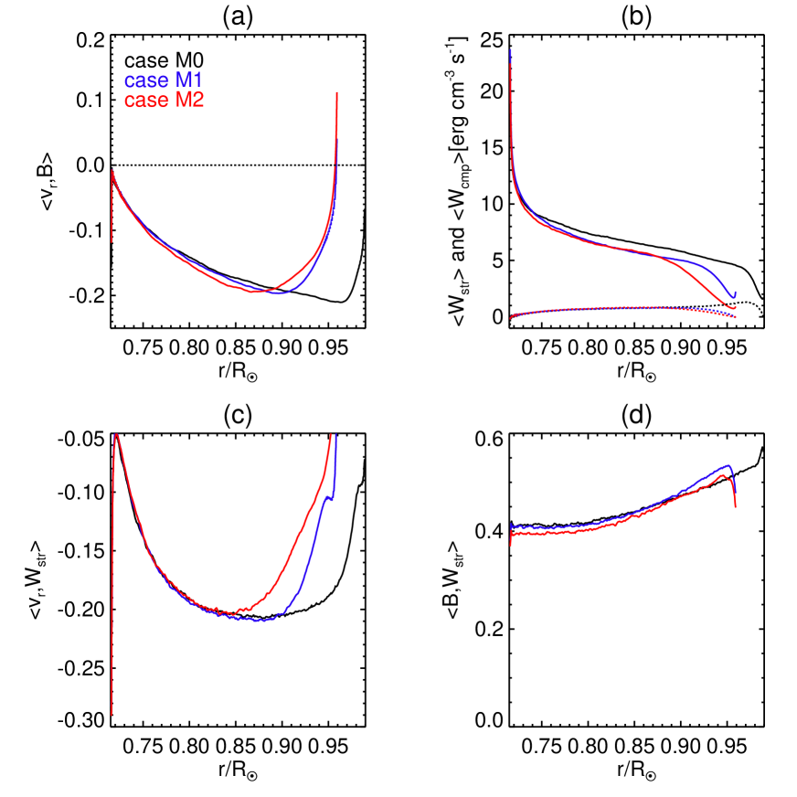
Figure 17: (a) The correlation between the radial velocity and the strength of the magnetic field ($\langle v_{r},B\rangle$), (b) the horizontal average of the generation rate of the magnetic energy by the stretching ($\langle W_{\mathrm{str}}\rangle$: solid line) and the compression ($\langle W_{\mathrm{cmp}}\rangle$: dashed line), (c) the correlation between the radial velocity and the generation rate of the magnetic energy ($\langle v_{r},W_{\mathrm{str}}\rangle$), (d) the correlation between the strength of the magnetic field and the generation rate of the magnetic energy ($\langle B,W_{\mathrm{str}}\rangle$) are shown.

Fig. 6 shows the radial velocity $v_{r}$, the radial magnetic field $B_{r}$, and the radial vorticity $\omega_{r}$ at different depths ($r=0.99R_{\odot}$:a, b, and c, $r=0.95R_{\odot}$:d, e, and f, $r=0.85R_{\odot}$:g, h, and i). As introduced in §4.1, there is good coincidence between the downflow and regions with a large amplitude of the radial vorticity. This means that downflows, especially in the deeper region, include most of the turbulent small-scale horizontal motions. We can also see the preferential association of a strong magnetic field with downflows and regions with strong vorticity in the constant-depth plane (middle and right columns of Fig. 6) and also in the meridional plane (Fig. 7). In order to investigate this aspect quantitatively, we estimate the correlation between the radial velocity $v_{r}$ and the absolute value of the magnetic field $B$, i.e., $\langle v_{r},B\rangle$ in Fig 17a where our definition of the correlation between quantity $A$ and $B$ is defined as:

$$\langle A,B\rangle=\frac{\int ABdS}{\sqrt{\int A^{2}dS}\sqrt{\int B^{2}dS}}.$$ (27)

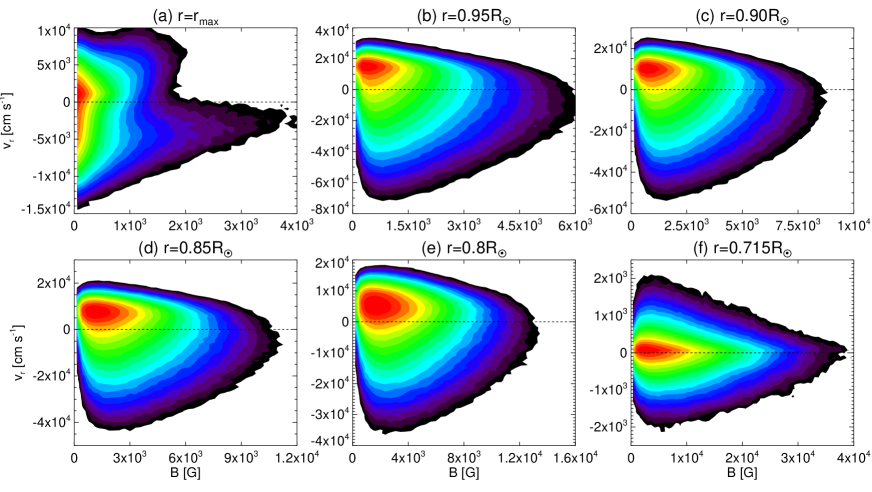
Figure 18: Joint PDFs with the radial velocity ($v_{r}$) and the strength of the magnetic field ($B$) in the case M0 at (a) $r=r_{\mathrm{max}}$, (b) $r=0.95R_{\odot}$, (c) $r=0.90R_{\odot}$, (d) $r=0.85R_{\odot}$, (e) $r=0.80R_{\odot}$, (f) $r=r_{\mathrm{min}}=0.715R_{\odot}$. The black lines show $v_{r}=0$, which distinguish the upflow and the downflow.

Fig. 17a shows the negative value in most of the convection zone. This means that the magnetic field is preferentially found in downflows. This is also seen in the joint PDFs of $v_{r}$ and $B$ in Fig. 18. The figure shows the asymmetric distribution about the $v_{r}=0$ axis in the convection zone. A strong magnetic field is more likely to be located in downflow regions. We note that a symmetric distribution is found at $r=r_{\mathrm{min}}$, which corresponds to $\langle v_{r},B\rangle\sim 0$ in Fig. 17a.

There are two possibilities for the preference of the magnetic field to downflow regions. One is that the magnetic field is generated uniformly in space and transported to the downflow region by converging motion. The other is that the magnetic field is generated in the downflow region. In order to answer this question, we define and evaluate the generation rate of magnetic energy by the stretching ($W_{\mathrm{str}}$) and the compression ($W_{\mathrm{cmp}}$) as:

$$W_{\mathrm{str}}=\frac{\bf B}{4\pi}\cdot\left[(\bf B\cdot\nabla)\bf v\right],$$ (28)

$$W_{\mathrm{cmp}}=-\frac{B^{2}}{4\pi}(\nabla\cdot{\bf v}).$$ (29)

The estimations for the horizontal averages, $\langle W_{\mathrm{str}}\rangle$ and $\langle W_{\mathrm{cmp}}\rangle$, are shown in Fig 17b. It is clear that the value of the stretching $\langle W_{\mathrm{str}}\rangle$ is much larger than that of the compression throughout the convection zone and that the generation of the magnetic field is basically done by the stretching in the turbulent motion. This is also seen by the realistic calculations in the photosphere (Pietarila Graham et al. 2010), which suggest that 95% of the gain of the magnetic energy is done by the stretching. We also estimate the correlation between the radial velocity $v_{r}$ and the energy generation rate by the stretching $W_{\mathrm{str}}$ (Fig. 17c). The distribution of this correlation is similar to that of $\langle v_{r},B\rangle$, i.e., the effective stretching prefers the downflow region. Thus we conclude that the reason the strong magnetic field prefers the downflow region is that the magnetic field is more likely to be generated there. The correlation between $B$ and $W_{\mathrm{str}}$ is also estimated. This shows a larger value of ($>0.4$) throughout the convection zone (Fig. 17d). The features discussed above are basically common among the studied cases.

In order to investigate magnetic field transport in the convection zone, we evaluate the Poynting flux given by:

$$F_{\mathrm{m}}=\frac{c}{4\pi}\left(E_{\theta}B_{\phi}-E_{\phi}B_{\theta}\right),$$ (30)

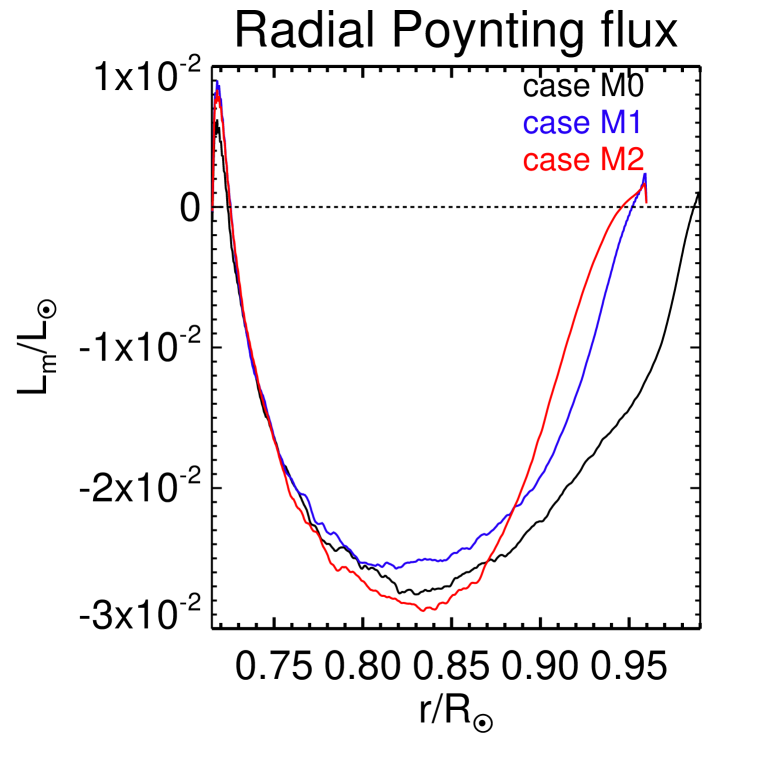
Figure 19: The integrated radial Poynting flux as a function of the depth is shown. The black, blue and red lines show the results in cases M0, M1, and M2, respectively.

where the electric field is defined as ${\bf E}=-({\bf v}\times{\bf B})/c$ and $c$ is the speed of light (see Brun et al. (2004)). Fig. 19 shows the horizontally integrated Poynting flux $L_{\mathrm{m}}$ as a function of the depth. Since the absolute value ($\sim 10^{31}\ \mathrm{erg\ s^{-1}}$) is much smaller than the solar luminosity ($L_{\odot}=3.84\times 10^{33}\ \mathrm{erg\ s^{-1}}$), the Poynting flux does not contribute significantly to the total energy flux balance. The Poynting flux is negative in most of the convection zone, since a strong magnetic field is concentrated in downflow regions. This is suggested by previous studies as the turbulent pumping effect (see, e.g., Tobias et al. 1998, 2001). Within the convection zone, the flux has a positive value only in the thin layer ($\sim 0.01R_{\odot}$) close to the bottom. This is caused by the bounced motion from the bottom boundary. The magnetic energy is transported upward, causing the magnetic flux in the upflow region. This can be one of the reasons why the absolute values of the correlation $\langle v_{r},B\rangle$ is small in the deeper region (Fig. 17a) and why the distribution of the joint PDF in the bottom (Fig. 18f) is symmetric.

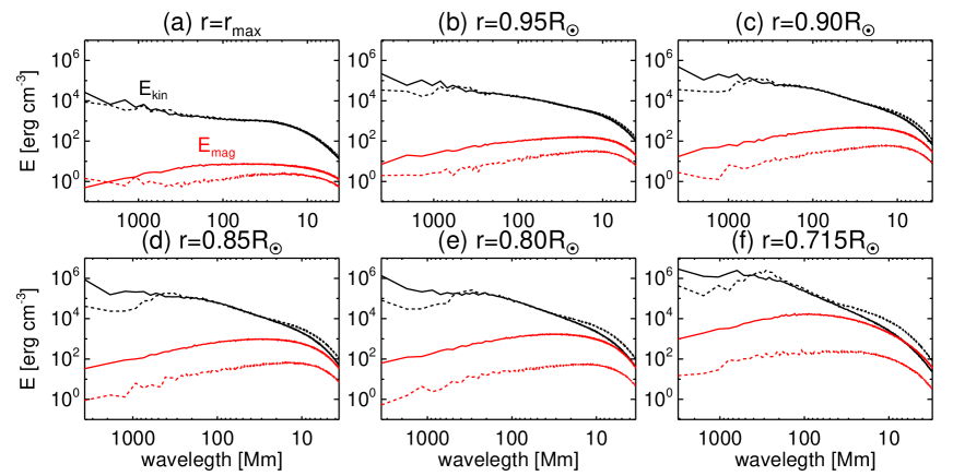
Figure 20: The spectra of the kinetic energy ($E_{\mathrm{kin}}=\rho_{0}v^{2}/2$: solid black lines) and the magnetic energy ($E_{\mathrm{mag}}=B^{2}/(8\pi)$: solid red lines) in case M0. The dashed black lines show the kinetic energy in H0, i.e., without the magnetic field. The dashed red lines show the magnetic energy at $t=5.8$ days.

In the following discussion, we investigate the scale of the magnetic field generated. Fig. 20 shows the spectra of the kinetic energy (black lines: $E_{\mathrm{kin}}=\rho_{0}v^{2}/2$) and the magnetic energy (red lines: $E_{\mathrm{mag}}=B^{2}/(8\pi)$) in case M0 averaged from $t=173\ \mathrm{day}$ to $t=237\ \mathrm{day}$ in which the generation of the magnetic field is close to being saturated. The dashed black and red lines show the kinetic energy without the magnetic field and the magnetic energy at $t=5.8$ days, respectively. In the upper convection zone ($\geq 0.85R_{\odot}$), the spectra of the magnetic energy peaks at the smallest scale, which is typical for the kinematic phase of a local dynamo. Finding this feature in the saturated phase indicates that the local dynamo is likely not very efficient for our resolved scales ($>7\ \mathrm{Mm}$). We see also no indication that the kinetic energy spectrum changed due to the presence of the dynamo near the top of the domain. This situation is different in the lower half of the domain. Figs. 20e and f show some peak shift of the magnetic energy to larger scales and some feedback on thermal convection, i.e., the kinetic energy is suppressed on the smallest scales. Here the magnetic energy slightly exceeds the kinetic energy near the smallest scales. This shows that a more efficient local dynamo can be achieved to some extent for our resolution in the lower part of the convection zone ($<0.85R_{\odot}$).

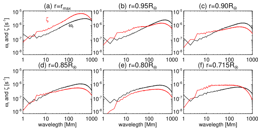
Figure 21: The spectra of the horizontal divergence $\zeta$ and the radial vorticity $\omega_{r}$ using the result in case M0.

Fig. 21 shows that the spectra of the horizontal divergence ($\zeta$) and the radial vorticity ($\omega_{r}$) show a similar distribution to that of the magnetic field with the peak at small scales. Moffatt (1961) suggested that the power spectrum varies as $D_{b}(k)\propto k^{2}D_{v}(k)$ when the magnetic field is proportional to $(\nabla\cdot{\bf v})$ or $(\nabla\times{\bf v})$, where $D_{b}(k)$ and $D_{v}(k)$ are magnetic and kinetic spectra. This was recently confirmed through solar observations in the photosphere using the Hinode satellite (Katsukawa & Orozco Suárez 2012). Since in our calculation there is similarity between the magnetic field and the vorticity or the divergence, the magnetic energy peaks at smaller scales than does the kinetic energy. We note that differences can be seen between the shear of the velocity ($\omega_{r}$ and $\zeta$) and the magnetic energy ($E_{\mathrm{mag}}$) at the base of the convection zone (Fig. 20f and 21f), where the feedback from the magnetic field is stronger.

Even though the numerical resolution does not vary much with depth, the effectiveness of the local dynamo is not expected to be depth independent. There are two reasons for this: The intrinsic convective scale varies with depth, and a downward Poynting flux exists almost everywhere in the convection zone. In the upper half of the convection zone the divergence of the Poynting flux provides an energy sink, while at the same time the dynamo is not very efficient on the resolved scale (similar discussion can be found in Stein et al. 2003). In the lower convection zone ($<0.85R_{\odot}$), the radial gradient of the Poynting flux is negative, thus the magnetic energy is accumulated. At the same time the intrinsic scale of convection is larger and better resolved, leading to a more efficient dynamo. It should be noted that Vögler & Schüssler (2007) found that even in near-surface areas the small-scale convection reproduced with high resolution has a time scale short enough to amplify the magnetic field against the pumping effect.

In order to confirm our idea about the generation and transportation of the magnetic field in our calculation, we evaluate the effective shear for the magnetic field,

$$f_{\mathrm{eff}}=\frac{\langle W_{\mathrm{str}}\rangle}{\langle B^{2}/(8\pi)\rangle}.$$ (31)

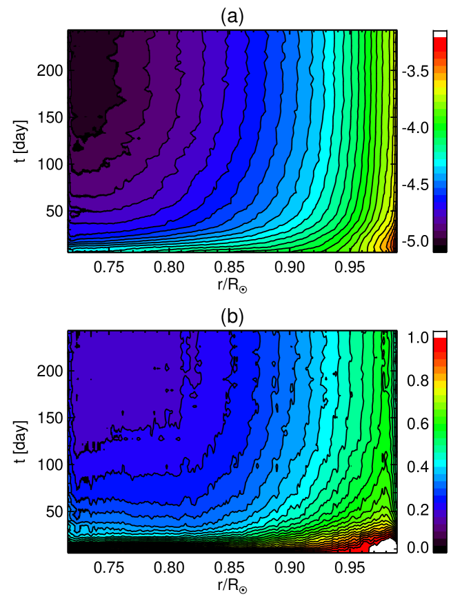
Figure 22: The time evolution of the effective shear (a) $\log f_{\mathrm{eff}}$ and (b) $f_{\mathrm{eff}}(t)/f_{\mathrm{eff}}(t=5.8\ \mathrm{day})$.

$f_{\mathrm{eff}}$ has the unit of $\mathrm{s^{-1}}$ and indicates the time scale of the amplification. Fig. 22a shows the time evolution of $\log f_{\mathrm{eff}}$ and indicates that regardless of the phase of the generation of the magnetic field, the larger value of $f_{\mathrm{eff}}$ is seen in the upper convection, which reflects the short time scale of the thermal convection there. At later times with a stronger magnetic field, the effective shear $f_{\mathrm{eff}}$ is reduced, and after $t\sim 150$, it remains constant. Fig. 22b shows the ratio to the value at $t=5.8\ \mathrm{day}$, i.e. $f_{\mathrm{eff}}(t)/f_{\mathrm{eff}}(t=5.8\ \mathrm{day})$. The suppression of the effective shear depends on the depth. It is more suppressed in the deeper region. This might be caused by the feedback of the magnetic field on the velocity seen in Fig. 20 (the solid and dashed black lines) as well as a misalignment between the shear and magnetic field around the base of the convection zone. The ineffective suppression of $f_{\mathrm{eff}}$ in the upper convection zone confirms our idea presented in the previous paragraph. The local dynamo saturates there with little non-linear feedback (suppression of $f_{\mathrm{eff}}$), since the pumping effect works well in the upper region and the dynamo is not very efficient on the resolved scales to begin with.

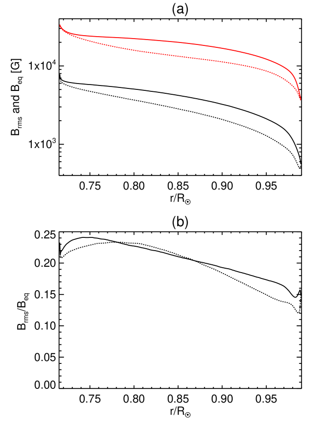
Figure 23: (a) The distribution of the equipartition field $B_{\mathrm{eq}}$ (red lines) and the RMS magnetic field $B_{\mathrm{rms}}$ (black lines). (b) The ratio of the RMS magnetic field and the equipartition magnetic field ($B_{\mathrm{rms}}/B_{\mathrm{eq}}$). The solid and dashed lines show the values at the downflow and the upflow regions, respectively.

Fig. 23 also shows the variation of dynamo efficiency in the convection zone. Fig. 23a shows the equipartition magnetic field $B_{\mathrm{eq}}=\sqrt{4\pi v_{\mathrm{rms}}^{2}}$ and the RMS magnetic field $B_{\mathrm{rms}}$ as functions of the depth. The solid and dotted lines show the values at the downflow and upflow regions, respectively. Basically, both $B_{\mathrm{eq}}$ and $B_{\mathrm{rms}}$ increase with the depth and, Fig. 23b shows an increase of $B_{\mathrm{rms}}/B_{\mathrm{eq}}$ with depth, which is caused by the ineffectiveness of the local dynamo in the upper region due to the pumping effect and our insufficient resolution.

5 Discussion and Summary

We carry out the high-resolution calculations of the solar global convection which resolve 10 Mm-scale convection smaller than the supergranulation using the RSST (described in §2). The RSST leads to a simple algorithm and requires only local communication in the parallel computing. In addition, this method has the capability to access the real solar surface without undermining the important physics. This enables us to capture near-surface small-scale convection while keeping a global domain. Our main conclusions are given as follows: 1. Small-scale convection is excited close to the surface ($>0.9R_{\odot}$), when we expand our domain upward to $0.99\,R_{\odot}$ to capture the near-surface layers with small pressure scale heights. 2. In deeper convection zones ($<0.9R_{\odot}$), the convection flow is not influenced by the location of the top boundary and the assumed thickness of the thermal boundary layer. Changing the position of the top boundary or thickness of the cooling layer does not lead to significant differences in the convective structure and properties of the local dynamo, in terms of the power-spectrum, the probability density function and the local dynamo. 3. Using an LES approach we can achieve small-scale dynamo action and maintain a field of about $0.15-0.25B_{\mathrm{eq}}$ throughout the convection zone. 4. The overall dynamo efficiency varies significantly in the convection zone as a consequence of the downward directed Poynting flux and the depth variation of the intrinsic convective scales. For a fixed numerical resolution, the dynamo-relevant scales are better resolved in the deeper convection zone and are therefore less affected by numerical diffusivity, i.e., the effective Reynolds numbers are larger.

Recently, Hanasoge et al. (2012) suggested that there is a significant difference between the calculation by Miesch et al. (2008) and flow velocities inferred from local helioseismology. The observed convection amplitude is much smaller than that in the hydrodynamic calculation. We expected that the modification to the location of the upper boundary may help to resolve this issue. Conclusion 1 above, however, suggests that the difference between the calculation and the observation becomes larger when we move the top boundary further upward. We see, nevertheless, some indication that the kinetic energy is reduced on the largest scales when a local dynamo is present. At the same time, we cannot fully rule out the possibility that unresolved small-scale turbulence near the top boundary contributes to this issue, since the intrinsic scale of the convection near our top boundary is still not well resolved.

Conclusion 2 is one of the most important results in this study, since it suggests that previous calculations such as by Miesch et al. (2008) are physically reasonable in the deeper convection zone even if the top boundary condition is placed significantly below the solar surface.

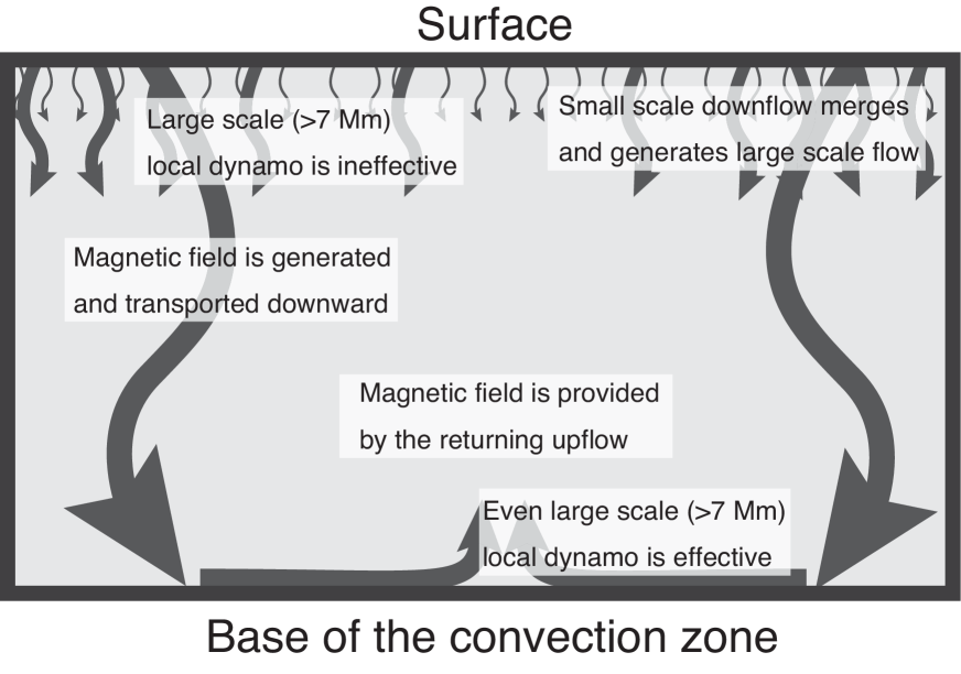
Figure 24: The schematic view of our calculation. The arrows show the convection flow. The conclusion that the dynamo is ineffective near the top is based on the comparison of the kinematic and saturated spectra and the only moderate reduction of the effective shear in the upper convection zone (see §4.5).

We summarize our simulation results in a schematic picture shown in Fig. 24. The conclusion that the dynamo is ineffective near the top comes from the comparison of the kinematic and saturated spectra and the only moderate reduction of the effective shear in the upper convection zone (see §4.5). Since several aspects, in particular with regard to the local dynamo, require higher resolution before being directly applicable to the solar convection zone, Fig. 24 does not necessarily apply to the real Sun. High resolution simulations of a local dynamo in the solar photosphere (Vögler & Schüssler 2007) suggest that efficient dynamo action is possible even in the presence of the pumping effect. These simulations use, however, a grid resolution of about a factor of $100$ larger than our setup, which is currently inapplicable for global scale convection simulations. Therefore, the dynamo RMS field strength of $0.15-0.25B_{\mathrm{eq}}$ can likely be considered a lower limit.

One issue we cannot address in this study is the problem regarding the small magnetic Prandtl number ($\mathrm{Pm}\sim 10^{-3}$) in the solar convection zone, since we adopt numerical diffusivities which assume that the magnetic Prandtl number is around unity. Several authors argued that smaller magnetic Prandtl numbers make local dynamos less efficient (e.g. Schekochihin et al. 2004; Boldyrev & Cattaneo 2004). In other words, a small magnetic Prandtl number requires a larger magnetic Reynolds number in order to achieve a super-critical dynamo. While this can be a significant problem for numerical simulations with rather moderate Reynolds numbers, this is less likely an issue in the solar convection zone with Reynolds numbers as large as $\mathrm{Rm}\sim 10^{11}$ (Brandenburg 2011). Thus we believe that our approach relying only on numerical diffusivities can capture the physics of the local dynamo in the solar convection zone.

Rotation is not included in this study although it plays a key role in organizing large-scale flows and enabling large-scale dynamo action. Studying the near-surface small-scale convection in a setup with rotation is of particular interest to us for investigation of the origin of the near-surface shear layer observed on the Sun. Our investigation of this is a work-in-progress and will be presented in a forthcoming paper. Further progress can be made by using non-uniform grids, such as nested grids or adaptive mesh refinement, which are useful in order to overcome the significant differences in spatial and temporal dynamic scales. These methods are already implemented in our numerical code (Hotta & Yokoyama 2012).

Appendix A Equation of state in the solar convection zone

In the numerical simulations of the convection in the near-surface layer, the ordinary tabular equation of state is widely used (Vögler et al. 2005; Rempel et al. 2009). However, this is not a viable approach for our current simulations, since the deviations from the reference state are small, e.g., $\rho_{1}/\rho_{0}\sim 10^{-6}$ around the base of the convection zone. Thus we adopt another way to treat the ionization effect in the near-surface layer. The fluctuations from the reference state are calculated as:

$$p_{1}=\left(\frac{\partial p}{\partial\rho}\right)_{s}\rho_{1}+\left(\frac{\partial p}{\partial s}\right)_{\rho}s_{1},$$ (A1)

$$T_{1}=\left(\frac{\partial T}{\partial\rho}\right)_{p}\rho_{1}+\left(\frac{\partial T}{\partial p}\right)_{\rho}p_{1},$$ (A2)

$$e_{1}=\left(\frac{\partial e}{\partial\rho}\right)_{T}\rho_{1}+\left(\frac{\partial e}{\partial T}\right)_{\rho}T_{1}.$$ (A3)

The first derivatives, such as $(\partial p/\partial\rho)_{s}$, are described by the background variables, $\rho_{0}(r)$, $p_{0}(r)$… and are regarded as functions of the depth $r$. In the OPAL routine (Rogers et al. 1996), the values $(\partial e/\partial\rho)_{T}$, $(\partial e/\partial T)_{\rho}$, $(\partial p/\log\rho)_{T}$ and $(\partial p/\log T)_{\rho}$ are provided for given $\rho_{0}$, $T_{0}$, and the mass fraction of hydrogen ($X$), helium ($Y$) and other metals ($Z$). We show the relations between the OPAL-provided variable and the required variable derived from the first law of thermodynamics (Mihalas & Mihalas 1984).

$$\left(\frac{\partial p}{\partial\rho}\right)_{s}=\frac{c_{\mathrm{p}}}{\kappa_{\mathrm{t}}\rho_{0}c_{\mathrm{v}}},$$ (A4)

$$\left(\frac{\partial p}{\partial s}\right)_{\rho}=\frac{\beta_{\mathrm{p}}T_{0}}{\kappa_{\mathrm{t}}c_{\mathrm{v}}},$$ (A5)

$$\left(\frac{\partial T}{\partial\rho}\right)_{p}=-\frac{1}{\rho_{0}\beta_{\mathrm{p}}},$$ (A6)

$$\left(\frac{\partial T}{\partial p}\right)_{\rho}=T_{0}/\left(\frac{\partial p}{\partial\log T}\right)_{\rho},$$ (A7)

where $\beta_{p}$, $c_{\mathrm{v}}$, $c_{\mathrm{p}}$ and $\kappa_{\mathrm{t}}$ are the coefficient of thermal expansion, the specific heat at constant volume and pressure, the coefficient of isothermal compressibility, respectively, defined as:

$$\beta_{\mathrm{p}}\equiv-\left(\frac{\partial\log\rho}{\partial T}\right)_{p}=\frac{1}{T_{0}}\left(\frac{\partial p}{\partial\log T}\right)_{\rho}/\left(\frac{\partial p}{\partial\log\rho}\right)_{T},$$ (A8)

$$c_{\mathrm{v}}=\left(\frac{\partial e}{\partial T}\right)_{\rho},$$ (A9)

$$c_{\mathrm{p}}=c_{\mathrm{v}}-T_{0}\beta_{\mathrm{p}}\left[\left(\frac{\partial e}{\partial\rho}\right)_{T}-\left(\frac{p}{\rho^{2}}\right)\right],$$ (A10)

$$\kappa_{\mathrm{t}}=\left(\frac{\partial\log\rho}{\partial p}\right)_{T}.$$ (A11)

Appendix B Conservation of the total energy in the RSST and first-order enthalpy flux

When the equation of the entropy is given as eq. (5), the total energy is not conserved even mathematically. In this appendix, the deviation in the conservation of the total energy caused by the RSST is introduced. Here , we ignore the magnetic field, the gravity and the radiation for the sake of simplicity. The equation of continuity for RSST is defined as eq. (2). Thus there are two relations as:

$$\frac{D\rho}{Dt} = \frac{\partial\rho}{\partial t}+{\bf v}\cdot\nabla\rho$$ (B1)

$$= -\frac{1}{\xi^{2}}\nabla\cdot(\rho{\bf v})+{\bf v}\cdot\nabla\rho$$

$$= \left(1-\frac{1}{\xi^{2}}\right)\nabla\cdot(\rho{\bf v})-\rho\nabla\cdot{\bf v},$$

and

$$\rho\frac{DA}{Dt} = \rho\frac{\partial A}{\partial t}+\rho{\bf v}\cdot\nabla A$$ (B2)

$$= \frac{\partial}{\partial t}(\rho A)+\nabla\cdot\left(\rho A{\bf v}\right)-A\frac{\partial\rho}{\partial t}-A\nabla\cdot(\rho{\bf v})$$

$$= \frac{\partial}{\partial t}(\rho A)+\nabla\cdot\left(\rho A{\bf v}\right)-A\left(1-\frac{1}{\xi^{2}}\right)\nabla\cdot(\rho{\bf v}).$$

There is deviation from the relation with the original equation of continuity. The deviations are proportional to $(1-1/\xi^{2})\nabla\cdot(\rho{\bf v})$. Therefore the deviation between the conservative form and the primitive form of the equation of motion is

$$\left(1-\frac{1}{\xi^{2}}\right){\bf v}\nabla\cdot\left(\rho{\bf v}\right).$$ (B3)

Then the deviation between the equation of entropy and the conservative form for the total energy is introduced as:

$$\rho T\frac{Ds}{Dt} = \rho\frac{De}{Dt}+\rho p\frac{D}{Dt}\left(\frac{1}{\rho}\right)$$ (B4)

$$= \frac{\partial}{\partial t}\left(\rho e\right)+\nabla\cdot\left(\rho e{\bf v}\right)+p\nabla\cdot{\bf v}$$

$$-\left(e+\frac{p}{\rho}\right)\left(1-\frac{1}{\xi^{2}}\right)\nabla\cdot(\rho{\bf v})$$

$$= Q,$$

where $Q$ includes thermal diffusivity and surface cooling. When we start from the primitive form of the equation of motion, the equation of the kinetic energy is expressed as:

$$\frac{\partial}{\partial t}\left(\frac{1}{2}\rho v^{2}\right)+\nabla\cdot\left(\frac{1}{2}\rho v^{2}{\bf v}\right)=-{\bf v}\cdot\nabla p+\frac{1}{2}v^{2}\left(1-\frac{1}{\xi^{2}}\right)\nabla\cdot(\rho{\bf v}).$$ (B5)

Thus the conservative form for the total energy is expressed as:

$$\frac{\partial}{\partial t}\left(\rho e+\frac{1}{2}\rho v^{2}\right) = -\nabla\cdot\left[\left(\rho e+p+\frac{1}{2}\rho v^{2}\right){\bf v}\right],$$ (B6)

$$+\left(e+\frac{p}{\rho}+\frac{1}{2}v^{2}\right)\left(1-\frac{1}{\xi^{2}}\right)\nabla\cdot(\rho{\bf v})+Q.$$

If the speed of sound is much faster than the fluid velocity, the anelastic approximation $\nabla\cdot(\rho{\bf v})=0$ is well achieved. In our calculations over 200 days, we could not see any coherent trend in the energy.

Appendix C First-order enthalpy flux

We derive the first-order radial enthalpy flux. According to eq. (B6), the original form of the radial enthalpy flux is expressed as:

$$F_{\mathrm{e}}=\left(\rho e+p\right)v_{r}.$$ (C1)

In the statistical steady state, horizontal integration and the time average ensure no net transport of mass along the depth, i.e.,

$$\int_{s}\rho v_{r}dS=0.$$ (C2)

In this study the equation of state for the perfect gas is not adopted, and the form of the enthalpy flux is slightly different from previous studies (e.g. Miesch et al. 2008; Käpylä et al. 2011) in which the enthalpy flux is simply expressed as $F_{\mathrm{e}}=c_{\mathrm{p}}\rho_{0}T_{1}v_{r}$. The integrated radial enthalpy flux is calculated as:

$$L_{\mathrm{e}} = \int_{s}\left(e+\frac{p}{\rho}\right)\rho v_{r}dS$$ (C3)

$$= \int_{s}\left(e+\frac{p_{0}+p_{1}}{\rho_{0}+\rho_{1}}\right)\rho v_{r}dS$$

$$\sim \int_{s}\left[e+\frac{p_{0}+p_{1}}{\rho_{0}}\left(1-\frac{\rho_{1}}{\rho_{0}}\right)\right]\rho v_{r}dS$$

$$\sim \int_{s}\left(e_{1}+\frac{p_{1}}{\rho_{0}}-\frac{p_{0}\rho_{1}}{\rho_{0}^{2}}\right)\rho v_{r}dS$$

$$\sim \int_{s}\left(\rho_{0}e_{1}+p_{1}-\frac{p_{0}\rho_{1}}{\rho_{0}}\right)v_{r}dS.$$

The final line of the equation is then adopted for the enthalpy flux in this study.

Table 1: Important parameters in our studies.

Case	H0	H1	H2
$N_{r}$	512	456	456
$r_{\mathrm{max}}/R_{\odot}$	0.99	0.96	0.96
$\displaystyle{\frac{\rho_{0}(r_{\mathrm{min}})}{\rho_{0}(r_{\mathrm{max}})}}$	613	36	36
$H_{p0}(r_{\mathrm{max}})\ [\mathrm{km}]$	1870	9390	9390
$d_{\mathrm{c}}\ \mathrm{[km]}$	3740	3740	18780

References

- Augustson et al. (2011) Augustson, K., Rast, M., Trampedach, R., & Toomre, J. 2011, Journal of Physics Conference Series, 271, 012070
- Boldyrev & Cattaneo (2004) Boldyrev, S., & Cattaneo, F. 2004, Physical Review Letters, 92, 144501
- Brandenburg (2011) Brandenburg, A. 2011, ApJ, 741, 92
- Brandenburg et al. (1996) Brandenburg, A., Jennings, R. L., Nordlund, Å., Rieutord, M., Stein, R. F., & Tuominen, I. 1996, Journal of Fluid Mechanics, 306, 325
- Brandenburg & Subramanian (2005) Brandenburg, A., & Subramanian, K. 2005, Phys. Rep., 417, 1
- Browning et al. (2006) Browning, M. K., Miesch, M. S., Brun, A. S., & Toomre, J. 2006, ApJ, 648, L157
- Brun et al. (2004) Brun, A. S., Miesch, M. S., & Toomre, J. 2004, ApJ, 614, 1073
- Brun et al. (2011) —. 2011, ApJ, 742, 79
- Brun & Toomre (2002) Brun, A. S., & Toomre, J. 2002, ApJ, 570, 865
- Cattaneo (1999) Cattaneo, F. 1999, ApJ, 515, L39
- Choudhuri et al. (1995) Choudhuri, A. R., Schüssler, M., & Dikpati, M. 1995, A&A, 303, L29
- Christensen-Dalsgaard et al. (1996) Christensen-Dalsgaard, J., et al. 1996, Science, 272, 1286
- Dikpati & Charbonneau (1999) Dikpati, M., & Charbonneau, P. 1999, ApJ, 518, 508
- Ghizaru et al. (2010) Ghizaru, M., Charbonneau, P., & Smolarkiewicz, P. K. 2010, ApJ, 715, L133
- Hanasoge et al. (2012) Hanasoge, S. M., Duvall, T. L., & Sreenivasan, K. R. 2012, Proceedings of the National Academy of Science, 109, 11928
- Hotta et al. (2012a) Hotta, H., Iida, Y., & Yokoyama, T. 2012a, ApJ, 751, L9
- Hotta et al. (2012b) Hotta, H., Rempel, M., Yokoyama, T., Iida, Y., & Fan, Y. 2012b, A&A, 539, A30
- Hotta & Yokoyama (2010a) Hotta, H., & Yokoyama, T. 2010a, ApJ, 709, 1009
- Hotta & Yokoyama (2010b) —. 2010b, ApJ, 714, L308
- Hotta & Yokoyama (2012) —. 2012, A&A, 548, A74
- Kageyama et al. (2008) Kageyama, A., Miyagoshi, T., & Sato, T. 2008, Nature, 454, 1106
- Kageyama & Sato (2004) Kageyama, A., & Sato, T. 2004, Geochemistry, Geophysics, Geosystems, 5, 9005
- Käpylä et al. (2012) Käpylä, P. J., Mantere, M. J., & Brandenburg, A. 2012, ApJ, 755, L22
- Käpylä et al. (2011) Käpylä, P. J., Mantere, M. J., Guerrero, G., Brandenburg, A., & Chatterjee, P. 2011, A&A, 531, A162
- Katsukawa & Orozco Suárez (2012) Katsukawa, Y., & Orozco Suárez, D. 2012, ApJ, 758, 139
- Miesch et al. (2008) Miesch, M. S., Brun, A. S., De Rosa, M. L., & Toomre, J. 2008, ApJ, 673, 557
- Miesch et al. (2006) Miesch, M. S., Brun, A. S., & Toomre, J. 2006, ApJ, 641, 618
- Miesch et al. (2000) Miesch, M. S., Elliott, J. R., Toomre, J., Clune, T. L., Glatzmaier, G. A., & Gilman, P. A. 2000, ApJ, 532, 593
- Mihalas & Mihalas (1984) Mihalas, D., & Mihalas, B. W. 1984, Foundations of radiation hydrodynamics
- Miyagoshi et al. (2010) Miyagoshi, T., Kageyama, A., & Sato, T. 2010, Nature, 463, 793
- Moffatt (1961) Moffatt, H. K. 1961, Journal of Fluid Mechanics, 11, 625
- Parker (1955) Parker, E. N. 1955, ApJ, 122, 293
- Pietarila Graham et al. (2010) Pietarila Graham, J., Cameron, R., & Schüssler, M. 2010, ApJ, 714, 1606
- Rempel (2005) Rempel, M. 2005, ApJ, 622, 1320
- Rempel (2006) —. 2006, ApJ, 647, 662
- Rempel et al. (2009) Rempel, M., Schüssler, M., & Knölker, M. 2009, ApJ, 691, 640
- Rogers et al. (1996) Rogers, F. J., Swenson, F. J., & Iglesias, C. A. 1996, ApJ, 456, 902
- Schekochihin et al. (2004) Schekochihin, A. A., Cowley, S. C., Maron, J. L., & McWilliams, J. C. 2004, Physical Review Letters, 92, 054502
- Stein et al. (2003) Stein, R. F., Bercik, D., & Nordlund, Å. 2003, in Astronomical Society of the Pacific Conference Series, Vol. 286, Current Theoretical Models and Future High Resolution Solar Observations: Preparing for ATST, ed. A. A. Pevtsov & H. Uitenbroek, 121
- Stein et al. (2009) Stein, R. F., Nordlund, Å., Georgoviani, D., Benson, D., & Schaffenberger, W. 2009, in Astronomical Society of the Pacific Conference Series, Vol. 416, Solar-Stellar Dynamos as Revealed by Helio- and Asteroseismology: GONG 2008/SOHO 21, ed. M. Dikpati, T. Arentoft, I. González Hernández, C. Lindsey, & F. Hill, 421
- Stix (2004) Stix, M. 2004, The sun : an introduction, 2nd edn., Astronomy and astrophysics library, (Berlin: Springer), ISBN: 3-540-20741-4
- Tobias et al. (1998) Tobias, S. M., Brummell, N. H., Clune, T. L., & Toomre, J. 1998, ApJ, 502, L177
- Tobias et al. (2001) —. 2001, ApJ, 549, 1183
- Vögler & Schüssler (2007) Vögler, A., & Schüssler, M. 2007, A&A, 465, L43
- Vögler et al. (2005) Vögler, A., Shelyag, S., Schüssler, M., Cattaneo, F., Emonet, T., & Linde, T. 2005, A&A, 429, 335