Entangled-state generation and Bell inequality violations in nanomechanical resonators

Abstract

We investigate theoretically the conditions under which a multi-mode nanomechanical resonator, operated as a purely mechanical parametric oscillator, can be driven into highly nonclassical states. We find that when the device can be cooled to near its ground state, and certain mode matching conditions are satisfied, it is possible to prepare distinct resonator modes in quantum entangled states that violate Bell inequalities with homodyne quadrature measurements. We analyze the parameter regimes for such Bell inequality violations, and while experimentally challenging, we believe that the realization of such states lies within reach. This is a re-imagining of a quintessential quantum optics experiment by using phonons that represent tangible mechanical vibrations.

I Introduction

Reaching the quantum regime with mechanical resonators have been a long-standing goal in the field of nanomechanics Cleland (2002); Blencowe (2004); Poot and van der Zant (2012); Aspelmeyer et al. (2013). In recent experiments, such devices have been successfully cooled down to near their quantum ground states O’Connell et al. (2010); Teufel et al. (2011); Chan et al. (2011), and in the future may be used for quantum metrology Regal et al. (2008), as quantum transducers and couplers between hybrid quantum systems Sun et al. (2006); Wallquist et al. (2009); Safavi-Naeini and Painter (2011); Xiang et al. (2013); Bochmann et al. (2013), for quantum information processing Rips and Hartmann (2013), and for exploring the limits of quantum mechanics with macroscopic objects. In many of these applications it is essential to both prepare the nanomechanical system in highly nonclassical states and to unambiguously demonstrate the quantum nature of the produced states.

Nonclassical states of harmonic resonators can be achieved by introducing time-dependent parametric modulation Tian et al. (2008) or via nonlinearities. The latter can be realized by a variety of techniques, for example by coupling to a superconducting qubitO’Connell et al. (2010), coupling to additional optical cavity modesJähne et al. (2009); Stannigel et al. (2011); Wang and Clerk (2013), applying external nonlinear potentialsRips and Hartmann (2013), or via intrinsic mechanical nonlinearities in the resonator itselfWestra et al. (2010); Lulla et al. (2012); Khan et al. (2013); Yamaguchi and Mahboob (2013). Using such nonlinearites, specific modes of a nanomechanical resonator could potentially be prepared in a rich variety of different nonclassical states, such as quadrature squeezed states Clerk et al. (2008); Jähne et al. (2009); Liao and Law (2011); Palomaki et al. (2013a, b); Lemonde et al. (2013), subpoissonian phonon distributions Qian et al. (2012); Nation (2013); Lörch et al. (2013), Fock states Rips et al. (2012), and quantum superposition states Tian (2005); Voje et al. (2012); O’Connell et al. (2010). Quantum correlations and entanglement between states of distinct oscillator modes could also be potentially generated, typically taking the form of entangled phonon states and two-mode quadrature correlations and squeezing Xue et al. (2007); Cohen and Di Ventra (2013); Tan et al. (2013); Xu et al. (2013). Experimentally, nonlinear interactions between modes of nanomechanical resonators have already been usedSuh et al. (2010); Massel et al. (2011) for parametric amplification and noise squeezing. Various schemesEichler et al. (2011a); Rips et al. (2012); Voje et al. (2013) have proposed using nonlinear dissipation processes to realizing steady state entanglement. In a similar direction, a recent proposalJacobs (2012) looked at ways to couple different internal mechanical modes of a nanomechanical system via ancillary optical cavities. Also, Rips et al. [Rips et al., 2012] looked at ways to prepare nonclassical states using enhanced intrinsic mechanical nonlinearities.

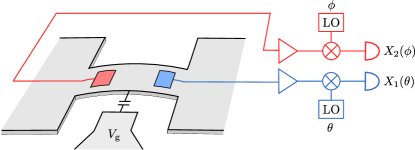
Figure 1: (Color online) Schematic illustration of a conceptual nanomechanical resonator with two homodyne measurement setups that probe two different modes of oscillation. The beam can oscillate in a large number of vibrational and flexural modes with different frequencies. The two homodyne detectors measure the mode quadratures $X_{1}(\phi)$ and $X_{2}(\theta)$ with frequencies $\omega_{1}/2\pi$ and $\omega_{2}/2\pi$, respectively. By analyzing the correlations between the $X_{1}(\phi)$ and $X_{2}(\theta)$ quadratures, it is possible to determine whether or not the mode states are quantum-mechanically entangled.

Here we consider the generation of nonclassical states and the subsequent violation of Bell inequalities by the use of similar intrinsic mechanical nonlinearitiesYamaguchi and Mahboob (2013); Lulla et al. (2012); Khan et al. (2013); Rips and Hartmann (2013). We focus on a model relevant to a recent experimental realization Mahboob et al. (2013) of a phonon laser, where a single mechanical device exhibits significant coupling between three internal modes of deformation, due to asymmetries in the beamYamaguchi and Mahboob (2013), and selective activation using external driving. Here we examine that same intrinsic inter-mode interaction in the quantum limit. A schematic illustration of the device considered here is shown in Fig. 1, though this is not intended to be representative of the ideal realization or measurement scheme for operating in the quantum limit. In most of our discussion we do not consider an explicit physical setup but rather focus on setting bounds on the fundamental system parameters necessary to realize the phenomena we discuss. The model we derive consists of an adiabatically-eliminated pump mode which drives the interaction between two lower-frequency signal and idler modes. We show that in the transient regime one can obtain violations of a Bell inequality based on correlations between quadrature measurements of the signal and idler modes. This is a re-imagining of a quintessential quantum optics experiment by using phonons that represent tangible mechanical vibrations.

This paper is organized as follows: In Sec. II we introduce the general model and the Hamiltonian for a nonlinear nanomechanical device. In Sec. II.1 we consider a regime in which a parametric oscillator is realized using three modes in the mechanical system, and in Sec. II.2 we introduce an effective two-mode model, valid when the pump mode can be adiabatically eliminated, and we analyze the types of nonclassical states that can be generated in this system. In Sec. III, we review Bell’s inequality using quadrature measurements, and in Sec. IV we analyze the conditions for realizing a violation of this quadrature-based Bell inequality with the mechanical system in the parametric oscillator regime studied in Sec. II.2. Finally we discuss the outlook for an experimental implementation using either intrinsic nonlinearities in Sec. V, or, as an alternative, optomechanical nonlinearities in Sec. V.1. We summarize our results in Sec. VII.

II Model

The general Hamiltonian for a nonlinear multimode resonator, describing both the self-nonlinearities and multimode couplings up to fourth-order, can be written as Khan et al. (2013)

$$H = \sum_{k}\omega_{k}a^{\dagger}_{k}a_{k}+\sum_{klm}\mathcal{\beta}_{klm}x_{k}x_{l}x_{m}$$ (1)

$$+ \sum_{klmn}\mathcal{\eta}_{klmn}x_{k}x_{l}x_{m}x_{n}+\mathcal{O}(x^{5}),$$

where $\omega_{k}$ is the frequency, $a_{k}$ is the annihilation operator, and $x_{k}=a_{k}+a_{k}^{\dagger}$ is the quadrature of the mechanical mode $k$. Here the basis has been chosen so that linear two-mode coupling terms are eliminated. The third-order mode-coupling tensor $\mathcal{\beta}_{klm}$ describes the odd-term self-nonlinearity and the trilinear multimode interaction. The fourth-order terms describes the even-term self-nonlinearity and fourth-order multimode coupling. In symmetric systems the fourth-order terms dominate (odd terms vanish due to symmetry), and it has been proposed elsewhere that they can be used to create effective mechanical qubitsRips and Hartmann (2013). The possible combination of both third and fourth-order terms will be briefly considered in the final section. The strength of the nonlinearity depends on the fundamental frequency (length) of the resonator, and can be enhanced by a range of techniquesRips and Hartmann (2013). In this work we focus on the three-mode coupling terms, as these are necessary to generate the states that violate continous variable Bell inequalities. Such terms vanish in symmetric systems and thus depend on the degree of asymmetry in the mechanical deviceKhan et al. (2013); Yamaguchi and Mahboob (2013), which again can be enhanced with fabrication techniques. Our approach in the following is to identify the ideal situation under which one can realize these rare Bell inequality violating states. Ultimately these states will be degraded by losses (which we investigate), but also by unwanted nonlinearities from the above hamiltonian.

II.1 Parametric oscillator regime

Figure 2: A visualization of the mode-matching condition required to obtain an effective three-mode system. The modes are represented as solid vertical lines, and the driving frequency and the sum of the signal and idler frequencies, which should sum up to a frequency close to $\omega_{0}$, are represented by dashed vertical lines.

Nanomechanical devices of the type described in the previous section have a large number of modes with different frequencies which depend on the microscopic structural properties of the beam. Here we focus on three such modes (relabelled as $k=0,1,2$) which are chosen such that they satisfy the phase-matching condition $\omega_{1}+\omega_{2}=\omega_{0}+\Delta_{0}$, where $\Delta_{0}\ll\omega_{0}$. In this case we can perform a rotating-wave approximation to single out the slowly-oscillating coupling terms, and obtain the desired effective three-mode system, neglecting any higher-order non-linearities. In the original frame, the Hamiltonian with this rotating-wave approximation is

$$H = \sum_{k=0}^{2}\omega_{k}a_{k}^{\dagger}a_{k}+i\kappa(a_{1}^{\dagger}a_{2}^{\dagger}a_{0}-a_{1}a_{2}a_{0}^{\dagger}),$$ (2)

where $a_{1}$ and $a_{2}$ are the signal and idler modes, respectively, and $a_{0}$ is the pump mode. Furthermore, we apply a driving force that is nearly resonant with $\omega_{0}$, with frequency $\omega_{L}=\omega_{0}-\Delta_{L}$, $|\Delta_{L}|\ll\omega_{0}$, and transform the above Hamiltonian to the rotating frame where the resonant drive terms are time-independent,

$$H = \Delta_{L}a_{0}^{\dagger}a_{0}+\sum_{k=1,2}\Delta_{k}a_{k}^{\dagger}a_{k}$$ (3)

$$+ i\kappa(a_{1}^{\dagger}a_{2}^{\dagger}a_{0}-a_{1}a_{2}a_{0}^{\dagger})-i(Ea_{0}^{\dagger}-E^{*}a_{0}).$$

Here $\Delta_{1}=\Delta_{2}=(\Delta_{0}-\Delta_{L})/2$, $\kappa=\beta_{012}$ is the inter-mode interaction strength, and $E$ is the driving amplitude of mode $a_{0}$. See Fig. 2 for a visual representation of the mode-matching condition and the detuning parameters $\Delta_{0}$ and $\Delta_{L}$.

This is an all-mechanical realization of the general three-mode parametric oscillator model in nonlinear optics Kheruntsyan and Petrosyan (2000); McNeil and Gardiner (1983), where mode $a_{0}$ is the quantized pump mode, and modes $a_{1}$ and $a_{2}$ are the signal and idler modes, respectively.

II.2 Effective two-mode model

We assume that in this purely nanomechanical realization of the parametric oscillator model, Eq. (3), all three mechanical modes interact with independent environments. We describe these processes with a standard Lindblad master equation on the form

$$\dot{\rho}=-i[H,\rho]+\sum_{k}\gamma_{k}\left\{(N_{k}+1)\mathcal{D}[a_{k}]+N_{k}\mathcal{D}[a_{k}^{\dagger}]\right\}\rho$$ (4)

where $\mathcal{D}[a_{k}]\rho=a_{k}\rho a_{k}^{\dagger}-\frac{1}{2}a_{k}^{\dagger}a_{k}\rho-\frac{1}{2}\rho a_{k}^{\dagger}a_{k}$ is the dissipator of mode $a_{k}$, $\gamma_{k}$ is the corresponding dissipation rate, and the average thermal occupation number is $N_{k}=\left(\exp(\hbar\omega_{k}\beta)-1\right)^{-1}$. Here $\beta=1/k_{B}T$ is the inverse temperature $T$, and $k_{B}$ is Boltzmann’s constant.

\begin{overpic}[width=216.81pt]{fig-3} \put(12.0,96.0){(a)} \put(54.0,96.0){(b)} \put(12.0,65.0){(c)} \end{overpic}

Figure 3: (Color online) Visualization of the steady state of the effective two-mode system. (a) The Fock state distribution of mode $a_{1}$ and $a_{2}$. (b) The single-mode Wigner function of mode $a_{1}$ and $a_{2}$. Both the Fock state distribution and the Wigner function are identical for both modes $a_{1}$ and $a_{2}$, due to the symmetric two-phonon processes and equal dissipation rates and initial states. The single-mode Wigner function is positive, and the single-mode state can therefore be considered classical. However, strong correlations exists between quadratures of two different modes, as shown in the joint quadrature probability distribution $P_{X_{1},X_{2}}(0,0)$ in (c). Here we have used the parameters $\kappa=0.15$, $E=0.094$, $\gamma_{0}=1.0$, $\gamma_{1}=\gamma_{2}=0$, and $\Delta_{0}=\Delta_{L}=0$. These parameters were chosen to produce a steady state that closely corresponds to the ideal stateMunro (1999) for quadrature Bell inequality violation, i.e. with $r=1.12$ (see Sec. IV.A).

Assuming that the pump mode is strongly damped compared to the signal and idler modes, $\gamma_{0}\gg\gamma_{1},\gamma_{2}$, and that the pump-mode dissipation dominates over the coherent interaction, $\gamma_{0}\gg\langle H\rangle\sim\kappa\langle a_{0}^{\dagger}a_{1}a_{2}\rangle$, one can adiabatically eliminateMcNeil and Gardiner (1983); Reid and Krippner (1993); Wiseman and Milburn (1993) the pump mode from the master equation given above. Here we also assume that the high-frequency pump mode is at zero temperature, $N_{0}=0$, while the temperatures of modes $a_{1}$ and $a_{2}$ can remain finite. This results in a two-mode master equation that includes correlated two-phonon dissipation, where one phonon from each mode dissipates to the environment through the pump mode, in addition to the original single-phonon losses in each mode:

$$\dot{\rho}= - i[H^{\prime},\rho]+\gamma\mathcal{D}[a_{1}a_{2}]\rho$$ (5)

$$+ \sum_{k=1,2}\gamma_{k}\left\{(N_{k}+1)\mathcal{D}[a_{k}]+N_{k}\mathcal{D}[a_{k}^{\dagger}]\right\}\rho,$$

where the effective two-phonon dissipation rate is

$$\gamma=\frac{\kappa^{2}\gamma_{0}/2}{|\gamma_{0}/2+i\Delta_{L}|^{2}}.$$ (6)

The reduced two-mode Hamiltonian is given by

$$H^{\prime} = \sum_{k=1,2}\Delta_{k}a_{k}^{\dagger}a_{k}+i(\mu a_{1}^{\dagger}a_{2}^{\dagger}-\mu^{*}a_{1}a_{2})+\chi a_{1}^{\dagger}a_{1}a_{2}^{\dagger}a_{2},$$

with the two-mode interaction strength

$$\mu=\frac{E\kappa}{\gamma_{0}/2+i\Delta_{L}},$$ (8)

and the effective cross-Kerr interaction strength

$$\chi=-\frac{\kappa^{2}\Delta_{L}}{|\gamma_{0}/2+i\Delta_{L}|^{2}},$$ (9)

which vanishes when the driving field is at exact resonance with the pump mode. In the following we will generally assume that this resonance condition can be reached, and $\Delta_{L}$ will be set to zero in the equations above.

In this resonant limit the Hamiltonian $H^{\prime}$ describes an ideal two-mode parametric amplifier, which is well-known to be the generator of two-mode squeezed states Reid and Drummond (1988). When applied to the vacuum state, or a low-temperature thermal state, the resulting two-modes squeezed states are nonclassically correlated Marian et al. (2003), but when viewed individually, both modes appear to be in thermal states. In spite of being quantum mechanically entangled, these two-mode squeezed states have a positive Wigner function and cannot violate the quadrature binning Bell inequalities Gilchrist et al. (1998) that we consider below. One must consider the effect of the two-phonon dissipation in Eq. [5] to induce such violations.

\begin{overpic}[width=216.81pt]{fig-4} \put(10.5,94.0){(a)} \put(10.5,71.0){(b)} \put(10.5,48.0){(c)} \put(10.5,25.0){(d)} \end{overpic}

Figure 4: (Color online) The time evolution of the phonon number (a), single-mode quadrature variances (b), and the variances of the two-mode quadrature differences (c), the logarithmic negativity (d), for the case when the state is initially in the zero-temperature ground state. In the large-time limit the state approaches the steady state that is visualized in Fig. 3. The single-mode variances increase above the vacuum limit as time increases, but the variance of cross-quadrature difference Var$(x_{1}-x_{2})$ decrease below the vacuum limit, which is a characteristic of two-mode squeezing, and the nonzero logarithmic negativity demonstrates that the steadystate is nonclassical. Here we used the same parameters as those given in the caption of Fig. 3.

In the highly idealized case when single phonon dissipation in the $a_{1}$ and $a_{2}$ modes is absent, i.e., $\gamma_{1}=\gamma_{2}=0$, but with $\gamma_{0}>0$, the model Eq. (5) produces a steady state Reid and Krippner (1993) of the form

$$\rho=\frac{1}{I_{0}(2r^{2})}\sum_{m,n}\frac{r^{2m+2n}}{m!n!}|m,m\rangle\langle n,n|,$$ (10)

where $I_{0}$ is the zeroth order modified Bessel function and $r=\sqrt{2E/\kappa}$. The special structure of this steady state, with equal number of phonons in each mode, is because both the Hamiltonian and two-phonon dissipator conserve the phonon-number difference $a_{2}^{\dagger}a_{2}-a_{1}^{\dagger}a_{1}$. However, this symmetry is broken if the single-phonon dissipation processes are included in the model, i.e. $\gamma_{1},\gamma_{2}>0$. The state Eq. (10) is visualized in Fig. 3, for the specific set of parameters given in the figure caption. Figure 3(a-b) show the Fock-state distribution and the Wigner function for the modes $a_{1}$ and $a_{2}$ (because of symmetry the states of both modes are identical in this case, and only one is shown). In this case the states of the two modes no longer appear to be thermal when viewed individually, but the reduced single-mode Wigner functions are positive and thus, on their own, each mode appears classical. However, together, the two-mode Wigner function can be negative. For example, there is a strong cross-quadrature correlation, as shown in Fig. 3(c). The variances of the cross-quadrature differences, in the transient approach to the steady state, are shown in Fig. 4, and exactly in the steady state the variance of the squeezed two-mode operator difference is

$${\rm Var}(x_{1}-x_{2})=1+2r^{2}\frac{I_{1}(2r^{2})}{I_{0}(2r^{2})}-2r^{2},$$ (11)

which in the limit of large $r$ approaches 1/2, but has a local minimum of about 0.4 at $r\approx 0.92$. We note that for the vacuum state ${\rm Var}(x_{1}-x_{2})=1$, and thus this quadrature difference variance is therefore squeezed below the vacuum level for any $r>0$. The logarithmic negativity Adesso and Illuminati (2007) shown in Fig. 4(d) further demonstrates the nonclassical nature of this state.

These intermode quadrature correlations, with squeezing below the vacuum level of fluctuations, are nonclassical and it has been shown that this particular state can violate Bell inequalities based on quadrature measurements Gilchrist et al. (1998), as we will discuss in the next section. In fact, this steady state is, for a certain value of $r$, a good approximation to the ideal two-mode quantum state Munro (1999) for these kind of Bell inequalities. However, it has also been shown that in the presence of single phonon dissipation the steady state two-mode Wigner function is always positive, and thus exhibits a hidden-variables description and cannot violate any Bell inequalities Kheruntsyan and Petrosyan (2000). Fortunately, this is only the case for the steady state, and there can be a significant transient period in which the two-mode system is in a state that can give a violation.

In the following we consider two regimes; the steady state, and the slow transient dynamics of a system that is originally in the ground state, and approaches the new steady state after the driving field has been turned on.

III Bell inequalities for nanomechanical systems

Verifying that a nanomechanical system is in the quantum regime, and that the states produced in the system are nonclassical, can be sometimes be experimentally challenging, largely because of the difficulty in implementing single-phonon detectors in nanomechanical systems. As has been done in circuit QED Fink et al. (2008); Schuster et al. (2008), measuring a nonlinear energy spectrum Rips and Hartmann (2013) would be a convincing indication that the system is operating in the quantum regime, although it does not imply that the state of the system is nonclassical, and all quantum nanomechanical systems need not necessarily be nonlinear. A number of techniques could be used to demonstrate that the state is nonclassical Miranowicz et al. (2010), for example reconstructing the Wigner function using state tomography and looking for negative values, or evaluating entanglement measures such as the logarithmic negativity (for Gaussian states) or entanglement entropy (suitable only at zero temperature).

Here we are interested in a nonclassicality test that can be evaluated using joint two-mode quadrature measurements. The two-mode squeezing shown in the previous section can be considered as an entanglement witnessSimon (2000); Duan et al. (2000), and was recently investigated experimentally in an opto-mechanical devicePalomaki et al. (2013a, b). The quadrature-based Bell inequality can be seen as another, stricter, example of a nonclassicality test, and in the following we focus on the possibility of violating these Bell inequalities with the nanomechanical system outlined in the previous section. Even though one cannot rule out the locality-loophole in such a system, and thus a violation would lack any meaning as a strict test of Bell nonlocality Brunner et al. (2013), it would still serve as a very satisfying test for two-mode entanglement.

The original Bell inequalities are formulated for dichotomic measurements, with two possible outcomes. However, dichotomic measurements are not normally available in harmonic systems like the nanomechanical systems considered here, where the measurement outcomes are, for the most part, continuous and unbound. In this continuous-variable limit one must choose how to perform a Bell inequality test with care. Generalized inequalities for unbound measurements existCavalcanti et al. (2007), but are both extremely challenging to implement and hard to violate. Fortunately one can implement CHSH-type Bell inequality by binning quadrature measurements, and thus obtaining a dichotomic bound observable. Munro Munro (1999) showed that, while in general it is hard to generate states which can violate such an inequality, it is possible to generate precisely the type of states which do cause a violation with a nondegenerate parametric oscillator, which is analogous to the system we investigate here.

One possible binning strategyGilchrist et al. (1998); Wenger et al. (2003) for the continuous outcomes of quadrature measurements of the mechanical modes is to classify the outcomes as $1$ if the measurement outcome is $X_{\theta}>0$, and $0$ otherwise. The probability of the outcomes $0$ and $1$ for the two modes can then be written

$$P_{\alpha\beta}(\theta,\phi) = \int_{L(\alpha)}^{U(\alpha)}\int_{L(\beta)}^{U(\beta)}d^{2}Xp(X_{1}^{\theta},X_{2}^{\phi})[\rho]$$ (12)

where

$$L(\alpha)=\begin{cases}0&\text{if $\alpha=1$}\\ -\infty&\text{if $\alpha=0$}\end{cases},U(\alpha)=\begin{cases}\infty&\text{if $\alpha=1$}\\ 0&\text{if $\alpha=0$}\end{cases}.$$ (13)

Here $\rho$ is the two-mode density matrix and $p(X_{1}^{\theta},X_{2}^{\phi})[\rho]$ is the probability distribution for obtaining the measurement outcomes $X_{1}^{\theta}$ and $X_{2}^{\phi}$ for the signal and idler mode quadratures

$$x_{1}^{\theta} = a_{1}e^{-i\theta}+a_{1}^{\dagger}e^{i\theta},$$ (14)

$$x_{2}^{\phi} = a_{2}e^{-i\phi}+a_{2}^{\dagger}e^{i\phi},$$ (15)

respectively. This probability distribution is given by

$$p(X_{1}^{\theta},X_{2}^{\phi})[\rho]=\left<X_{1}^{\theta},X_{2}^{\phi}\right|\rho\left|X_{1}^{\theta},X_{2}^{\phi}\right>$$

$$= \sum_{m,n,p,q}\rho_{(m,n),(p,q)}\frac{e^{-i(m\theta+n\phi)}e^{i(p\theta+q\phi)}}{\pi\sqrt{2^{m+n+p+q}m!n!p!q!}}$$

$$\times e^{-X_{1}^{2}}e^{-X_{2}^{2}}H_{m}(X_{1})H_{n}(X_{2})H_{p}(X_{1})H_{q}(X_{2})$$

where $H_{n}(x)$ is the Hermite polynomial of $n$th order, and where we have written the density matrix in the two-mode Fock basis,

$$\rho=\sum_{m,n,p,q}\rho_{(m,n),(p,q)}\left|m,n\rangle\langle p,q\right|.$$ (17)

The integral in Eq. (12) can be evaluated analyticallyMunro (1999), but in general the sum in Eq. (III) cannot.

Treating the binned quadrature measurements as dichotomic observables we can write the standard Bell’s inequalities in the Clauser-Horne (CH) Clauser and Horne (1974) form

$$B_{\rm CH}=\frac{P_{11}(\theta,\phi)-P_{11}(\theta,\phi^{\prime})+P_{11}(\theta^{\prime},\phi)+P_{11}(\theta^{\prime},\phi^{\prime})}{P_{1}(\theta^{\prime})+P_{1}(\phi)}$$ (18)

which for a classical state satisfies $|B_{\rm CH}|\leq 1$, and in the Clauser-Horne-Shimony-Holt (CHSH) Clauser et al. (1969) form

$$B_{\rm CHSH} = E(\theta,\phi)-E(\theta^{\prime},\phi)+E(\theta,\phi^{\prime})+E(\theta^{\prime},\phi^{\prime}),\;\;$$ (19)

$$E(\theta,\phi) = P_{11}(\theta,\phi)+P_{00}(\theta,\phi)$$ (20)

$$- P_{10}(\theta,\phi)-P_{01}(\theta,\phi),$$

which for a classical state satisfies $|B_{\rm CHSH}|\leq 2$. Here we have also used

$$P_{1}(\theta) = \int_{0}^{\infty}\int_{-\infty}^{\infty}d^{2}Xp(X_{1}^{\theta},X_{2}^{\phi})[\rho].$$ (21)

Both $B_{\rm CH}$ and $B_{\rm CHSH}$ are in general functions of the four angles $\theta,\phi,\theta^{\prime}$, and $\phi^{\prime}$. However, to reduce the number of parameters here we consider the angle parameterization $\theta=-2\varphi$, $\phi=3\varphi$, $\theta^{\prime}=0$, and $\phi^{\prime}=\varphi$, which only leaves a single free angle parameter $\varphi$. In principle this can reduce the magnitude of violation one can observe, but as we will see this parameterization still allows violations to occur for the types of states we are interested in here. In the following we evaluate both $B_{\rm CH}$ and $B_{\rm CHSH}$ using this angle parameterization.

IV Violation of Bell’s inequality with nanomechanical resonators

In this section we investigate the conditions under which the states formed in the multimode nanomechanical system may violate Bell’s inequality. We emphasize again that in this context we are interested in Bell’s inequality as a test that can demonstrate entanglement between different mechanical modes. We begin with an analysis of the steadystate for the idealized model with $\gamma_{1},\gamma_{2}=0$, and then turn our attention to the transient behaviour for finite $\gamma_{1}$ and $\gamma_{2}$.

IV.1 Steady state

With $\gamma_{1},\gamma_{2}=0$, the steady state is given by Eq. (10), and inserting this state in the Bell inequalities Eqs. (18-19) gives an expression as a function of the steady state parameter $r$ and the angle $\varphi$ that can be optimized for maximum Bell violation. The optimal value of the angle turns out to be $\varphi=\pi/4$, and the resulting equation for optimal $r$ is

$$I_{0}(2r^{2})\frac{dG(r)}{dr}=4r^{2}I_{1}(2r^{2})G(r),$$ (22)

but the sum over Fock-state basis that comes from Eq. (III) cannot to our knowledge be evaluated in a simple analytical form, so we have

$$G(r) = \sum_{n}\sum_{m>n}\frac{8(2r^{2})^{n+m}\pi}{(n!m!)^{2}(n-m)^{2}}\left[\mathcal{F}(n,m)-\mathcal{F}(m,n)\right]^{2}\times$$ (23)

$$\left\{3\cos\left[(n-m)\varphi\right]-\cos\left[3\varphi(n-m)\right]\right\},$$

and

$$\mathcal{F}(n,m)=\left[\Gamma\left(\frac{1}{2}-\frac{n}{2}\right)\Gamma\left(-\frac{m}{2}\right)\right]^{-1},$$ (24)

as given in Ref. Munro, 1999. Solving Eq. (22) numerically gives $r_{\rm opt}\approx 1.12$, as reported in Ref. Gilchrist et al., 1998. The corresponding steady state Eq. (10) for $r_{\rm opt}$ is visualized in Fig. 3. We note that for this optimal Bell violating state the mean phonon number in each mode is only $\langle n\rangle\approx 0.94$, which highlights the need to operate the system near its ground state. If fact, when $\langle n\rangle\gg 1$ no Bell inequality violation can be observed.

In our nanomechnical model this translates to an optimal driving strength, $E_{\rm opt}=r_{\rm opt}^{2}\kappa/2$, that maximizes the Bell inequality violation for a given nonlinearity $\kappa$. This optimal driving amplitude $E_{\rm opt}$ applies to the steady state of the idealized model without single-phonon dissipation. With finite single-phonon dissipation, the steady state does not violate any of the Bell inequalities. However, as we will see in the following section, $E_{\rm opt}$ still gives a good approximation for the optimal transient violation. While these transients are harder to capture, recent experiments on opto-mechanical systems have shown they are in principle possible Palomaki et al. (2013a, b), and relevant for the alternative proposal in the final section below. How far one can go with using multiple ancilla optical or microwave cavities to perform similar measurements on different internal modes of a single mechanical device is not yet clear.

IV.2 Transient

\begin{overpic}[width=216.81pt]{fig-5-a}\put(10.0,62.0){(a)}\end{overpic}

\begin{overpic}[width=216.81pt]{fig-5-b}\put(10.0,64.0){(b)}\end{overpic}

Figure 5: (Color online) (a) The normalized CH and CHSH Bell quantities (violation above 1) as a function of time, for the pumped two-mode nanomechanical resonator, under the ideal condition without signal and idler mode dissipation (dashed) and for the case including signal and idler dissipation. The initial state is the vacuum state, which we assume can be prepared to a good approximation using cooling. At $t=0$, the parametric amplification is turned on by the activation of the driving field with amplitude $E$. In the ideal case, the steady state violates both the CH and CHSH Bell inequalities, but there is no steady state violation when single-phonon dissipation is included. However, there is a period of time during the transient where both inequalities are violated. (b) The angle $\varphi$ dependence for the normalized CH and CHSH Bell quantities for $t\gamma_{0}/\kappa^{2}=1.8$, where solid lines include dissipation and dashed lines are the ideal case. The optimal value of $\varphi$ for the states produced in the model we investigate here is $\varphi=\pi/4$, which was used in (a). The parameters used here are the same as in Fig. 3, and for the solid lines we used $\gamma_{1}=\gamma_{2}=0.001$.

\begin{overpic}[width=138.75826pt]{fig-6-a} \put(-3.0,60.0){(a)}\end{overpic}

\begin{overpic}[width=138.75826pt]{fig-6-b} \put(-3.0,60.0){(b)}\end{overpic}

\begin{overpic}[width=138.75826pt]{fig-6-c} \put(-3.0,60.0){(c)}\end{overpic}

\begin{overpic}[width=138.75826pt]{fig-6-d} \put(-3.0,60.0){(d)}\end{overpic}

\begin{overpic}[width=138.75826pt]{fig-6-e} \put(-3.0,60.0){(e)}\end{overpic}

\begin{overpic}[width=138.75826pt]{fig-6-f} \put(-3.0,60.0){(f)}\end{overpic}

Figure 6: (Color online) Violation of the normalized quadrature CHSH Bell inequality (redish region) as a function of time $t$ and the inter-mode coupling $\kappa$ (a,d), the pump mode driving amplitude $E$ (b,e), and the pump-mode dissipation rate $\gamma_{0}$ (c,f). The ideal case without signal and idler mode dissipation is shown in (a-c), and (d-e) include signal and idler mode dissipation with equal dissipation rates $\gamma_{1}=\gamma_{2}=0.001$. In (a-c) there is a parameter window for $\kappa$ and $E$ which results in a violation for sufficiently large $t$, as well as in the steady state. However, in (d-e) there is no violation in the steady state, but during a transient time a violation may still occur for suitably chosen parameters. Apart from the parameters on the vertical axes, the parameters were kept fixed at the same values as given in Fig. 3, and denoted by a bar over the symbol in the axes.

Since the more realistic model, with finite single-phonon dissipation processes, does not produce a steady state that violates any of the Bell inequalities, we are lead to investigate transient dynamics. Here we focus on the transient which occurs when the driving field $E$ is turned on after the relevant modes have been cooled to their ground states. The state of the system then evolves from the ground state to the steady state that does not violate the Bell inequalities. However, if the single phonon dissipation processes are sufficiently slow there can be a significant time interval during which the state of the system does violate the Bell inequalities.

To investigate this transient dynamics we numerically evolve the effective two-mode system described by the master equation, Eq. (5), and evaluate the $B_{\rm CH}$ and $B_{\rm CHSH}$ quantities as a function of time and the angle $\varphi$. The results shown in Fig. 5, for the situations with and without signal and idler mode dissipation and at zero temperature, demonstrate that the nanomechanical system we consider can indeed be driven into a transient state that violates both types of Bell inequalities. With losses the onset of violation is proportional to $\gamma_{0}/\kappa^{2}$, and the time at which the violation cease is proportional to $\gamma_{1}^{-1},\gamma_{2}^{-1}$, so if

$$\gamma_{1},\gamma_{2}\ll\kappa^{2}/\gamma_{0},$$ (25)

we expect a significant period of time during the transient where the inequalities will be violated. We note that in Fig. 5(a), the regions of violation for the CH and CHSH inequalities are identical, and this is, according to our observations, always the case for this model and angle parametrization. Because of this, in the following we only show the results for the CHSH inequality.

To further explore the parameter space that can produce a Bell-inequality violation we evolve the master equation as a function of time and the parameters $E$, $\kappa$ and $\gamma_{0}$, for both the ideal case with dissipation-less signal and idler modes, $\gamma_{1}=\gamma_{2}=0$, and for the case including signal and idler mode dissipation, $\gamma_{1},\gamma_{2}>0$. In these simulations the initial state is always the ground state, and we take the temperature of the signal and idler modes to be zero. The results are shown in Fig. 6(a-c) and (e-f), respectively. From Fig. 6 it is clear that for the case $\gamma_{1}=\gamma_{2}=0$, there exist optimal values of $\kappa$ and $E$, given that other parameters are fixed, that produce steady states that maximally violates the Bell inequality (marked with dashed lines in the figures). However, importantly, we also note that the optimal values for $\kappa$ and $E$ for the steady state of the ideal model also give a good indicator for the optimal regime for the Bell violation in the transient of the case with finite single-phonon dissipation, when additionally taking into account the time scales for the transient given in Eq. (25).

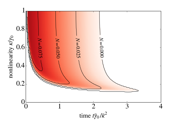
Figure 7: (Color online) The regions where a transient Bell inequality violation can be achieved, as a function of nonlinearity $\kappa$ and time $t$, and for different temperatures. The region of violation at zero temperature is shown in redish color. The contours mark the regions of violation for finite signal and idler mode temperatures (assumed equal), labeled by the average number $N$ of thermal phonons. We note that even a very small number of initial thermal phonons inhibits the Bell inequality violation, which suggest that excellent ground-state cooling of both modes is a prerequisite to obtaining a violation.

When the signal and idler modes have finite temperature the region of Bell inequality violation is further reduced, as shown in Fig. 7. The detrimental effects of thermal phonons are two-fold: It reduces the transient time-interval during which a violation can be observed, and the nonlinear interaction strength required to be able to see any violation at all increases. In fact, to observe a transient Bell inequality violation, the average thermal occupation number must be very small: An average thermal occupation number of even $0.1$ phonon in the signal and idler mode is sufficient to inhibit any Bell violation with the system we have considered here. Excellent ground state cooling is therefore a prerequisite to violating a Bell inequality tests in a nanomechanical resonator.

V Experimental outlook

As can be seen in Fig. 6 and Fig. 7, the violation of a Bell inequality in the system we consider here requires, as expected, a combination of low temperature, large nonlinearity, and transient quadrature measurements. These conditions can all be rather challenging to satisfy in an experimental system, but on the other hand they are exactly the type of conditions that one can expect would have to be satisfied for realistic quantum mechanical applications in these devices. The Bell inequality violation can therefore be seen as a benchmark that indicates that entangled quantum states can be generated and detected with high precision.

While one can imagine cryogenics and side-band cooling techniques can satisfy the first criteria O’Connell et al. (2010); Teufel et al. (2011); Chan et al. (2011); Grajcar et al. (2008), the ultimate upper limit of the strength of intrinsic nonlinearities in mechanical systems is not clear. In a recent experiment extremely large nonlinear intra-mode coupling was observed in a carbon nanotube system when the modes had frequencies which were integer multiples of each other Sapmaz et al. (2003). In that case a strong effective mode-mode coupling was also found, which is required for generating the Bell inequality violating states we consider here. Nonlinear mode coupling has also been demonstrated and analyzed in doubly-clamped beam resonators Westra et al. (2010); Lulla et al. (2012); Khan et al. (2013); Yamaguchi and Mahboob (2013), and circular graphene membrane resonators Eriksson et al. (2013). Also, recent studiesRips and Hartmann (2013) have proposed enhancing the nonlinearity per phonon by reducing the fundamental frequency of the mechanical oscillator, which essentially amounts to increasing the ground state displacement. Thus, there is progress in realizing nonlinear mode interaction in several types of nanomechanical systems, and sufficiently strong nonlinearities to produce Bell inequality violating states should be obtainable in these devices, although further progress in this experimental work in this direction may be required.

Performing transient quadrature measurements of selected modes of the mechanical resonator is an another experimental challenge. However, the displacement of a nanomechanical resonator can be converted to electrical signals and measured for example using a range of different techniques, for example piezoelectric schemes Mahboob et al. (2012), coupling to auxiliary optical modes Bochmann et al. (2013); Paternostro et al. (2007), or by capacitive coupling to a microwave circuit Regal et al. (2008). In recent experiments, transient quadrature measurements of a nanomechanical system were carried out with high precision and level of control Palomaki et al. (2013a, b). Aslo, in microwave electronics, quadrature measurements in the quantum regime have been applied to measure two-mode squeezing Eichler et al. (2011b); Bergeal et al. (2012), state tomography Mallet et al. (2011), and entanglement Flurin et al. (2012). Given a sufficiently efficient transducer from mechanical displacement to electrical signals, the outlook for the required measurements for evaluating the quadrature Bell inequality is therefore encouraging.

V.1 Optomechanical realization

As an alternative to the purely mechanical scheme discussed so far one could observe the similar quadrature-based Bell inequality violations in an optomechanical setup akin to that proposed in Refs. Stannigel et al., 2011 and Ludwig et al., 2012, where a single mechanical mode is coupled to two optical cavities, e.g., in a membrane-in-the-middle geometry or within a photonic crystal cavity. The most straightforward implementation would be to use the mechanical mode as the pump mode which then acts to entangle the optical modes. The optical modes are coupled due to a photon tunneling, and the resulting hybridized modes replace the mechanical signal and idler modes $a_{1}$ and $a_{2}$ we discussed in this work. On resonance this again leads to the same interaction we use in Eq. [2]. The main motivation of inducing this interaction in these earlier works was to engineer anharmonic energy levels. This anharmonicity allows specific transitions to be addressed with external laser fields allowing one to use such devices as single-phonon/photon transistors and for non-demolition measurements of phonons or photons. In the limit where the mechanical pump mode can be driven and adiabatically eliminated, one in principle observe Bell inequality violations in the (hybridized) quadrature measurements of the two optical cavities.

VI Combining even and odd nonlinearities: coupling mechanical qubits

In the previous calculations we have been exclusively considering the effect of odd nonlinearities which can only arise in asymmetric mechanical systems. In purely symmetric devices the even order terms dominate, arguably the most important of which is the $x^{4}$ Duffing nonlinearity. Recent works Rips and Hartmann (2013) have examined how this induces an anharmonic energy spectrum in the fundamental mode of a nanomechanical system, and outlined how this anharmonic spectrum can be used as an effective qubit for quantum computation. Naturally one can consider the effect of both the third order coupling we have outlined here, and the third and fourth order Duffing self-anharmonicity. Ultimately the relative strengths of these different terms depend strongly on the overlap between the different mode shapes within the device, the geometry of the device, and the effect of various nonlinearity enhancing mechanisms. A naive investigation of the contributions from these quartic terms suggest they only work to degrade the Bell inequality violation we discuss here. However, going beyond the regime we have outlined thus far, one may note that, by changing the frequency of the driving field in Eq. (1) one can get an excitation-preserving beam-splitter type of interaction between the signal and idler modes.

$$H_{\rm int}^{c}=\mu(a_{1}^{\dagger}a_{2}+a_{2}^{\dagger}a_{1}).$$ (26)

If this is combined with a sufficiently strong third or fourth-order self nonlinearity, such that the lowest lying energy states of each mode can be considered as a two-level system, one has a means to couple different mechanical qubits in a single device. It may be possible to construct similar interactions with ancilla cavities and optomechanical interactions Stannigel et al. (2011); Jacobs (2012). The original parametric interaction described in Eq. (3) is not useful for this purpose as it takes one out of a single excitation subspace, as does the two-phonon dissipation.

VII Conclusions

We have investigated a regime of a multimode nanomechanical resonator, with intrinsic nonlinear mode coupling, in which three selected modes realize a parametric oscillator. In the regime where the pump mode of the parametric oscillator can be adiabatically eliminated, we have investigated the generation of entangled states between two distinct modes of oscillation in the nanomechanical resonator, and the possibility of detecting this entanglement using quadrature-based Bell inequality tests. Our results demonstrate that while realistically it will not be possible to violate any Bell inequality in the steady state, there can be a significant duration of time in which the transient evolution from the ground state (prepared by cooling) to the steady state where the state of the system violates Bell inequalities. However, to achieve this transient violation requires a relatively large nonlinear mode coupling, excellent ground state cooling, and fast and efficient quadrature measurements. These are, of course, very challenging experimental requirements, but we believe that if a quadrature Bell inequality violation is realized experimentally it would be a very strong demonstration of quantum entanglement in a macroscopic mechanical system.

References

- Cleland (2002) A. Cleland, Foundations of Nanomechanics, Advanced Texts in Physics (Springer, 2002).
- Blencowe (2004) M. Blencowe, Physics Reports 395, 159 (2004).
- Poot and van der Zant (2012) M. Poot and H. S. van der Zant, Physics Reports 511, 273 (2012).
- Aspelmeyer et al. (2013) M. Aspelmeyer, T. J. Kippenberg, and F. Marquardt, arXiv:1303.0733 (2013).
- O’Connell et al. (2010) A. D. O’Connell, M. Hofheinz, M. Ansmann, R. C. Bialczak, M. Lenander, E. Lucero, M. Neeley, D. Sank, H. Wang, M. Weides, et al., Nature 464, 697 (2010).
- Teufel et al. (2011) J. D. Teufel, T. Donner, D. Li, J. W. Harlow, M. S. Allman, K. Cicak, A. J. Sirois, J. D. Whittaker, K. W. Lehnert, and R. W. Simmonds, Nature 475, 359 (2011).
- Chan et al. (2011) J. Chan, T. P. M. Alegre, A. H. Safavi-Naeini, J. T. Hill, A. Krause, S. Groblacher, M. Aspelmeyer, and O. Painter, Nature 478, 89 (2011).
- Regal et al. (2008) C. A. Regal, J. D. Teufel, and K. W. Lehnert, Nat Phys 4, 555 (2008).
- Sun et al. (2006) C. P. Sun, L. F. Wei, Y.-x. Liu, and F. Nori, Phys. Rev. A 73, 022318 (2006).
- Wallquist et al. (2009) M. Wallquist, K. Hammerer, P. Rabl, M. Lukin, and P. Zoller, Physica Scripta 2009, 014001 (2009).
- Safavi-Naeini and Painter (2011) A. H. Safavi-Naeini and O. Painter, New Journal of Physics 13, 013017 (2011).
- Xiang et al. (2013) Z.-L. Xiang, S. Ashhab, J. Q. You, and F. Nori, Rev. Mod. Phys. 85, 623 (2013).
- Bochmann et al. (2013) J. Bochmann, A. Vainsencher, D. D. Awschalom, and A. N. Cleland, Nat Phys 9, 712 (2013).
- Rips and Hartmann (2013) S. Rips and M. J. Hartmann, Phys. Rev. Lett. 110, 120503 (2013).
- Tian et al. (2008) L. Tian, M. S. Allman, and R. W. Simmonds, New Journal of Physics 10, 115001 (2008).
- Jähne et al. (2009) K. Jähne, C. Genes, K. Hammerer, M. Wallquist, E. S. Polzik, and P. Zoller, Phys. Rev. A 79, 063819 (2009).
- Stannigel et al. (2011) K. Stannigel, P. Rabl, A. S. Sørensen, M. D. Lukin, and P. Zoller, Phys. Rev. A 84, 042341 (2011).
- Wang and Clerk (2013) Y.-D. Wang and A. A. Clerk, Phys. Rev. Lett. 110, 253601 (2013).
- Westra et al. (2010) H. J. R. Westra, M. Poot, H. S. J. van der Zant, and W. J. Venstra, Phys. Rev. Lett. 105, 117205 (2010).
- Lulla et al. (2012) K. J. Lulla, R. B. Cousins, A. Venkatesan, M. J. Patton, A. D. Armour, C. J. Mellor, and J. R. Owers-Bradley, New Journal of Physics 14, 113040 (2012).
- Khan et al. (2013) R. Khan, F. Massel, and T. T. Heikkilä, Phys. Rev. B 87, 235406 (2013).
- Yamaguchi and Mahboob (2013) H. Yamaguchi and I. Mahboob, New Journal of Physics 15, 015023 (2013).
- Clerk et al. (2008) A. A. Clerk, F. Marquardt, and K. Jacobs, New Journal of Physics 10, 095010 (2008).
- Liao and Law (2011) J.-Q. Liao and C. K. Law, Phys. Rev. A 83, 033820 (2011).
- Palomaki et al. (2013a) T. A. Palomaki, J. W. Harlow, J. D. Teufel, R. W. Simmonds, and K. W. Lehnert, Nature 495, 210 (2013a).
- Palomaki et al. (2013b) T. A. Palomaki, J. D. Teufel, R. W. Simmonds, and K. W. Lehnert, Science 8, 710 (2013b).
- Lemonde et al. (2013) M.-A. Lemonde, N. Didier, and A. A. Clerk, Phys. Rev. Lett. 111, 053602 (2013).
- Qian et al. (2012) J. Qian, A. A. Clerk, K. Hammerer, and F. Marquardt, Phys. Rev. Lett. 109, 253601 (2012).
- Nation (2013) P. D. Nation, Phys. Rev. A 88, 053828 (2013).
- Lörch et al. (2013) N. Lörch, J. Qian, A. Clerk, F. Marquardt, and K. Hammerer, arXiv:1310.1298 (2013).
- Rips et al. (2012) S. Rips, M. Kiffner, I. Wilson-Rae, and M. J. Hartmann, New Journal of Physics 14, 023042 (2012).
- Tian (2005) L. Tian, Phys. Rev. B 72, 195411 (2005).
- Voje et al. (2012) A. Voje, J. M. Kinaret, and A. Isacsson, Phys. Rev. B 85, 205415 (2012).
- Xue et al. (2007) F. Xue, Y.-x. Liu, C. P. Sun, and F. Nori, Phys. Rev. B 76, 064305 (2007).
- Cohen and Di Ventra (2013) G. Z. Cohen and M. Di Ventra, Phys. Rev. B 87, 014513 (2013).
- Tan et al. (2013) H. Tan, G. Li, and P. Meystre, Phys. Rev. A 87, 033829 (2013).
- Xu et al. (2013) X.-W. Xu, Y.-J. Zhao, and Y.-x. Liu, Phys. Rev. A 88, 022325 (2013).
- Suh et al. (2010) J. Suh, M. D. LaHaye, P. M. Echternach, K. C. Schwab, and M. L. Roukes, Nano Letters 10, 3990 (2010).
- Massel et al. (2011) F. Massel, T. T. Heikkila, J.-M. Pirkkalainen, S. U. Cho, H. Saloniemi, P. J. Hakonen, and M. A. Sillanpaa, Nature 480, 351 (2011).
- Eichler et al. (2011a) A. Eichler, J. Moser, J. Chaste, M. Zdrojek, I. Wilson-Rae, and A. Bachtold, Nat. Nano. 6, 339 (2011a).
- Voje et al. (2013) A. Voje, A. Isacsson, and A. Croy, Phys. Rev. A 88, 022309 (2013).
- Jacobs (2012) K. Jacobs, arXiv:1209.2499 (2012).
- Mahboob et al. (2013) I. Mahboob, K. Nishiguchi, A. Fujiwara, and H. Yamaguchi, Phys. Rev. Lett. 110, 127202 (2013).
- Kheruntsyan and Petrosyan (2000) K. V. Kheruntsyan and K. G. Petrosyan, Phys. Rev. A 62, 015801 (2000).
- McNeil and Gardiner (1983) K. J. McNeil and C. W. Gardiner, Phys. Rev. 28, 1560 (1983).
- Munro (1999) W. J. Munro, Phys. Rev. A 59, 4197 (1999).
- Reid and Krippner (1993) M. D. Reid and L. Krippner, Phys. Rev. A 47, 552 (1993).
- Wiseman and Milburn (1993) H. M. Wiseman and G. J. Milburn, Phys. Rev. A 47, 642 (1993).
- Reid and Drummond (1988) M. D. Reid and P. D. Drummond, Phys. Rev. Lett. 60, 2731 (1988).
- Marian et al. (2003) P. Marian, T. A. Marian, and H. Scutaru, Phys. Rev. A 68, 062309 (2003).
- Gilchrist et al. (1998) A. Gilchrist, P. Deuar, and M. D. Reid, Phys. Rev. Lett. 80, 3169 (1998).
- Adesso and Illuminati (2007) G. Adesso and F. Illuminati, Journal of Physics A: Mathematical and Theoretical 40, 7821 (2007).
- Fink et al. (2008) J. M. Fink, M. Göppl, M. Baur, R. Bianchetti, P. J. Leek, A. Blais, and A. Wallraff, Nature 454, 315 (2008).
- Schuster et al. (2008) I. Schuster, A. Kubanek, A. Fuhrmanek, T. Puppe, P. W. H. Pinkse, K. Murr, and G. Rempe, Nature Physics 4, 382 (2008).
- Miranowicz et al. (2010) A. Miranowicz, M. Bartkowiak, X. Wang, Y.-x. Liu, and F. Nori, Phys. Rev. A 82, 013824 (2010).
- Simon (2000) R. Simon, Phys. Rev. Lett. 84, 2726 (2000).
- Duan et al. (2000) L.-M. Duan, G. Giedke, J. I. Cirac, and P. Zoller, Phys. Rev. Lett. 84, 2722 (2000).
- Brunner et al. (2013) N. Brunner, D. Cavalcanti, S. Pironio, V. Scarani, and S. Wehner, arXiv:1303.2849 (2013).
- Cavalcanti et al. (2007) E. G. Cavalcanti, C. J. Foster, M. D. Reid, and P. D. Drummond, Phys. Rev. Lett. 99, 210405 (2007).
- Wenger et al. (2003) J. Wenger, M. Hafezi, F. Grosshans, R. Tualle-Brouri, and P. Grangier, Phys. Rev. A 67, 012105 (2003).
- Clauser and Horne (1974) J. F. Clauser and M. A. Horne, Phys. Rev. D 10, 526 (1974).
- Clauser et al. (1969) J. F. Clauser, M. A. Horne, A. Shimony, and R. A. Holt, Phys. Rev. Lett. 23, 880 (1969).
- Grajcar et al. (2008) M. Grajcar, S. Ashhab, J. R. Johansson, and F. Nori, Phys. Rev. B 78, 035406 (2008).
- Sapmaz et al. (2003) S. Sapmaz, Y. M. Blanter, L. Gurevich, and H. S. J. van der Zant, Phys. Rev. B 67, 235414 (2003).
- Eriksson et al. (2013) A. M. Eriksson, D. Midtvedt, A. Croy, and A. Isacsson, Nanotechnology 24, 395702 (2013).
- Mahboob et al. (2012) I. Mahboob, K. Nishiguchi, H. Okamoto, and H. Yamaguchi, Nat Phys 8, 387 (2012).
- Paternostro et al. (2007) M. Paternostro, D. Vitali, S. Gigan, M. S. Kim, C. Brukner, J. Eisert, and M. Aspelmeyer, Phys. Rev. Lett. 99, 250401 (2007).
- Eichler et al. (2011b) C. Eichler, D. Bozyigit, C. Lang, M. Baur, L. Steffen, J. M. Fink, S. Filipp, and A. Wallraff, Phys. Rev. Lett. 107, 113601 (2011b).
- Bergeal et al. (2012) N. Bergeal, F. Schackert, L. Frunzio, and M. H. Devoret, Phys. Rev. Lett. 108, 123902 (2012).
- Mallet et al. (2011) F. Mallet, M. A. Castellanos-Beltran, H. S. Ku, S. Glancy, E. Knill, K. D. Irwin, G. C. Hilton, L. R. Vale, and K. W. Lehnert, Phys. Rev. Lett. 106, 220502 (2011).
- Flurin et al. (2012) E. Flurin, N. Roch, F. Mallet, M. H. Devoret, and B. Huard, Phys. Rev. Lett. 109, 183901 (2012).
- Ludwig et al. (2012) M. Ludwig, A. H. Safavi-Naeini, O. Painter, and F. Marquardt, Phys. Rev. Lett 109, 063601 (2012).
- Johansson et al. (2012) J. R. Johansson, P. D. Nation, and F. Nori, Comp. Phys. Comm. 183, 1760 (2012).
- Johansson et al. (2013) J. R. Johansson, P. D. Nation, and F. Nori, Comp. Phys. Comm. 184, 1234 (2013).
- fig (2014) The source code for the numerical simulations is available on Figshare, http://dx.doi.org/10.6084/m9.figshare.936910 (2014).