On the Entanglement of Multiple CFTs
via Rotating Black Hole Interior

Abstract

We study the minimal surfaces between two of the multiple boundaries of 3d maximally extended rotating eternal black hole. Via AdS/CFT, this corresponds to investigating the behavior of entanglements of the boundary CFT with multiple sectors. Non-trivial time evolutions of such entanglements detect the geometry inside the horizon, and behave differently depending on the choice of the two boundaries.

I Introduction

The gauge/gravity correspondence is a fascinating correspondence. In short, it gives the non-perturbative definition of quantum gravity in terms of the corresponding gauge theories. However, how and why the bulk spacetime and gravity appears out of the boundary theory is still in obscurity, and indeed it is one of the most fundamental questions in this correspondence.

Van Raamsdonk Van Raamsdonk (2009, 2010) pointed out that quantum entanglement between separated regions of the boundary theory is a key to the emergence of smoothly connectedness of the spacetime in the bulk. This idea has been extended and materialized in subsequent works, for example Hartman and Maldacena (2013); Maldacena and Susskind (2013). Especially in Hartman-Maldacena Hartman and Maldacena (2013), they investigated the time evolution of entanglement between the two copies of boundary CFT, in eternal AdS black hole without angular momentum. In this letter, we extend the analysis of Hartman and Maldacena (2013) to the case of rotating BTZ black hole. Unlike the non-rotating case, the spacetime boundary has $8$ disconnected regions. Naively they seem to correspond to $8$ decoupled sectors of the boundary CFT, which are (maximally) entangled to one another. However, as we will see, actually the story is not so simple.

This short letter is organized as follows. We first review the known global structure of the rotating BTZ black hole very briefly in section II (a bit more details are given in Appendices A,B). Then, we derive the lengths of the geodesics connecting the different boundaries in section III, and by using it, calculate the entanglement between different boundaries in section IV using the holographic entanglement formula Ryu and Takayanagi (2006a, b). We will discuss and interpret the results in section V.

II Rotating BTZ and Analytic Continuation

The rotating BTZ black hole geometry is expressed as

$$ds^{2} =-f(r)dt^{2}+\frac{dr^{2}}{f(r)}+r^{2}\left(d\phi-N(r)dt\right)^{2}\,,$$ (1)

$$f(r) ={\frac{(r^{2}-r_{+}^{2})(r^{2}-r_{-}^{2})}{r^{2}}}\,,\quad N(r)={\frac{r_{+}r_{-}}{r^{2}}}\,,$$ (2)

where $\phi\simeq\phi+2\pi$. We set AdS scale to be unit in this letter. The outer/inner horizon radii $r_{+}$ and $r_{-}$ are related to the “chiral temperatures” $T_{+}$ and $T_{-}$ ($T_{+}\leq T_{-}$) as $r_{\pm}=\pi(T_{-}\pm T_{+})$.

This geometry is obtained by an orbifold on the global AdS₃, and the outer region of the horizon ($r>r_{+}$) can be embedded in $\mathbb{R}^{2,2}$, where $ds^{2}=-dx_{0}^{2}-dx_{1}^{2}+dx_{2}^{2}+dx_{3}^{2}$, as

$$x_{1} =\eta_{1}\left({\frac{r^{2}-r_{-}^{2}}{r_{+}^{2}-r_{-}^{2}}}\right)^{1/2}\cosh(\pi\left(T_{+}u^{+}+T_{-}u^{-}\right))\,,$$ (3a)

$$x_{2} =\eta_{1}\left({\frac{r^{2}-r_{-}^{2}}{r_{+}^{2}-r_{-}^{2}}}\right)^{1/2}\sinh(\pi\left(T_{+}u^{+}+T_{-}u^{-}\right))\,,$$ (3b)

$$x_{3} =\eta_{2}\left({\frac{r^{2}-r_{+}^{2}}{r_{+}^{2}-r_{-}^{2}}}\right)^{1/2}\cosh(\pi\left(T_{+}u^{+}-T_{-}u^{-}\right))\,,$$ (3c)

$$x_{0} =\eta_{2}\left({\frac{r^{2}-r_{+}^{2}}{r_{+}^{2}-r_{-}^{2}}}\right)^{1/2}\sinh(\pi\left(T_{+}u^{+}-T_{-}u^{-}\right))\,,$$ (3d)

where $u^{\pm}=\phi\pm t$ and $\eta_{i}=\pm 1$. The four combinations of the $(\eta_{1},\eta_{2})$ represents distinct regions outside the black hole, which we call $1_{++}$, $1_{+-}$, $1_{-+}$ and $1_{--}$. One can go from one to another only through the interior region. We explain the spacetime structure of this geometry slightly more in Appendix A. The orbifold to produce the periodicity for $\phi$ is given in (A). For more details, see Hemming et al. (2002).

Furthermore, these different regions can be connected to one another by analytic continuations of $(t,\phi)$ or $u^{\pm}$ coordinates to complex-valued regions, as Table  1.

	$u^{+}$	$u^{-}$	$r$
$1_{++}$	$u^{+}$	$u^{-}$	$r$
$1_{--}$	$u^{+}-{\frac{i}{T_{+}}}$	$u^{-}$	$r$
$1_{+-}$	$u^{+}-{\frac{i}{2T_{+}}}$	$u^{-}+{\frac{i}{2T_{-}}}$	$r$
$1_{-+}$	$u^{+}-{\frac{i}{2T_{+}}}$	$u^{-}-{\frac{i}{2T_{-}}}$	$r$

Table 1: Analytic continuations from $1_{++}$ to $1_{\eta_{1}\eta_{2}}$, up to the periodicity $(u^{+},u^{-})\simeq(u^{+}+i/T_{+},u^{-}\pm i/T_{-})$. Their complex conjugates also work.

III Geodesics between Boundaries

Our purpose in this paper is to investigate the way how the degrees of freedom on different boundaries are entangled. In 2d CFT, various entanglement entropies are expressed as combinations of the lengths of geodesics connecting points on the boundaries of the 3d spacetime, according to the Ryu-Takayanagi holographic entanglement entropy formula Ryu and Takayanagi (2006a, b).

First, we consider two points $P_{1}=(t_{1},\phi_{1},r_{\infty})$ and $P_{2}=(t_{2},\phi_{2},r_{\infty})$ on the boundary of the same region, say $1_{++}$. The geodesic length connecting $P_{1}$ and $P_{2}$ is easily computed by the coordinate mapping to Poincare AdS₃ Hubeny et al. (2007), giving

$$L_{1_{++}}^{(n)}(P_{1},P_{2})=\log{X_{n}}-\log{\left(\pi^{2}T_{+}T_{-}\right)}+\log{r_{\infty}^{2}}\,,$$

$$X_{n}=\sinh(\pi T_{-}(\delta u^{-}+2n\pi))\sinh(\pi T_{+}(\delta u^{+}+2n\pi))\,,$$

$$\delta u^{\pm}=u_{2}^{\pm}-u_{1}^{\pm}\,,$$ (4)

where $n\in\mathbb{Z}$ is the “winding number” around the $\phi$-circle (2). The minimum $X=\min_{n\in\mathbb{Z}}\{X_{n}\}$ is positive, if and only if $P_{1}$ and $P_{2}$ are spacelikely separated on the cylindrical boundary of $1_{++}$.

By applying the analytic continuation Table  1 for the point $P_{2}$ in (III), we obtain the geodesic length between $1_{++}$ and another boundary, as Table  2.

	$X_{n}$
$1_{++}$	$\sinh(\pi T_{-}(\delta u^{-}+2\pi n))\sinh(\pi T_{+}(\delta u^{+}+2\pi n))$
$1_{--}$	$-\sinh(\pi T_{-}(\delta u^{-}+2\pi n))\sinh(\pi T_{+}(\delta u^{+}+2\pi n))$
$1_{+-}$	$\cosh(\pi T_{-}(\delta u^{-}+2\pi n))\cosh(\pi T_{+}(\delta u^{+}+2\pi n))$
$1_{-+}$	$-\cosh(\pi T_{-}(\delta u^{-}+2\pi n))\cosh(\pi T_{+}(\delta u^{+}+2\pi n))$

Table 2: Lengths $L^{(n)}(P_{1},P_{2})$ of geodesics connecting $P_{1}$ on $1_{++}$ boundary and $P_{2}$ on each boundary, in terms of $X_{n}$ where $L^{(n)}(P_{1},P_{2})=\log{X_{n}}-\log{\left(\pi^{2}T_{+}T_{-}\right)}+\log{r_{\infty}^{2}}$ and $\delta u^{\pm}=u_{2}^{\pm}-u_{1}^{\pm}$.

From this Table  2, we notice that $X_{n}$ are always positive for $1_{+-}$ and negative for $1_{-+}$. It implies that whole of the $1_{+-}$ boundary is spacelikely separated to $1_{++}$ boundary, while the $1_{-+}$ boundary is timelikely. The most complicated is the case of $1_{--}$. By taking very large winding number $n$, we can make $X_{n}$ arbitrarily negative, that is, make the geodesic more timelike.

IV Entanglement between different boundaries

When we take a proper time-slice in this spacetime which connects the boundaries of $1_{++}$ and $1_{+-}$, the boundary dual is discussed in Maldacena (2003) — it is a maximally entangled pair of two CFT sectors with chiral temperatures $T_{+}\neq T_{-}$ (in other words, with chemical potential for momentum). We expect that it would also be true when we take different time-slices connecting other boundary pairs.

In order to investigate the structures of such inter-boundary entanglement, we consider the entanglement entropy for a subsystem $A$ which is the union of two intervals $A_{1}$ and $A_{2}$ on different boundaries (Figure 1). We fix $A_{1}$ on the boundary of $1_{++}$, and $A_{2}$ is on another one (in Figure 1, $1_{+-}$).

We set the endpoints of $A_{1}$ and $A_{2}$ as $P_{1}=(t_{1},\phi_{1},r_{\infty})$, $Q_{1}=(t_{1},\phi_{1}+\ell_{1},r_{\infty})$ and $P_{2}=(t_{2},\phi_{2},r_{\infty})$, $Q_{2}=(t_{2},\phi_{2}+\ell_{2},r_{\infty})$, respectively, where $0<\ell_{1},\ell_{2}<2\pi$.

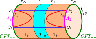
Figure 1: The subsystem $A=A_{1}\cup A_{2}$ and the corresponding candidates of the minimal surface, when $A_{2}$ is on the boundary of $1_{+-}$. Red lines: the “disconnected” surface (eq.(6)). Blue lines: one of the “connected” surfaces across the horizon (eq.(7), $n=0$). Although the time direction is not drawn here, those lines do not live on the same time slice in general.

According to the minimal area prescription Ryu and Takayanagi (2006a, b), the corresponding entanglement entropy is given by

$$S_{A} =\min\left\{S_{A}^{(c)}\,,S_{A}^{(d)}\right\}\,,$$ (5)

$$S_{A}^{(d)} =L^{(0)}(P_{1},Q_{1})+L^{(0)}(P_{2},Q_{2})\,,$$ (6)

$$S_{A}^{(c)} =\min\left\{\left.L^{(n)}(P_{1},P_{2})+L^{(n)}(Q_{1},Q_{2})\right|n\in\mathbb{Z}\right\}\,,$$ (7)

where we set $4G_{N}=1$ for simplicity. These $S_{A}^{(d)}$ and $S_{A}^{(c)}$ correspond to different topologies of the minimal surface drawn in Figure 1 by red (“disconnected”) and blue (“connected”) lines. Physical quantity

$$I(A_{1},A_{2})=S_{A_{1}}+S_{A_{2}}-S_{A}\,,$$ (8)

plays the role of the order parameter which distinguishes these two phases. That is, the red disconnected surface corresponds to $I(A_{1},A_{2})=0$ phase while the blue connected one is $I(A_{1},A_{2})>0$ phase, and it is a sharp phase transition only in the classical approximation, i.e., large $N$ on the CFT side Headrick (2010); Hartman and Maldacena (2013).

The entanglement entropy of the disconnected phase $S_{A}^{(d)}$ (6) can be written as

$$S_{A}^{(d)}= \log[\sinh(\pi T_{-}\ell_{1})\sinh(\pi T_{+}\ell_{1})\sinh(\pi T_{-}\ell_{2})\sinh(\pi T_{+}\ell_{2})]$$

$$-2\log(\pi^{2}T_{+}T_{-})+2\log{r_{\infty}^{2}}\,,$$ (9)

regardless of which boundary $A_{2}$ lives on. In particular, when the black hole is nearly extremal, we have $T_{+}^{-1}\gg\ell_{i}$ and then

$$S_{A}^{(d)}\simeq\, \log[\sinh(\pi T_{-}\ell_{1})\sinh(\pi T_{-}\ell_{2})]+\log(\ell_{1}\ell_{2})$$

$$-2\log{(\pi T_{-})}+2\log{r_{\infty}^{2}}\,.$$ (10)

IV.1 $(1_{++},1_{+-})$

First let us put $A_{2}$ in Region $1_{+-}$. This is what corresponds to the setup investigated in Hartman and Maldacena (2013). Let us take

$$\phi_{2}-\phi_{1}=\delta\phi\,,\quad\ell_{2}-\ell_{1}=\delta\ell\,.\quad t_{2}-t_{1}=\delta t\,,$$ (11)

Since the time coordinate $t$ flows to opposite directions between $1_{++}$ and $1_{+-}$ regions, we regard this $\delta t$ as the time flow of the total system. From Table  2, we obtain

$$S_{A}^{(c)} =\log X_{n}^{P}+\log X_{n}^{Q}-2\log(\pi^{2}T_{+}T_{-})+2\log{r_{\infty}^{2}}\,,$$

$$X_{n}^{P} =\cosh(\pi T_{-}(\delta\phi-\delta t+2\pi n))$$

$$\quad\times\cosh(\pi T_{+}(\delta\phi+\delta t+2\pi n))\,,$$

$$X_{n}^{Q} =\cosh(\pi T_{-}(\delta\phi-\delta t+\delta\ell+2\pi n))$$

$$\quad\times\cosh(\pi T_{+}(\delta\phi+\delta t+\delta\ell+2\pi n))\,.$$ (12)

Of course, when $T_{-}=T_{+}$, $\delta\phi=\delta\ell=0$ and $n=0$, this reproduces the corresponding result in Hartman and Maldacena (2013) (eq.(3.32)).

Furthermore, one can show that

$$S_{A}^{(c)}>4\pi T_{+}{\left|\delta t\right|}-4\log{2}-2\log{(\pi^{2}T_{+}T_{-})}+2\log{r_{\infty}^{2}}\,,$$ (13)

for arbitrary choice of $n$. Therefore in any cases, $S_{A}^{(c)}$ becomes very large in proportion to $|\delta t|$, therefore $S_{A}^{(d)}<S_{A}^{(c)}$ and $S_{A}=S_{A}^{(d)}$ in late time.

In particular, in near-extremal case, we find that the right-hand side also has a very large constant term $-2\log{T_{+}}$. It corresponds to the divergence of the distance to the horizon in the extremal black hole, which can also be observed in the case of 5D non-rotating charged extremal black hole Andrade et al. (2013). In terms of the boundary theory, it is closely related to the residual entropy, coming from IR degrees of freedom. As a result, the disconnected phase is always favored and we experience no transition in the near-extremal setup.

IV.2 $(1_{++},1_{--})$

When we put $A_{2}$ in Region $1_{+-}$ in the same way as (11), we obtain from Table  2

$$S_{A}^{(c)}= \log X_{n}^{P}+\log X_{n}^{Q}-2\log(\pi^{2}T_{+}T_{-})+2\log{r_{\infty}^{2}}\,,$$

$$X_{n}^{P}= -\sinh(\pi T_{-}(\delta\phi-\delta t+2\pi n))$$

$$\quad\times\sinh(\pi T_{+}(\delta\phi+\delta t+2\pi n))\,,$$

$$X_{n}^{Q}= -\sinh(\pi T_{-}(\delta\phi-\delta t+\delta\ell+2\pi n))$$

$$\quad\times\sinh(\pi T_{+}(\delta\phi+\delta t+\delta\ell+2\pi n))\,.$$ (14)

As we noted at the end of the previous section, these $X_{n}^{P}$ and $X_{n}^{Q}$ are not positive in general. They tend to be positive in late time for fixed values of $n$, but for any fixed time and other parameters, they become negative by taking sufficiently large $n$.

To avoid this strange property of the periodicity, let us consider a decompactifying limit and ignore the windings (i.e., set $n=0$). After fixing $n=0$, the lengths of the both geodesics are real when $\delta t>\delta t_{0}\equiv\max\{|\delta\phi|,|\delta\phi+\delta\ell|\}$. We restrict the time in this regime and consider the time evolution of the entanglement entropy after $\delta t_{0}$.

At $\delta t\to\delta t_{0}$, $S_{A}^{(c)}$ is negatively divergent. From there it increases monotonically along with $\delta{t}$, and when $\delta t$ becomes large (i.e., $\delta t\gg T_{+}^{-1},|\delta\ell|,|\delta\phi|$),

$$S_{A}^{(c)}\simeq 2{r}_{+}\delta{t}-{r}_{-}(2\delta{\phi}+\delta{\ell})-2\log(\pi^{2}{T}_{+}{T}_{-})+2\log{r}_{\infty}^{2}\,.$$ (17)

Therefore in this setup, we always experience a transition from the connected phase to the disconnected one.

IV.3 $(1_{++},1_{--})$

As we noted in section III, the boundary of $1_{-+}$ is completely timelike to that of $1_{++}$, and so it is not reasonable to consider the entanglement between $1_{++}$ and $1_{-+}$.

V Discussions

In this short letter, we discussed the entanglement in the pairs of $(1_{++},1_{+-})$ or $(1_{++},1_{--})$ boundaries, by computing the entanglement entropy of the union of two intervals $A_{1}$ and $A_{2}$. In $(1_{++},1_{+-})$ case, we have two candidates for the minimal surfaces — connected and disconnected ones —, and we can also have a freedom of the winding $n$ around the periodicity (26), for the connected surface. Phase transition between the two phases may or may not happen, depending on the parameters $T_{\pm},\delta\phi$ and $\delta\ell$. In particular, in the near-extremal regime ($T_{+}\to 0$), the disconnected phase is always favored and no transition takes place. In $(1_{++},1_{--})$ case, the story is complicated because of the counterintuitive winding modes which contribute negatively to the spacelike distance. After removing them by decompactification, we find that the phase transition always occurs.

We can also write down the entanglement entropies for $(1_{++},3_{\eta_{1}\eta_{2}})$ pairs. However, the periodicity (26) makes problems again, because it is clearly a closed timelike curve and so it is doubtful whether such sectors have physically consistent description as a field theory. Furthermore, since the boundaries of region 3 are surrounded by the conical singularities (see Figure 2 (a)), we are not sure that we can rely on the standard prescription of the minimal area surface. The naive computation itself is an easy problem by using Table  3, and we leave it to the reader.

In this letter, we analyzed the relation between entanglement and multi-boundary connected spacetime in the three dimensional bulk. It would be interesting to generalize this to higher dimensional spacetime. For deeper understanding of how generic multi-boundary spacetime are emerging related to the boundary entanglement like Maldacena and Susskind (2013), we need to find a proper interpretation or counterparts of these results in the boundary CFT. Hopefully, we would return to these problems in near future.

Appendix A Spacetime Structure of Maximally Extended Rotating BTZ

In this appendix, we briefly review the spacetime structure of the rotating BTZ black hole. Large part of the contents here was examined in Hemming et al. (2002), and we use basically the same notation as theirs.

The AdS₃ spacetime is given as an $\mathbb{R}^{2,2}$-embedded hyperboloid, expressed by

$$x_{0}^{2}+x_{1}^{2}-x_{2}^{2}-x_{3}^{2}=R^{2}\,,$$

$$ds^{2}=-dx_{0}^{2}-dx_{1}^{2}+dx_{2}^{2}+dx_{3}^{2}\,.$$ (18)

It is obvious that this space is invariant under $\mathrm{SO}(2,2)\simeq\mathrm{SL}(2,\mathbb{R})\times\mathrm{SL}(2,\mathbb{R})$, and the AdS boundary is given by

$$x_{0}^{2}+x_{1}^{2}\to\infty\,,\qquad x_{2}^{2}+x_{3}^{2}\to\infty\,.$$ (19)

We take the AdS radius $R=1$ hereafter. By introducing $U$ and $V$ as

$$U=x_{1}^{2}-x_{2}^{2}\,,\qquad V=x_{0}^{2}-x_{3}^{2}\,,$$ (20)

the AdS hyperboloid (A) represents a straight line on the $(U,V)$-plane,

$$U+V=1\,.$$ (21)

At the same time, (20) can be regarded as hyperbolae on $(x_{1},x_{2})$- and $(x_{0},x_{3})$-planes for each fixed pair $(U,V)$. That is, each point $(U,V)$ on the line (21) represents the direct product of a pair of these hyperbolae. At $(U,V)=(1,0)$ and $(0,1)$, one of these two hyperbolae becomes a pair of straight lines crossing at the origin. Note that from (21), we can decompose $(U,V)$-plane into three regions, 1: $U\geq 0,V\leq 0$, 2: $U\geq 0,V\geq 0$, and 3: $U\leq 0,V\geq 0$. This decomposition will be used later.

In this context of (20), the AdS boundary (19) corresponds to going to infinity on either (or both) of $(x_{1},x_{2})$- and $(x_{0},x_{3})$-planes along with the hyperbolae. Therefore obviously, every point $(U,V)$ on (21) touches the AdS boundary.

The BTZ black hole (1) is obtained as an orbifold,

$$\begin{pmatrix}x_{1}\\ x_{2}\\ x_{3}\\ x_{0}\end{pmatrix} \simeq\begin{pmatrix}\cosh{\gamma_{+}}&\sinh{\gamma_{+}}&0&0\\ \sinh{\gamma_{+}}&\cosh{\gamma_{+}}&0&0\\ 0&0&\cosh{\gamma_{-}}&\sinh{\gamma_{-}}\\ 0&0&\sinh{\gamma_{-}}&\cosh{\gamma_{-}}\end{pmatrix}\begin{pmatrix}x_{1}\\ x_{2}\\ x_{3}\\ x_{0}\end{pmatrix},$$

$$\gamma_{\pm} =\pm 2\pi r_{\pm}\,,$$ (22)

of the global AdS₃ spacetime (A). This orbifolded spacetime can be covered by using $12$ patches, each of which has the metric of the form of (1). Those are:

Region 1: (outside the black hole, $$r\geq r_{+}$$.)

$$x_{1} =\eta_{1}\left({\frac{r^{2}-r_{-}^{2}}{r_{+}^{2}-r_{-}^{2}}}\right)^{1/2}\cosh(\pi\left(T_{+}u^{+}+T_{-}u^{-}\right)),$$ (23b)

$$x_{2} =\eta_{1}\left({\frac{r^{2}-r_{-}^{2}}{r_{+}^{2}-r_{-}^{2}}}\right)^{1/2}\sinh(\pi\left(T_{+}u^{+}+T_{-}u^{-}\right)),$$ (23c)

$$x_{3} =\eta_{2}\left({\frac{r^{2}-r_{+}^{2}}{r_{+}^{2}-r_{-}^{2}}}\right)^{1/2}\cosh(\pi\left(T_{+}u^{+}-T_{-}u^{-}\right)),$$ (23d)

$$x_{0} =\eta_{2}\left({\frac{r^{2}-r_{+}^{2}}{r_{+}^{2}-r_{-}^{2}}}\right)^{1/2}\sinh(\pi\left(T_{+}u^{+}-T_{-}u^{-}\right))\,,$$ (23e)

Hereafter $u^{\pm}=\phi\pm t$, and the pair $(\eta_{1},\eta_{2})$ takes $(+1,+1)$, $(+1,-1)$, $(-1,+1)$, $(-1,-1)$. This region 1 covers all the sign of $x_{1}$ and $x_{3}$ in the $(U,V)$-plane with $U>0$, $V\leq 0$.

Region 2: (between the outer and inner horizons, $$r_{-}\leq r\leq r_{+}$$.)

$$x_{1} =\eta_{1}\left({\frac{r^{2}-r_{-}^{2}}{r_{+}^{2}-r_{-}^{2}}}\right)^{1/2}\cosh(\pi\left(T_{+}u^{+}+T_{-}u^{-}\right)),$$ (24b)

$$x_{2} =\eta_{1}\left({\frac{r^{2}-r_{-}^{2}}{r_{+}^{2}-r_{-}^{2}}}\right)^{1/2}\sinh(\pi\left(T_{+}u^{+}+T_{-}u^{-}\right)),$$ (24c)

$$x_{3} =\eta_{2}\left({\frac{r_{+}^{2}-r^{2}}{r_{+}^{2}-r_{-}^{2}}}\right)^{1/2}\sinh(\pi\left(T_{+}u^{+}-T_{-}u^{-}\right)),$$ (24d)

$$x_{0} =\eta_{2}\left({\frac{r_{+}^{2}-r^{2}}{r_{+}^{2}-r_{-}^{2}}}\right)^{1/2}\cosh(\pi\left(T_{+}u^{+}-T_{-}u^{-}\right)),$$ (24e)

This region 2 covers $U\geq 0$, $V\geq 0$ in the $(U,V)$-plane. Note that from region 1 to region 2, the range of $r$ changes from $r\geq r_{+}$ to $r\leq r_{+}$, and the sign of $V=x_{0}^{2}-x_{3}^{2}$ changes, while the sign of $U=x_{1}^{2}-x_{2}^{2}$ unchanged. This explains the $r-$dependent factor changes and the “$\sinh$”-“$\cosh$” flip between (23d) and (24d), and between (23e) and (24e).

Region 3: (inside the inner horizon, $$r\geq r_{+}$$.)

$$x_{1} =\eta_{1}\left({\frac{r^{2}-r_{+}^{2}}{r_{+}^{2}-r_{-}^{2}}}\right)^{1/2}\sinh(\pi\left(T_{+}u^{+}-T_{-}u^{-}\right)),$$ (25b)

$$x_{2} =\eta_{1}\left({\frac{r^{2}-r_{+}^{2}}{r_{+}^{2}-r_{-}^{2}}}\right)^{1/2}\cosh(\pi\left(T_{+}u^{+}-T_{-}u^{-}\right)),$$ (25c)

$$x_{3} =\eta_{2}\left({\frac{r^{2}-r_{-}^{2}}{r_{+}^{2}-r_{-}^{2}}}\right)^{1/2}\sinh(\pi\left(T_{+}u^{+}+T_{-}u^{-}\right)),$$ (25d)

$$x_{0} =\eta_{2}\left({\frac{r^{2}-r_{-}^{2}}{r_{+}^{2}-r_{-}^{2}}}\right)^{1/2}\cosh(\pi\left(T_{+}u^{+}+T_{-}u^{-}\right)).$$ (25e)

This region 3 covers $U\leq 0$, $V>0$ in the $(U,V)$-plane. Note that region 1 and region 3 are related by $U(=x_{1}^{2}-x_{2}^{2})$ and $V(=x_{0}^{2}-x_{3}^{2})$ exchange, therefore, region 1’s $(x_{1},x_{2},x_{3},x_{0})$ and region 3’s $(x_{0},x_{3},x_{2},x_{1})$ are exchanged.

Depending on these signs, we refer each of the $12$ regions as $1_{++}$, $2_{+-}$, etc. It can be easily shown that each of the embeddings (23)(24)(25) leads to the same induced metric (1), while the orbifold (A) becomes

$$\phi \simeq\phi+2\pi \text{(for region 1,2)}\,,$$ (26a)

$$t \simeq t+2\pi \text{(for region 3)}\,.$$ (26b)

Due to the $t\simeq t+2\pi$ identification in region 3, there is a conical singularity at the radius $r=\sqrt{r_{+}^{2}+r_{-}^{2}}$, where $g_{tt}=0$ in region 3. The Penrose diagram for this spacetime can be drawn as Figure 2 (a).

Since every point $(U,V)$ reaches to the AdS boundary, the AdS boundary is also divided into the $12$ different regions $1_{\eta_{1}\eta_{2}}$, $2_{\eta_{1}\eta_{2}}$ and $3_{\eta_{1}\eta_{2}}$, although the region 2 becomes just straight-lines on the boundary. The arrangements of $1_{\eta_{1}\eta_{2}}$ and $3_{\eta_{1}\eta_{2}}$ on the AdS global coordinate boundary, can be seen, from $\left.\tan\left(\frac{\theta\pm\tau}{2}\right)\right|_{\mu\to\infty}=\left.\left(\tanh\left(\pi T_{\pm}u_{\pm}\right)\right)^{\eta_{1}\eta_{2}}\right|_{r\to\infty}$ for region 1, and $\left.\tan\left(\frac{\theta\pm\tau}{2}\right)\right|_{\mu\to\infty}=\left.\left(\pm\tanh\left(\pi T_{\pm}u_{\pm}\right)\right)^{\mp\eta_{1}\eta_{2}}\right|_{r\to\infty}$ for region 3. The fact that $|\tanh\left(\pi u_{\pm}T_{\pm}\right)|\leq 1$ gives the restriction for the allowed parameter range in the $(\theta,\tau)$ plane, and determines whether each boundary point belongs to region $1_{\eta_{1}\eta_{2}}$, or region $3_{\eta_{1}\eta_{2}}$. The configurations of each region on the AdS boundary is drawn in Figure 2 (b).

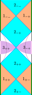
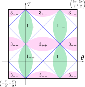
(a)		(b)

Figure 2: (a) The Penrose diagram of the rotating BTZ black hole with a two-dimensional $(t,r)$ plane set by $d\phi=N(r)dt$. Dashed lines represent BTZ (conical) singularity.
(b) The boundary in terms of global coordinate $(\theta,\tau)$, where $\theta$, $\tau$ have $2\pi$ periodicity. BTZ identifications (26) restricts the fundamental domains as the colored areas. The diagonal blue lines represent region 2.
(These two figures are essentially copies of Fig.4 and Fig.5 in Hemming et al. (2002), respectively.)

Appendix B Analytic Continuations

The different patches (23)(24)(25) can be connected to one another, by various analytic continuations of $(t,\phi,r)$ or $(u^{\pm},r)$ coordinates to complex-valued regions. The list of the ones from $1_{++}$ to $1_{\eta_{1}\eta_{2}}$ is given in Table  1. For completeness, we list the other formula of analytic continuations in Table  3.

	$u^{+}$	$u^{-}$	$r$
$2_{++}$	$u^{+}-{\frac{i}{4T_{+}}}$	$u^{-}+{\frac{i}{4T_{-}}}$	$r$
$2_{--}$	$u^{+}+{\frac{3i}{4T_{+}}}$	$u^{-}+{\frac{i}{4T_{-}}}$	$r$
$2_{+-}$	$u^{+}+{\frac{i}{4T_{+}}}$	$u^{-}-{\frac{i}{4T_{-}}}$	$r$
$2_{-+}$	$u^{+}-{\frac{3i}{4T_{+}}}$	$u^{-}-{\frac{i}{4T_{-}}}$	$r$
$3_{++}$	$u^{+}-{\frac{i}{2T_{+}}}$	$-u^{-}$	$i\sqrt{r^{2}-(r_{+}^{2}+r_{-}^{2})}$
$3_{--}$	$u^{+}+{\frac{i}{2T_{+}}}$	$-u^{-}$	$i\sqrt{r^{2}-(r_{+}^{2}+r_{-}^{2})}$
$3_{+-}$	$u^{+}$	$-u^{-}-{\frac{i}{2T_{-}}}$	$i\sqrt{r^{2}-(r_{+}^{2}+r_{-}^{2})}$
$3_{-+}$	$u^{+}$	$-u^{-}+{\frac{i}{2T_{-}}}$	$i\sqrt{r^{2}-(r_{+}^{2}+r_{-}^{2})}$

Table 3: Analytic continuations from $1_{++}$ to $2_{\eta_{1}\eta_{2}}$ and $3_{\eta_{1}\eta_{2}}$, up to the periodicity $(u^{+},u^{-})\simeq(u^{+}+i/T_{+},u^{-}\pm i/T_{-})$. In region 2, we promise that $(r^{2}-r_{+}^{2})^{1/2}=i(r_{+}^{2}-r^{2})^{1/2}$.