Mapping eQTL networks with
mixed graphical Markov models

Abstract

Expression quantitative trait loci (eQTL) mapping constitutes a challenging problem due to, among other reasons, the high-dimensional multivariate nature of gene-expression traits. Next to the expression heterogeneity produced by confounding factors and other sources of unwanted variation, indirect effects spread throughout genes as a result of genetic, molecular and environmental perturbations. From a multivariate perspective one would like to adjust for the effect of all of these factors to end up with a network of direct associations connecting the path from genotype to phenotype. In this paper we approach this challenge with mixed graphical Markov models, higher-order conditional independences and $q$-order correlation graphs. These models show that additive genetic effects propagate through the network as function of gene-gene correlations. Our estimation of the eQTL network underlying a well-studied yeast data set leads to a sparse structure with more direct genetic and regulatory associations that enable a straightforward comparison of the genetic control of gene expression across chromosomes. Interestingly, it also reveals that eQTLs explain most of the expression variability of network hub genes.

Short running title: Mapping eQTL networks with mixed GMMs

Key words: eQTL, gene network, exact likelihood ratio test, conditional Gaussian distribution, mixed graphical Markov model

Corresponding author:	Robert Castelo
	GRIB-UPF-PRBB
	Dr. Aiguader 88
	E-08003 Barcelona
	Spain
	Telf.: + 34 933 160 514
	Email: robert.castelo@upf.edu

Introduction

The simultaneous assay of gene-expression profiling and genotyping on the same samples with high-throughput technologies provides one of the primary types of integrative genomics data sets, the so-called genetical genomics data (Jansen and Nap 2001). First studies producing such data showed that, for many genes, gene expression is an heritable trait (Brem et al. 2002). Following this observation, it soon became evident that gene expression may act as an intermediate data tier that can potentially increase our power to map the genetic component of phenotypic variability in complex traits, such as human disease (Schadt et al. 2003). The genetic variants associated with each of these thousands of molecular phenotypes are known as expression quantitative trait loci (eQTL) and they can be broadly categorized into cis-acting and trans-acting associations, depending on their location relative to the gene whose expression levels map to the eQTL. Because the relative concentration of RNA molecules reflects functional relationships between genes, overlaying the correlation structure of gene expression on the eQTL associations provides an eQTL network which can help to approach the problem of reverse engineering the genotype-phenotype map with natural variation (Rockman 2008).

A straightforward way to map eQTL networks to the genome is by treating gene expression profiles as independent continuous traits and applying classical QTL mapping techniques such as single marker regression (Tesson and Jansen 2009). However, differently than higher-level phenotypes such as disease onset, adult height or yeast growth rates, gene expression is a high-dimensional multivariate trait involving measurements from thousands of genes coordinately acting under complex molecular regulatory programs. This feature makes eQTL mapping a challenging problem for, at least, two reasons. One is that gene expression profiles can be highly correlated as a product of gene regulation, thereby complicating the distinction between direct and indirect effects when marginally inspecting eQTL associations that only involve one gene at a time. The other is that high-throughput expression profiling can be very sensitive to nonbiological factors of variation such as batch effects (Leek and Storey 2007; Leek et al. 2010), introducing heterogeneity and spurious correlations between gene expression measurements. These artifacts may compromise the statistical power to map truly biological eQTLs (Stegle et al. 2010) or show up as interesting genetic switches with broad pleiotropic effects affecting a large number of genes, commonly known as eQTL hotspots (Leek and Storey 2007; Breitling et al. 2008). These problems can be addressed by estimating and including the confounding factors in the model as main (Leek and Storey 2007; Stegle et al. 2010) or mixed effects (Kang et al. 2008; Listgarten et al. 2010) and restricting the eQTL search to cis-acting variants located in the regulatory regions of the gene to which they are associated (Montgomery et al. 2010).

Yet, trans-acting eQTL have proven to be crucial to our understanding of complex regulatory mechanisms. A canonical example is locus control regions (Li et al. 2002) that enhance the expression of distal genes under tissue-specific conditions such as the one affecting the human $\beta$-globin locus. Recent contributions have shown that trans-acting mechanisms often mediate the genetic basis of disease (Westra et al. 2013).

The importance of identifying nonspurious trans-acting eQTLs has been widely recognized and a large number of approaches that aim to address the problems described above exist in the literature. They can be broadly categorized into those extending univariate single marker regression models to adjust for confounding effects (Leek and Storey 2007; Stegle et al. 2010; Listgarten et al. 2010) and those using multivariate approaches. The latter can be further categorized into Bayesian networks using conditional mutual information with constraint-based algorithms (Zhu et al. 2004), empirical Bayes hierarchical mixtures (Kendziorski et al. 2006), directed versions of the PC algorithm (Chaibub Neto et al. 2008), structural equation models (Liu et al. 2008), sparse partial least squares (Chun and Keleş 2009), fused lasso regression methods (Kim and Xing 2009), random forests (Michaelson et al. 2010), mixed Bayesian networks using the Bayesian information criterion (BIC) with homogeneous conditional Gaussian regression models (Chaibub Neto et al. 2010), mixed graphical Markov models restricted to tree network topologies (Edwards et al. 2010), sparse factor analysis (Parts et al. 2011), and conditional independence tests of order one (Bing and Hoeschele 2005; Chen et al. 2007; Kang et al. 2010; Chaibub Neto et al. 2013).

Mixed graphical Markov models and conditional independence constitute a natural extension of classical QTL mapping to multivariate phenotype vectors. This enables a smooth transition from mapping single phenotypes to building eQTL networks providing an easier statistical interpretation of the resulting associations. However, a main shortcoming of currently available methods based on mixed graphical Markov models and conditional independence is that they are restricted to conditioning on one other gene to disentangle direct and indirect relationships.

Using higher-order conditional independences on high-dimensional data, such as the one produced by genetical genomics experiments, is not trivial. The main purpose of this article is twofold: first, to show a way to use higher-order conditional independence and mixed graphical Markov models in eQTL mapping by means of $q$-order correlation graphs, and second, to demonstrate that this approach can help to obtain valuable insight into the genetic regulatory architecture of gene expression in yeast.

Materials and Methods

Expression measurements and genotyping

Throughout this article we use a well-studied genetical genomics data set generated from two yeast strains, a wild-type (RM11-1a) and a lab strain (BY4716) that were crossed to generate 112 segregants, which were genotyped and whose gene expression was profiled using two-channel microarray chips, including a dye-swap (Brem and Kruglyak 2005). We applied background correction, discarded control probes and normalized the raw expression data within and between arrays using the limma package (Smyth and Speed 2003; Ritchie et al. 2007). To correct for possible dye effects, we averaged the normalized expression values of the dye-swapped arrays. This first set of normalized data consisted of 6,216 genes and 2,906 genotype markers, i.e., a total of $p=9,122$ features, by $n=112$ samples.

Using the geno.table() and findDupMarkers() functions from the R/qtl package (Broman et al. 2003) we identified 274 markers with $>5$% missing genotypes and 749 markers with duplicated genotypes in other 260 markers. These 274+749=1,023 markers were discarded from further analysis. Among the remaining 1,883 we discarded 26 showing Mendelian segregation distortion at Holm’s FWER $<0.01$. We also removed 75 genes that could not be found in the March 2014 version of the sgdGene annotation table for the sacCer3 version of the yeast genome at the UCSC Genome Browser (http://www.genome.ucsc.edu). These filtering steps resulted in a final data set of 1,857 markers and 6,141 genes, i.e., a total of $p=7,998$ features, by $n=112$ samples. Missing genotypes were treated by complete-case analysis. The use of marginal distributions in the next section enables this approach.

Software and reproducibility

The algorithms described in this article are implemented in the open source R/Bioconductor package qpgraph available for download at http://www.bioconductor.org. Scripts with the R code reproducing the results of this article are available at http://functionalgenomics.upf.edu/supplements/eQTLmixedGMMs.

Mixed Graphical Markov models of eQTL networks

We assumed that gene expression forms a $p$-multivariate sample following a conditional Gaussian distribution given the joint probability of all genetic variants. Under this assumption a sensible model for an eQTL network is a mixed graphical Markov model -GMM- (Lauritzen and Wermuth 1989). A mixed GMM enables the integration of the joint distribution of discrete genotypes with the joint distribution of continuous expression measurements in a single multivariate statistical model satisfying a set of restrictions of conditional independence encoded by means of a graph; see (Lauritzen 1996; Edwards 2000) for a comprehensive description of this type of statistical model.

Here, we review part of the mixed GMM theory required for this paper. Mixed GMMs are statistical models representing probability distributions involving discrete random variables (r.v.’s), denoted by $I_{\delta}$ with $\delta\in\Delta$, and continuous r.v.’s, denoted by $Y_{\gamma}$ with $\gamma\in\Gamma$. This class of GMMs are determined by marked graphs $G=(V,E)$ with $p$ marked vertices $V=\Delta\cup\Gamma$, and edge set $E\subseteq V\times V$. Vertices $\delta\in\Delta$ are depicted by solid circles, $\gamma\in\Gamma$ by open ones and the entire set of them, $V$, index the vector of r.v.’s $X=(I,Y)$. In our context, continuous r.v.’s $Y$ correspond to genes and discrete r.v.’s $I$ to markers or eQTLs; see Figure 1A for a graphical representation of one such mixed GMM. We denote the joint sample space of $X$ by

$$x=(i,y)=\left\{(i_{\delta})_{\delta\in\Delta},(y_{\gamma})_{\gamma\in\Gamma}\right\}\,,$$ (1)

where $i_{\delta}$ are discrete values corresponding to genotype alleles from the marker or eQTL $I_{\delta}$ and $y_{\gamma}$ are continuous values of expression from gene $Y_{\gamma}$. The set of all possible joint discrete levels $i$ is denoted as $\mathcal{I}$. Following (Lauritzen and Wermuth 1989), we assume that the joint distribution of the variables $X$ is conditional Gaussian (also known as CG-distribution) with density function:

$$f(x)=f(i,y)=p(i)|2\pi\Sigma(i)|^{-\frac{1}{2}}\times\exp\left\{-\frac{1}{2}(y-\mu(i))^{T}\Sigma(i)^{-1}(y-\mu(i))\right\}\,.$$ (2)

This distribution has the property that continuous variables follow a multivariate normal distribution $\mathcal{N}_{|\Gamma|}(\mu(i),\Sigma(i))$ conditioned on the discrete variables. The parameters $\left(p(i),\mu(i),\Sigma(i)\right)$ are called moment characteristics where $p(i)$ is the probability that $I=i$, and $\mu(i)$ and $\Sigma(i)$ are the conditional mean and covariance matrix of $Y$ which depend on joint discrete level $i$. If the covariance matrix is constant across the levels of $\mathcal{I}$, that is, $\Sigma(i)\equiv\Sigma$, the model is homogeneous. Otherwise, the model is said to be heterogeneous. Throughout this article we assume an homogeneous mixed GMM underlying the eQTL network. This implies that genotypes affect only the mean expression level of genes and not the correlations between them. We can write the logarithm of the density in terms of the canonical parameters $(g(i),h(i),K(i))$:

$$\log f(i,y)=g(i)+h(i)^{T}y-\frac{1}{2}y^{T}K(i)y\,,\;\;$$ (3)

where

$$g(i) = \log(p(i))-\frac{1}{2}\log|\Sigma(i)|-\frac{1}{2}\mu(i)^{T}\Sigma(i)^{-1}\mu(i)-\frac{|\Gamma|}{2}\log(2\pi)\,,$$ (4)

$$h(i) = \Sigma(i)^{-1}\mu(i)\,,$$ (5)

$$K(i) = \Sigma(i)^{-1}\,.$$ (6)

CG-distributions satisfy the Markov property if and only if their canonical parameters are expanded into interaction terms such that only interactions between adjacent vertices are present (Lauritzen 1996). Thus,

$$g(i)=\!\sum_{d\subseteq\Delta}\lambda_{d}(i)\,,\quad h_{\gamma}(i)=\!\sum_{d\subseteq\Delta}\eta_{d}(i)_{\gamma},\quad k_{\gamma\eta}(i)=\!\sum_{d\subseteq\Delta}\psi_{d}(i)_{\gamma\eta}\;,$$ (7)

where $\lambda_{d}(i)>0$, with $d\subseteq\Delta$ complete in $G$, represent the discrete interactions among the variables indexed by $d$; $\eta_{d}(i)_{\gamma}>0$, with $d\cup\{\gamma\}$ complete in $G$, represent the mixed interactions between $X_{\gamma}$ and the variables indexed by $d$; and $\psi_{d}(i)_{\gamma\eta}>0$, with $d\cup\{\gamma,\eta\}$ complete in $G$, represent the quadratic interactions between $X_{\gamma},X_{\eta}$ and the variables indexed by $d$. If the model is homogeneous, there are no mixed quadratic interactions, i.e., $\psi_{d}(i)_{\gamma\eta}=0$ for $d\neq\emptyset$. Plugging these expansions in Eq. (3) we obtain

$$\log f(i,y)=\sum_{d\subseteq\Delta}\lambda_{d}(i)+\sum_{d\subseteq\Delta}\sum_{\gamma\in\Gamma}\eta_{d}(i)_{\gamma}y_{\gamma}-\frac{1}{2}\sum_{d\subseteq\Delta}\sum_{\gamma,\eta\in\Gamma}\psi_{d}(i)_{\gamma\eta}y_{\gamma}y_{\eta}\,.$$ (8)

Decomposable mixed GMMs: An important subclass of mixed GMMs is defined by decomposable marked graphs. A triple $(A,B,C)$ of disjoint subsets of $V$ form a decomposition of an undirected marked graph $G$ if $V=A\cup B\cup C$ and: (1) $C$ is a complete subset of $V$; (2) $C$ separates $A$ from $B$; and (3) $C\subseteq\Delta$ or $B\subseteq\Gamma$. An undirected marked graph $G$ is said to be decomposable if it is complete, or if there exists a proper decomposition $(A,B,C)$ such that the subgraphs $G_{A\cup C}$ and $G_{B\cup C}$ are decomposable. In different terms, when $G$ is undirected, decomposability of $G$ holds if and only if $G$ does not contain chordless cycles of length larger than 3 and does not contain any path between two non-adjacent discrete vertices passing through continuous vertices only.

Maximum Likelihood Estimates of mixed GMMs: Let ${\cal X}=\{x^{\left(\nu\right)}\}=\{\left(i^{\left(\nu\right)},y^{\left(\nu\right)}\right)\}$ be a sample of $\nu=1,...,n$ independent and identically distributed observations from a CG-distribution. For an arbitrary subset $A\subseteq V$, we abbreviate to $i_{A}=i_{A\cap\Delta}$, $\mathcal{I}_{A}=\mathcal{I}_{\Delta\cap A}$ and $y_{A}=y_{A\cap\Gamma}$ and the following sampling statistics are defined:

$$n(i)\!\! = \!\!\#\left\{\nu:i^{(\nu)}\!=i\right\}\,,$$ (9)

$$s(i)\!\! = \!\!\sum\limits_{\nu:i^{(\nu)}=i}y^{(\nu)}\,,$$ (10)

$$\bar{y}(i)\!\! = \!\!s(i)/n(i)\,,$$ (11)

$$ss(i)\!\! = \!\!\sum\limits_{\nu:i^{(\nu)}=i}y^{(\nu)}(y^{(\nu)})^{T}\,,$$ (12)

$$ssd(i)\!\! = \!\!ss(i)-s(i)s(i)^{T}/n(i)\,,$$ (13)

$$ssd_{A}(A)\!\! = \!\!\sum_{i_{A}\in\mathcal{I}_{A}}ssd_{A\cap\Gamma}(i_{A})\,.$$ (14)

The likelihood function for the homogeneous, saturated model attains its maximum if and only if $n\geq|\Gamma|+|\mathcal{I}|$, which is almost surely equal to $n(i)>0$ for all $i\in\mathcal{I}$ (Lauritzen 1996, Prop. 6.10). In such a case the maximum likelihood estimates (MLEs) of the moment characteristics are defined as

$$\hat{p}(i)=n(i)/n,\quad\hat{\mu}(i)=\bar{y}(i),\quad\hat{\Sigma}=ssd_{V}(V)/n=ssd/n\,.$$ (15)

It follows, then, that saturated mixed GMMs cannot be directly estimated from data with $p\gg n$, using only the formulas described above. For the unsaturated case, decomposable mixed GMMs also admit explicit MLEs. In the homogeneous decomposable case it can be shown (Lauritzen 1996, Prop. 6.21) that the MLE exists almost surely if and only if $n(i_{C})\geq|C\cap\Gamma|+|\mathcal{I}_{C}|$ for all cliques $C$ of $G$ and $i_{C}\in\mathcal{I}_{C}$. In this case, MLEs are defined with the following canonical parameters (Lauritzen 1996, pg. 189):

$$\hat{p}(i) =\prod_{j=1}^{k}\frac{n(i_{C_{j}})}{n(i_{S_{j}})}\,,$$ (16)

$$\hat{h}(i) =n\Biggl{\{}\sum_{j=1}^{k}\left[ssd_{C_{j}}(C_{j})^{-1}\bar{y}_{C_{j}}(i_{C_{j}})\right]^{|\Gamma|}-\left[ssd_{S_{j}}(S_{j})^{-1}\bar{y}_{S_{j}}(i_{S_{j}})\right]^{|\Gamma|}\Biggr{\}}\,,$$ (17)

$$\hat{K} =n\Biggl{\{}\sum_{j=1}^{k}\!\left[ssd_{C_{j}}(C_{j})^{-1}\right]^{|\Gamma|}\!\!-\!\!\left[ssd_{S_{j}}(S_{j})^{-1}\right]^{|\Gamma|}\Biggr{\}}\,,$$ (18)

where $S_{1}=\emptyset$. The matrices $[M]^{|\Gamma|}$ of Eq. (18) are defined as follows. Given a matrix $M=\{m_{\gamma\eta}\}_{|A|\times|A|}$ of dimension $|A|\times|A|$ with $A\subseteq\Gamma$, $[M]^{|\Gamma|}$ is a $|\Gamma|\times|\Gamma|$ matrix such that

$$[M]_{\gamma\eta}^{|\Gamma|}=\begin{cases}m_{\gamma\eta},&\text{if $\{\gamma,\eta\}\in A$}\,,\\ 0,&\text{otherwise}\,.\end{cases}$$

Analogously, in Eq. (17), $[M]^{|\Gamma|}$ is a $|\Gamma|$-length vector obtained from a $|A|$-length vector $M$.

Simulation of eQTL network models with mixed GMMs

In this subsection, we describe how to simulate eQTL networks with homogeneous mixed GMMs and data from them. We restrict ourselves to the case of a backcross, in which each genotype marker can have two different alleles AA and AB. However, these procedures could be extended to more complex cross models allowing for other than linear additive effects (codominant model) on the mixed associations, such as dominance effects.

Simulation of eQTL network structures: The first step to simulate a GMM consists of simulating its associated graph $G=(V,E)$ that defines the structure of the eQTL network. eQTLs and expression profiles are represented in $G$ by discrete vertices $\Delta$ and continuous vertices $\Gamma$, respectively, such that $V=\Delta\cup\Gamma$ and $|V|=p$. In the context of genetical genomics data we make the assumption that discrete genotypes affect gene-expression measurements and not the other way around. Thus, we consider the underlying graph $G$ as a marked graph where some edges are directed and represented by arrows and some are undirected. More concretely, $G$ will have arrows pointing from discrete vertices to continuous ones, undirected edges between continuous vertices and no edges between discrete vertices. From this restriction, it follows that there are no semi-directed cycles and allows one to interpret these GMMs as chain graphs, which are graphs formed by undirected subgraphs connected by directed edges (Lauritzen 1996).

Simulation of parameters of a homogeneous mixed GMM: Here we show how to simulate the parameters of the homogeneous CG-distribution represented by $G$ with given marginal linear correlations of magnitude $\rho$ on the pure continuous (gene-gene) associations and given additive effects of magnitude $a$ on the mixed (eQTL) ones.

Covariance matrix. Given the structure of a graph $G$, a random covariance matrix $\Sigma$ can be simulated as follows. Let $G_{\Gamma}\subseteq G$ denote the subgraph of $p_{\Gamma}=|\Gamma|$ pure continuous vertices and let $\rho$ denote the desired mean marginal correlation between each pair of continuous r.v.’s $(X_{\gamma},X_{\eta})$ such that $(\gamma,\eta)\in G_{\Gamma}$. Let ${\cal S}^{+}(G_{\Gamma})\subset{\cal S}^{+}$ denote the set of all $p_{\Gamma}\times p_{\Gamma}$ positive definite matrices in ${\cal S}^{+}$ such that every matrix $S\in{\cal S}^{+}(G_{\Gamma})$ satisfies that $\{S^{-1}\}_{ij}=0$ whenever $i\neq j$ and $(i,j)\not\in G_{\Gamma}$.

We simulate $\Sigma$ such that $\Sigma\in{\cal S}^{+}(G_{\Gamma})$ in two steps. First, we build an initial positive definite matrix $\tilde{\Sigma}_{0}\in{\cal S}^{+}$ and, from this, we build the incomplete matrix $\Sigma_{0}$ with elements $\{\sigma_{ij}^{0}\}$ if either $i=j$ or $(i,j)\in G_{\Gamma}$, and the remaining elements unspecified. Second, we search for a positive completion of $\Sigma_{0}$, which consists of filling up $\Sigma_{0}$ in such a way that the resulting $\Sigma\in{\cal S}^{+}(G_{\Gamma})$.

It can be shown (Grone et al. 1984) that the incomplete matrix $\Sigma_{0}$ admits a positive completion and that it is unique. This means that, given $\Sigma_{0}$, we can use algorithms for maximum-likelihood estimation or Bayesian conjugate inference (Roverato 2002) as matrix completion algorithms. To this end, we first draw $\Sigma_{0}$ from a Wishart distribution $W_{p_{\Gamma}}(\Lambda,p_{\Gamma})$ with $\Lambda=D\tilde{\Sigma}_{0}D,D=\textrm{diag}(\{\sqrt{1/p_{\Gamma}}\}_{p_{\Gamma}})$ and $\tilde{\Sigma}_{0}=\{\tilde{\Sigma}_{0_{ij}}\}_{p_{\Gamma}\times p_{\Gamma}}$ where $\tilde{\Sigma}_{0_{ij}}=1$ for $i=j$ and $\tilde{\Sigma}_{0_{ij}}=\rho$ for $i\neq j$. It is required that $\Lambda\in{\cal S}^{+}$ and this happens if and only if $-1/(p_{\Gamma}-1)<\rho<1$ (Seber 2007, pg. 317). Finally, we apply the iterative regression procedure introduced by Hastie et al. (2009, pg. 634) for maximum-likelihood estimation of Gaussian GMMs with known structure, as matrix completion algorithm to obtain $\Sigma$ from $\Sigma_{0}$.

Probability of discrete levels. Since we are simulating a backcross, each discrete r.v. takes two possible values $i_{\delta}=\{1,2\}$ with equal probability $p(i_{\delta}=1)=p(i_{\delta}=2)=0.5$. For the sole purpose of simulating eQTL networks we made the simplifying assumption that discrete r.v.’s representing eQTLs are marginally independent between them. From these two assumptions it follows that joint levels $i\in\mathcal{I}$ are uniformly distributed, that is, $p(i)=1/|\mathcal{I}|$, $\forall i\in\mathcal{I}$.

Conditional mean vector. Let a discrete variable $I_{\delta}$ have an additive effect $a_{\delta\gamma}$ on the continuous variable $Y_{\gamma}$. In the case of a backcross this implies that:

$$a_{\delta\gamma}=\mu_{\gamma}(1)-\mu_{\gamma}(2)=\frac{1}{|\mathcal{I}|/2}\sum_{i^{\prime}:i_{\delta}=1}\mu(i^{\prime})-\frac{1}{|\mathcal{I}|/2}\sum_{i^{\prime}:i_{\delta}=2}\mu(i^{\prime})\,.$$ (19)

Using Eq. (5) we can calculate the conditional mean vector as $\mu(i)=\Sigma\cdot h(i)$. This enables simulating the covariance matrix independently from discrete r.v.’s while interpreting it as a conditional one to generate $\mu(i)$. The values of the canonical parameter $h(i)=\{h_{\gamma}(i)\}_{\gamma\in\Gamma}$ determine the strength of the mixed interactions between discrete and continuous r.v.’s. Using Eq. (7) they can be calculated as follows:

$$h_{\gamma}(i)=\begin{cases}\eta_{\emptyset\gamma},&\text{if $(\delta,\gamma)\not\in E$ $\forall\delta\in\Delta$}\,,\\ \{\eta_{\delta}(i_{\delta})_{\gamma}\}_{i_{\delta}\in\mathcal{I}_{\delta}}=\{\eta_{\delta}(1)_{\gamma},\eta_{\delta}(2)_{\gamma}\},&\text{if $(\delta,\gamma)\in E$, $\delta\in\Delta$}\,.\end{cases}$$

Without loss of generality, values $\eta_{\emptyset\gamma}$ are set to zero. To set values $\eta_{\delta}(1)_{\gamma}$ and $\eta_{\delta}(2)_{\gamma}$, so that both Eqs. (5) and (19) are satisfied, we proceed as follows. Assume that an eQTL $I_{\delta}$ has a pleiotropic effect on a set of genes $\{Y_{\gamma}\}_{\gamma\in A_{\delta}}$, where $A_{\delta}=\{\gamma\in\Gamma:(\delta,\gamma)\in E\}$. By combining Eqs. (5) and (19), for each $\gamma\in A_{\delta}$ we have that

$$a_{\delta\gamma} = \frac{1}{|\mathcal{I}|/2}\sum_{i^{\prime}:i_{\delta}=1}\sum_{\zeta\in\Gamma}\sigma_{\gamma\zeta}h_{\zeta}(i^{\prime})-\frac{1}{|\mathcal{I}|/2}\sum_{i^{\prime}:i_{\delta}=2}\sum_{\zeta\in\Gamma}\sigma_{\gamma\zeta}h_{\zeta}(i^{\prime})=$$

$$= \frac{1}{|\mathcal{I}|/2}\sum_{\zeta\in\Gamma}\sigma_{\gamma\zeta}\left\{\sum_{i^{\prime}:i_{\delta}=1}h_{\zeta}(i^{\prime})-\sum_{i^{\prime}:i_{\delta}=2}h_{\zeta}(i^{\prime})\right\}\,.$$

Note that if $j,k\in\mathcal{I}$ are two discrete levels such that $j_{\delta}=1$, $k_{\delta}=2$ and $j_{\Delta\backslash\{\delta\}}=k_{\Delta\backslash\{\delta\}}$, then $h_{\zeta}(j)=h_{\zeta}(k)$ for all $\zeta\notin A_{\delta}$. It follows that for all $\zeta\notin A_{\delta}$ the terms $h_{\zeta}(i^{\prime})$ in both summations cancel out and we obtain,

$$a_{\delta\gamma} = \frac{2}{|\mathcal{I}|}\sum_{\zeta\in A_{\delta}}\sigma_{\gamma\zeta}\left\{\sum_{i^{\prime}:i_{\delta}=1}h_{\zeta}(i^{\prime})-\sum_{i^{\prime}:i_{\delta}=2}h_{\zeta}(i^{\prime})\right\}=$$

$$= \frac{2}{|\mathcal{I}|}\sum_{\zeta\in A_{\delta}}\sigma_{\gamma\zeta}\left\{\frac{|\mathcal{I}|}{2}\eta_{\delta}(1)_{\gamma}-\frac{|\mathcal{I}|}{2}\eta_{\delta}(2)_{\gamma}\right\}=\sum_{\zeta\in A_{\delta}}\sigma_{\gamma\zeta}\left\{\eta_{\delta}(1)_{\gamma}-\eta_{\delta}(2)_{\gamma}\right\}\,.$$

Let $\eta_{\delta\gamma}=\eta_{\delta}(1)_{\gamma}-\eta_{\delta}(2)_{\gamma}$ and the vectors $\boldsymbol{a}_{\delta A_{\delta}}=\{a_{\delta\gamma}\}_{\gamma\in A_{\delta}}$, $\boldsymbol{\eta}_{\delta A_{\delta}}=\{\eta_{\delta\gamma}\}_{\gamma\in A_{\delta}}$, $\boldsymbol{\eta}_{1A_{\delta}}=\{\eta_{\delta}(1)_{\gamma}\}_{\gamma\in A_{\delta}}$ and $\boldsymbol{\eta}_{2A_{\delta}}=\{\eta_{\delta}(2)_{\gamma}\}_{\gamma\in A_{\delta}}$. We write the matrix form of the previous expression as,

$$\boldsymbol{a}_{\delta A_{\delta}} = \Sigma_{\{A_{\delta},A_{\delta}\}}\boldsymbol{\eta}_{\delta A_{\delta}}\,,$$

$$\boldsymbol{\eta}_{\delta A_{\delta}} = \Sigma_{\{A_{\delta},A_{\delta}\}}^{-1}\boldsymbol{a}_{\delta A_{\delta}}\,,$$

$$\boldsymbol{\eta}_{1A_{\delta}} = \Sigma_{\{A_{\delta},A_{\delta}\}}^{-1}\boldsymbol{a}_{\delta A_{\delta}}+\boldsymbol{\eta}_{2A_{\delta}}\,.$$

Simulation of eQTL network models of experimental crosses

We have integrated the algorithms presented above with functions from the R/qtl package (Broman et al. 2003) to simulate eQTL network models of experimental crosses and data from them in the following way. First, we simulate a genetic map with a given number of chromosomes and markers using the sim.map() function of the R/qtl package.

Second, we simulate a homogeneous mixed GMM in two steps: (a) we define the, possibly random, underlying regulatory model of eQTLs and gene-gene associations; (b) we simulate the parameters $(p(i),\mu(i),\Sigma)$ of this homogeneous mixed GMM according to the procedures described above.

Third, we simulate data from the previous eQTL network model with the function sim.cross() from the R/qtl package. This function is overloaded in qpgraph to plug the eQTL associations into the corresponding genetic loci and return a R/qtl cross object. The function sim.cross() defined in the qpgraph package proceeds as follows. First, the genotype data is simulated by the procedures implemented in the R/qtl package. Genotypes are sampled at each marker from a Markov chain with transition probabilities that depend on the distance between markers and a mapping function. eQTLs are placed at the markers and, in particular, if eQTLs are located sufficiently away from each other, we can assume that the corresponding discrete r.v.’s are marginally independent between them. Finally, qpgraph simulates gene expression values according to the homogeneous mixed GMM by sampling continuous observations from the corresponding parameters of the CG-distribution $\mathcal{N}_{|\Gamma|}\left(\mu(i),\Sigma\right)$, given the sampled genotype $i$ from all joint eQTLs.

Conditional independence tests parametrized by mixed GMMs

Approaches to learning the structure of a mixed GMM using higher-order correlations require testing for conditional independence between any two r.v.’s $X_{\alpha}$ and $X_{\beta}$, such that $\beta\subseteq\Gamma$, given a set of conditioning ones $X_{Q}$, denoted by $X_{\alpha}\bot\bot X_{\beta}|X_{Q}$. To this end, we use a likelihood-ratio test (LRT) between two models: a saturated model $\mathcal{M}_{1}$, determined by the complete graph $G^{1}=\left(V,E^{1}\right)$, where $V=\{\alpha,\beta,Q\}$ and $E^{1}=V\times V$, and a constrained model $\mathcal{M}_{0}$, determined by $G^{0}=\left(V,E^{0}\right)$ with exactly one missing edge between the two vertices $\alpha,\beta$ and thus $E^{0}=\{V\times V\}\backslash\left(\alpha,\beta\right)$ and $Q=V\backslash\{\alpha,\beta\}$.

Since $G^{1}$ is complete and $\left(\alpha,\beta,Q\right)$ is a proper decomposition of $G^{0}$, $\mathcal{M}_{1}$ and $\mathcal{M}_{0}$ are both decomposable, and therefore, they admit explicit MLEs (Eqs. 16-18). Given that $V=\Delta\cup\Gamma$, we denote by $(\gamma,\zeta)$ a pair of continuous r.v.’s (i.e., $\gamma,\zeta\in\Gamma$), and by $(\delta,\gamma)$ a pair of mixed r.v.’s with $\delta\in\Delta$ and, $\gamma\in\Gamma$, so that either $Q=V\backslash\{\gamma,\zeta\}$ or $Q=V\backslash\{\delta,\gamma\}$ are the conditioning subsets.

In the context of homogeneous mixed GMMs, the null hypothesis of conditional independence for the pure continuous case, $\gamma\bot\bot\zeta|Q$, corresponds to a zero value in the $\left(\gamma,\zeta\right)$ and $\left(\zeta,\gamma\right)$ entries of the canonical parameter $K$ (see Eqs. 7, 8). The log-likelihood-ratio statistic, which is twice the difference of the log-likelihoods of models $\mathcal{M}_{0}$ and $\mathcal{M}_{1}$, is reduced to (see Lauritzen 1996, pg. 192):

$$D_{\gamma\zeta.Q}=-2\ln\left(\frac{\mathcal{L}_{0}}{\mathcal{L}_{1}}\right)=-2\ln\left(\frac{|ssd_{\Gamma}||ssd_{\Gamma\backslash\{\gamma,\zeta\}}|}{|ssd_{\Gamma\backslash\{\gamma\}}||ssd_{\Gamma\backslash\{\zeta\}}|}\right)^{n/2}=-2\ln\left(\Lambda_{\gamma\zeta.Q}\right)^{n/2}\,.$$ (20)

The null hypothesis of conditional independence in the mixed case, $\delta\bot\bot\gamma|Q$, corresponds to an expansion of the canonical parameter $h_{\gamma}(i)$ where the terms corresponding to $\delta$ are zero, $\eta_{\delta}(i)_{\gamma}=0$ (see Eqs. 7, 8). In this case, the log-likelihood-ratio statistic is (Lauritzen 1996, pg. 194):

$$D_{\delta\gamma.Q}=-2\ln\left(\frac{|ssd_{\Gamma}||ssd_{\Gamma^{*}}(\Delta^{*})|}{|ssd_{\Gamma^{*}}||ssd_{\Gamma}(\Delta^{*})|}\right)^{n/2}=-2\ln\left(\Lambda_{\delta\gamma.Q}\right)^{n/2}\,,$$ (21)

where $\Gamma^{*}=\Gamma\backslash\{\gamma\}$ and $\Delta^{*}=\Delta\backslash\{\delta\}$. Since models $\mathcal{M}_{1}$ and $\mathcal{M}_{0}$ are decomposable, they are collapsible onto the same set of variables $X_{V\backslash\{\gamma\}}$; see (Edwards 2000, pg. 86-87) and (Didelez and Edwards 2004). This property implies that the density functions $f$ of $\mathcal{M}_{1}$ and $\mathcal{M}_{0}$ can be factorized as $f_{V}=f_{V\backslash\{\gamma\}}\cdot f_{\gamma|V\backslash\{\gamma\}}$ such that the marginal and conditional densities, $f_{V\backslash\{\gamma\}}\in\mathcal{M}_{V\backslash\{\gamma\}}$ and $f_{\gamma|V\backslash\{\gamma\}}\in\mathcal{M}_{\gamma|V\backslash\{\gamma\}}$, respectively, can be parametrized separately. Therefore, the likelihood function of $\mathcal{M}_{1}$ and $\mathcal{M}_{0}$ can be computed as the product of the likelihood of the marginal and the conditional models, $\mathcal{L}_{1}=\mathcal{L}_{\gamma|V\backslash\{\gamma\}}^{1}\cdot\mathcal{L}_{V\backslash\{\gamma\}}^{1}$ and $\mathcal{L}_{0}=\mathcal{L}_{\gamma|V\backslash\{\gamma\}}^{0}\cdot\mathcal{L}_{V\backslash\{\gamma\}}^{0}$, respectively.

It follows that the second term of these factorizations corresponds to the same saturated model induced by the complete subgraph formed by the vertices in $V\backslash\{\gamma\}$, $\mathcal{L}_{V\backslash\{\gamma\}}^{1}=\mathcal{L}_{V\backslash\{\gamma\}}^{0}$, and we have that

$$D_{\gamma\zeta.Q}=-2\ln\left(\frac{\mathcal{L}_{0}}{\mathcal{L}_{1}}\right)=-2\ln\left(\frac{\mathcal{L}_{\gamma|V\backslash\{\gamma\}}^{0}}{\mathcal{L}_{\gamma|V\backslash\{\gamma\}}^{1}}\right)=-2\ln\left(\frac{\hat{\sigma}_{\gamma|V\backslash\{\gamma\}}^{0}}{\hat{\sigma}_{\gamma|V\backslash\{\gamma\}}^{1}}\right)^{-n/2}\,,$$ (22)

where $\hat{\sigma}_{\gamma|V\backslash\{\gamma\}}^{0}$ and $\hat{\sigma}_{\gamma|V\backslash\{\gamma\}}^{1}$ denote the estimates of the conditional variance of the r.v. $X_{\gamma}$ given the rest of the r.v.’s under the null and the alternative conditional models $\mathcal{M}_{\gamma|V\backslash\{\gamma\}}^{0}$ and $\mathcal{M}_{\gamma|V\backslash\{\gamma\}}^{1}$, respectively. In particular, these conditional models are equivalent to the ANCOVA models (Edwards 2000, pg. 91) in which the continuous r.v. $\gamma\in\Gamma$ is the response variable and the rest are explanatory. In this context, we have that $\hat{\sigma}_{\gamma|V\backslash\{\gamma\}}^{0}=\text{RSS}_{0}/n$ and $\hat{\sigma}_{\gamma|V\backslash\{\gamma\}}^{1}=\text{RSS}_{1}/n$, where RSS is the residual sum of squares of the corresponding ANCOVA model and $n$ is the sample size. The ANCOVA model corresponding to $\mathcal{M}_{\gamma|V\backslash\{\gamma\}}^{1}$ for the case of a backcross is,

$$X_{\gamma}=\mu+\beta_{\delta}Z_{\delta}+\sum_{\kappa\in\Delta^{*}}\beta_{\kappa}Z_{\kappa}+\sum_{\kappa_{1}=2}^{|\Delta|}\sum_{\kappa_{2}=1}^{{|\Delta|\choose\kappa_{1}}}\left[\beta_{\kappa_{1}\kappa_{2}}\left(\prod_{\kappa=1}^{\kappa_{1}}{Z}_{\kappa}\right)\right]+\sum_{\lambda\in\Gamma^{*}}\beta_{\lambda}X_{\lambda}+\epsilon\,.$$ (23)

In this model, $\mu$ is the phenotype’s mean, the term $\beta_{\delta}Z_{\delta}$ represents the effect of the discrete variable $\delta\in\Delta$ that we are testing and we assume that $\epsilon\sim\mathcal{N}\left(0,\sigma_{\gamma}^{2}\right)$. The continuous r.v.’s in $Q$, $\Gamma^{*}$, are modeled as a linear combination of r.v.’s (third summation of the equation). On the other hand, the joint levels of $\delta$ and of the discrete r.v.’s in $Q$, $\Delta$, are encoded through $(|\mathcal{I}|-1)$ terms where some of them represent the main effects of each discrete r.v. (first summation). The rest of the terms encode all the interacting effects between the discrete r.v.’s (second summation). Each variable $Z_{\kappa}$ is an indicator variable that, in the case of a backcross, takes values 0 or 1 if the genotype of $I_{\kappa}$ is AA or AB, respectively.

The count of the number of parameters in the model of Eq. (23) is as follows: $|\Delta|$ parameters come from the term encoding the main effect of $Z_{\delta}$ and the first summation; the second summation involves $2^{|\Delta|}-1-|\Delta|$ terms whereas the third one involves $|\Gamma|-1$ terms. Thus, the saturated model $\mathcal{M}_{\gamma|V\backslash\{\gamma\}}^{1}$ described in Eq. (23) has $2^{|\Delta|}+|\Gamma|-2$ free parameters in total, and therefore, $n-2^{|\Delta|}-|\Gamma|+2$ degrees of freedom, where $n$ is the sample size of the data.

For the pure continuous case, the conditional model corresponding to $\mathcal{M}_{\gamma|V\backslash\{\gamma\}}^{0}$ is the same as the one in Eq. (23) except that we remove the term of the third summation that corresponds to the variable $X_{\zeta}$. In this case, this model has $n-2^{|\Delta|}-|\Gamma|+3$ degrees of freedom. Therefore, under the null hypothesis, the statistic $D_{\gamma\zeta.Q}$ follows asymptotically a $\chi_{df}^{2}$ distribution with $df=1$ degree of freedom.

In general, we can derive the degrees of freedom for the pure continuous case by writing explicitly the conditional expectation of $X_{\gamma}$ given $X_{V\backslash\{\gamma\}}$. Under $\mathcal{M}_{\gamma|V\backslash\{\gamma\}}^{1}$ this corresponds to,

$$\textrm{E}\left(X_{\gamma}|\Delta,\Gamma\backslash\{\gamma\}\right)=\alpha(i_{\Delta})+\!\!\!\!\sum_{\lambda\in\Gamma\backslash\{\gamma\}}\!\!\!\beta_{\gamma\lambda|\Gamma\backslash\{\gamma\}}X_{\lambda}\,,$$ (24)

where $\alpha(i_{\Delta})=\mu_{\gamma}(i_{\Delta})\!-\!\sum_{\lambda\in\Gamma\backslash\{\gamma\}}\!\beta_{\gamma\lambda|\Gamma\backslash\{\gamma\}}\mu_{\lambda}(i_{\Delta})$ and $\beta_{\gamma\lambda|\Gamma\backslash\{\gamma\}}$ is the partial regression coefficient that is found through the canonical parameter $K=\{k_{\gamma\zeta}\},\forall\gamma,\zeta\in\Gamma$, as $\beta_{\gamma\lambda|\Gamma\backslash\{\gamma\}}=-k_{\gamma\lambda}/k_{\gamma\gamma}$ (Lauritzen 1996, pg. 130). This model has $n-|\mathcal{I}|-|\Gamma|+1$ degrees of freedom since it has $|\mathcal{I}|$ parameters that come from the first term in Eq. (24) and $|\Gamma|-1$ from the second term. On the other hand, the conditional expectation of $X_{\gamma}$ given $X_{V\backslash\{\gamma\}}$ under $M_{\gamma|V\backslash\{\gamma\}}^{0}$ is

$$\textrm{E}\left(X_{\gamma}|\Delta,\Gamma\backslash\{\gamma,\zeta\}\right)=\alpha(i_{\Delta})+\!\!\!\!\sum_{\lambda\in\Gamma\backslash\{\gamma,\zeta\}}\!\!\!\beta_{\gamma\lambda|\Gamma\backslash\{\gamma,\zeta\}}X_{\lambda}\,,$$

which leads to $n-|\mathcal{I}|-|\Gamma|+2$ degrees of freedom. By computing the difference in the degrees of freedom of both models, we have that $D_{\gamma\zeta.Q}$ follows asymptotically a $\chi_{df}^{2}$ distribution with $df=1$ degree of freedom.

In the mixed case, the likelihood-ratio statistic $D_{\delta\gamma.Q}$ of Eq. (21) is related to the LOD score used in QTL mapping

$$\text{LOD}=\log_{10}\left(\frac{\mathcal{L}_{1}}{\mathcal{L}_{0}}\right)\,,$$

through the following transformation of the LOD score:

$$D_{\delta\gamma.Q}=2\ln(10)\text{LOD}\,.$$ (25)

In fact, since the ratio between $\mathcal{L}_{1}$ and $\mathcal{L}_{0}$ is equivalent to the ratio between $\mathcal{L}_{\gamma|V\backslash\{\gamma\}}^{1}$ and $\mathcal{L}_{\gamma|V\backslash\{\gamma\}}^{0}$ we have that

$$\text{LOD}=\log_{10}\left(\frac{\mathcal{L}_{1}}{\mathcal{L}_{0}}\right)=\log_{10}\left(\frac{\mathcal{L}_{\gamma|V\backslash\{\gamma\}}^{1}}{\mathcal{L}_{\gamma|V\backslash\{\gamma\}}^{0}}\right)\,.$$ (26)

In this case, the conditional saturated model $\mathcal{M}_{\gamma|V\backslash\{\gamma\}}^{1}$ for a backcross is the same as the one in Eq. (23). By contrast, in the conditional constrained model $\mathcal{M}_{\gamma|V\backslash\{\gamma\}}^{0}$ we delete all the terms of Eq. (23) that involve the r.v. $X_{\delta}$. This constrained model has $n-2^{|\Delta|-1}-|\Gamma|+2$ free parameters. Thus, for a backcross the likelihood-ratio statistic $D_{\delta\gamma.Q}$, and therefore, the transformation of the LOD score (Eq. 25), follows a $\chi_{df}^{2}$ distribution with $df=2^{|\Delta|-1}$ degrees of freedom.

Again, we can derive the degrees of freedom of the $\chi^{2}_{df}$ distribution of the general case by looking at the conditional expectation of models $\mathcal{M}_{\gamma|V\backslash\{\gamma\}}^{1}$ (Eq. 24), and $\mathcal{M}_{\gamma|V\backslash\{\gamma\}}^{0}$ written as

$$\textrm{E}\left(X_{\gamma}|\Delta\backslash\{\delta\},\Gamma\backslash\{\gamma\}\right)=\alpha(i_{\Delta\backslash\{\delta\}})+\!\!\!\!\sum_{\lambda\in\Gamma\backslash\{\gamma\}}\!\!\!\beta_{\gamma\lambda|\Gamma\backslash\{\gamma\}}X_{\lambda}\,.$$ (27)

Here, the first term involves $|\mathcal{I}_{\Delta^{*}}|$ parameters and the second $|\Gamma|-1$, so that the constrained model has $n-|\Gamma|-|\mathcal{I}_{\Delta^{*}}|+1$ free parameters. Hence, we have that $D_{\delta\gamma.Q}$, and therefore, the transformed LOD score in Eq. (25) follows a $\chi_{df}^{2}$ distribution with $df=|\mathcal{I}_{\Delta^{*}}|(|\mathcal{I}_{\delta}|-1)$ degrees of freedom.

In fact, Lauritzen (1996, pg. 192 to 194) observed that, for decomposable mixed GMMs, the likelihood ratios $\Lambda_{\gamma\zeta.Q}$ in Eq. (20) and $\Lambda_{\delta\gamma.Q}$ in Eq. (21) follow exactly a beta distribution. In order to enable such an exact test for homogeneous mixed GMMs, we proceed to derive their corresponding parameters.

Due to the decomposability and collapsibility of the saturated $\mathcal{M}_{1}$ and constrained $\mathcal{M}_{0}$ models, we have seen that the analysis of the joint densities is equivalent to the study of the univariate conditional densities of $X_{\gamma}$ given the rest of the variables. Concretely, for the pure continuous case, the likelihood ratio statistic $\Lambda_{\gamma\zeta.Q}$ is equivalent to the ratio $\text{RSS}_{1}/\text{RSS}_{0}$ where $\text{RSS}_{0}$ and $\text{RSS}_{1}$ are the residual sum of squares of the constrained and the saturated univariate models, respectively, and both follow a $\chi_{k}^{2}$ distribution, where $k$ is the number of free parameters of each model.

Let $\text{RSS}_{1.0}$ denote the difference $\text{RSS}_{0}-\text{RSS}_{1}$. Following (Rao 1973, pg. 166), if a r.v. $X$ follows a $\chi_{k}^{2}$ with $k$ degrees of freedom it also follows a gamma distribution $\Gamma(k/2,2)$. Hence,

$$\text{RSS}_{1}\sim\Gamma\left(\frac{n-|\Gamma|-|\mathcal{I}|+1}{2},2\right),\,\,\text{RSS}_{0}\sim\Gamma\left(\frac{n-|\Gamma|-|\mathcal{I}|+2}{2},2\right)$$

and $\text{RSS}_{1.0}\sim\Gamma\left(1/2,2\right)$. Moreover, if $X$ and $Y$ are two independent r.v.’s such that $X\sim\Gamma\left(k_{1},\theta\right)$ and $Y\sim\Gamma\left(k_{2},\theta\right)$, then it can be shown (Rao 1973, pg. 165) that

$$\frac{X}{X+Y}\sim B(k_{1},k_{2})\,,$$ (28)

where $B(k_{1},k_{2})$ denotes the beta distribution with shape parameters $k_{1}$ and $k_{2}$. Finally, if we let $X=\text{RSS}_{1}$ and $Y=\text{RSS}_{1.0}$, it follows that,

$$\Lambda_{\gamma\zeta.Q}=\frac{\text{RSS}_{1}}{\text{RSS}_{0}}\sim B\left(\frac{n-|\Gamma|-|\mathcal{I}|+1}{2},\frac{1}{2}\right)\,.$$

By an argument analogous to the pure continuous case, the likelihood-ratio statistic raised to the power $2/n$ for the null hypothesis of a missing mixed edge follows a beta distribution with these parameters:

$$\Lambda_{\delta\gamma.Q}\sim B\left(\frac{n-|\Gamma|-|\mathcal{I}|+1}{2},\frac{|\mathcal{I}_{\Delta^{*}}|(|\mathcal{I}_{\delta}|-1)}{2}\right)\,.$$ (29)

Hence, the following transformation of the LOD score,

$$\Lambda_{\delta\gamma.Q}=10^{-\frac{2}{n}\text{LOD}}\,,$$

follows a beta distribution with parameters given in Eq. (29). On the other hand, if we let $p_{1}=k_{1}/2$ and $p_{2}=k_{2}/2$ in Eq. (28), it can be shown (Rao 1973, pg. 167) that $F=(X/k_{1})/(Y/k_{2})\sim F(k_{1},k_{2})$. This means that we can also perform an exact conditional independence test in terms of the $F$-distribution parametrized with a mixed GMM, by first calculating

$$F_{\gamma\zeta.Q} = \frac{1}{n-|\Gamma|-|\mathcal{I}|+1}\cdot\frac{\Lambda_{\gamma\zeta.Q}}{1-\Lambda_{\gamma\zeta.Q}}\,,$$

$$F_{\delta\gamma.Q} = \frac{|\mathcal{I}_{\Delta^{*}}|(|\mathcal{I}_{\delta}|-1)}{n-|\Gamma|-|\mathcal{I}|+1}\cdot\frac{\Lambda_{\delta\gamma.Q}}{1-\Lambda_{\delta\gamma.Q}}\,,$$

for the pure continuous and mixed cases, respectively, and then using the fact that they follow the F-distribution under the null, specified here below as,

$$F_{\gamma\zeta.Q} \sim F(1,n-|\Gamma|-|\mathcal{I}|+1)\,,$$

$$F_{\delta\gamma.Q} \sim F(|\mathcal{I}_{\Delta^{*}}|(|\mathcal{I}_{\delta}|-1),n-|\Gamma|-|\mathcal{I}|+1)\,.$$

The proportion, denoted by $\eta^{2}$, of (phenotypic) variance of $X_{\gamma}$ explained by an eQTL $X_{\delta}$ while controlling for the rest of r.v.’s $X_{V\backslash\{\gamma\}}$, can be estimated as the difference between the estimated conditional variances of $X_{\gamma}$ given $X_{V\backslash\{\gamma\}}$ under the saturated and the constrained models, divided by the total variance of $X_{\gamma}$:

$$\eta^{2}=\frac{\text{var}\{\text{E}(X_{\gamma}|X_{V\backslash\{\gamma\}})\}-\text{var}\{\text{E}(X_{\gamma}|X_{Q})\}}{\text{var}(X_{\gamma})}\,,$$ (30)

which, after applying the law of total variance, leads to

$$\eta^{2}=\frac{\hat{\sigma}_{\gamma|V\backslash\{\gamma\}}^{0}-\hat{\sigma}_{\gamma|V\backslash\{\gamma\}}^{1}}{\hat{\sigma}_{\gamma\gamma}}=\frac{\text{RSS}_{0}-\text{RSS}_{1}}{(n-1)\cdot\text{var}(X_{\gamma})}\,.$$ (31)

Note that when $V\backslash\{\gamma\}=\{\delta\}$, that is, $Q=\emptyset$, the estimated conditional variance under the constrained model, $\text{RSS}_{0}/n$, is equal to the unconditional variance of $X_{\gamma}$; i.e., $\text{RSS}_{0}/n=\text{var}(X_{\gamma})$. In this case, the proportion of the phenotypic variance explained by the eQTL reduces to (Broman and Sen 2009, pg. 77),

$$\eta^{2}=\frac{\text{RSS}_{0}-\text{RSS}_{1}}{\text{RSS}_{0}}=1-\Lambda_{\delta\gamma.Q}\,.$$ (32)

$q$-Order correlation graphs

There is a wide spectrum of strategies based on testing for conditional independence, which can be followed to learn a mixed GMM from data, similarly as with Gaussian GMMs for pure continuous data; see, e.g., (Castelo and Roverato 2006; Kalisch and Bühlmann 2007). In the context of estimating eQTL networks from genetical genomics data the number of genes and genotype markers $p$ exceeds by far the sample size $n$; i.e., $p\gg n$. This fact precludes conditioning directly on the rest of the genes and markers $X_{V\backslash\{i,j\}}$ when testing for an eQTL association $(i,j)$ while adjusting for all possible indirect effects. In other words, we cannot directly test for full-order conditional independences $X_{i}\bot\bot X_{j}|X_{V\backslash\{i,j\}}$.

We approach this problem using limited-order correlations, an strategy successfully applied to Gaussian GMMs (Castelo and Roverato 2006). It consists of testing for conditional independences of order $q<(p-2)$, i.e., $X_{i}\bot\bot X_{j}|X_{Q}$ with $|Q|=q$, expecting that many of the indirect relationships between $i$ and $j$ can be explained by subsets $Q$ of size $q$. The extent to which this can happen depends on the sparseness of the underlying network structure $G$ and on the number of available observations $n$. The mathematical object that results from testing $q$-order correlations is called a $q$-order correlation graph, or qp-graph (Castelo and Roverato 2006), and it is defined as follows.

Let $P_{V}$ be a probability distribution which is Markov over an undirected graph $G=(V,E)$ with $|V|=p$ and an integer $0\leq q\leq(p-2)$. A qp-graph of order $q$ with respect to $G$ is the undirected graph $G^{(q)}=(V,E^{(q)})$ where $(i,j)\not\in E^{(q)}$ if and only if there exists a set $U\subseteq V\backslash\{i,j\}$ with $|U|\leq q$ such that $X_{i}\bot\bot X_{j}|X_{U}$ holds in $P_{V}$ (Castelo and Roverato 2006).

Assuming there are no additional independence restrictions in $P_{V}$ than those in $G$, it can be shown (Castelo and Roverato 2006) that $G\subseteq G^{(q)}$ in the sense that every edge that is present in the true underlying network $G$ is also present in the qp-graph $G^{(q)}$. From this fact it follows that a qp-graph $G^{(q)}$ approaches $G$ as $q$ grows large, and therefore, $G^{(q)}$ can be seen as an approximation to $G$; see Castelo and Roverato (2006) for further details.

Because separation in undirected marked graphs with mixed discrete and continuous vertices works the same as in undirected pure graphs with either one of these two types of vertices, it follows that the definition of qp-graph also holds for mixed vertices and CG-distributions $P_{V}$.

Estimation of eQTL networks with qp-graphs

Instead of directly approaching the problem of inferring the graph structure $G$ of the underlying eQTL network from genetical genomics data with $p\gg n$, we propose to calculate a qp-graph estimate $\hat{G}^{(q)}$. For this purpose, we measure the association between two r.v.’s by means of a quantity called the non-rejection rate (NRR), which is defined as follows.

Let $\mathcal{Q}_{ij}^{q}=\{Q\subseteq V\backslash\{i,j\}:|Q|=q\}$ and let $T_{ij}^{q}$ be a binary r.v. associated with the pair of vertices $(i,j)$ that takes values from the following three-step procedure: 1) an element $Q$ is sampled from $\mathcal{Q}_{ij}^{q}$ according to a (discrete) uniform distribution; 2) test the null hypothesis of conditional independence $H_{0}:X_{i}\bot\bot X_{j}|X_{Q}$; and 3) if the null hypothesis $H_{0}$ is rejected then $T_{ij}^{q}$ takes value 0, otherwise takes value 1.

We have that $T_{ij}^{q}$ follows a Bernoulli distribution and the non-rejection rate, denoted as $\nu_{ij}^{q}$, is defined as its expectancy

$$\nu_{ij}^{q}:=\textrm{E}[T_{ij}^{q}]=\Pr(T_{ij}^{q}=1)\,.$$

The NRR measure was originally developed to learn qp-graphs from pure continuous data (Castelo and Roverato 2006). However, note that by using a suitable test for the null hypothesis $H_{0}:X_{i}\bot\bot X_{j}|X_{Q}$, we can also use the NRR in mixed data sets such as those produced by genetical genomics experiments.

It can be shown (Castelo and Roverato 2006) that the theoretical NRR is a function of the probability $\alpha$ of the type-I error of the test, the mean value $\beta_{ij}$ of the type-II error of the test for all subsets $Q$, and the proportion $\pi_{ij}^{q}$ of subsets $Q$ of size $q$ that separate $i$ and $j$ in the underlying $G$:

$$\nu_{ij}^{q}=\beta_{ij}(1-\pi_{ij}^{q})+(1-\alpha)\pi_{ij}^{q}\,.$$ (33)

This expression helps understanding the information conveyed by the NRR in the following way. If a pair of vertices $(i,j)$ is connected in $G$, then $\pi_{ij}^{q}=0$ and $\nu_{ij}^{q}=\beta_{ij}$. This means that for associations present in $G$, the NRR $\nu_{ij}^{q}$ is 1 minus the statistical power to detect that association. In such a case, $\nu_{ij}^{q}$ depends on the strength of the association between $X_{i}$ and $X_{j}$ over all marginal distributions of size $(q+2)$. Moreover, note that from Eq. (33) it follows that a $\nu_{ij}^{q}$ value close to zero implies that both, $\beta_{ij}$ and $\pi_{ij}^{q}$, are close to zero. This means that either $(i,j)$ is in $G$ or $q$ is too small.

Analogously, if $\nu_{ij}^{q}$ is large, then either $\pi_{ij}^{q}$ or $\beta_{ij}$ are large, and we can conclude that either $(i,j)$ is not present in $G$ or, otherwise, there is no sufficient statistical power to detect that association. As the statistical power to reject the null hypothesis $H_{0}$ depends on $n-q$, the latter circumstance may be due to an insufficient sample size $n$, a value of $q$ that is too large, or both. From these observations it follows that a NRR value $\nu_{ij}^{q}$ close to zero indicates that $(i,j)\in G^{(q)}$ while a value close to one points to the contrary, $(i,j)\not\in G^{(q)}$.

The estimation of $\nu_{ij}^{q}$ for a pair of r.v.’s $(X_{i},X_{j})$ can be obtained by testing the conditional independence $X_{i}\bot\bot X_{j}|X_{Q}$ for every $Q\in\mathcal{Q}_{ij}^{q}$. However, the number of subsets $Q$ in $\mathcal{Q}_{ij}^{q}$ can be prohibitively large. An effective approach to addressing this problem (Castelo and Roverato 2006) consists of calculating an estimate $\hat{\nu}_{ij}^{q}$ on the basis of a limited number subsets $Q\in\mathcal{Q}_{ij}^{q}$, such as 100, sampled uniformly at random.

We may be interested in explicitly adjusting for confounding factors and other covariates $\mathcal{C}=\{C_{1},C_{2},\ldots,C_{k}\}$. It is straightforward to incorporate them into a NRR $\nu_{ij.\mathcal{C}}^{q}$ by sampling subsets $Q$ from

$$\mathcal{Q}_{ij.\mathcal{C}}^{q}=\{Q\subseteq\left\{V\backslash\{i,j\}\right\}\cup\mathcal{C}:\mathcal{C}\subseteq Q\;\;\textrm{and}\;\;|Q|=q\}\,.$$

Note that covariates in $\mathcal{C}$ can be known or, in the case of unknown confounding factors, estimated with algorithms such as SVA (Leek and Storey 2007) or PEER (Stegle et al. 2010). Finally, the qp-graph estimate $\hat{G}^{(q)}$ of the underlying eQTL network structure $G$ can be obtained by selecting those edges $(i,j)$ that meet a maximum cutoff value $\epsilon$:

$$\hat{G}^{(q)}:=\{(V,E^{(q)}):(i,j)\in E^{(q)}\Leftrightarrow\nu_{ij}^{q}<\epsilon\}\,.$$

Results

Flow of genetic additive effects through gene expression

Using the R/qtl package (Broman and Sen 2009) we simulated a genetic map formed by one single chromosome 100 cM long and 10 equally-spaced markers. We built an eQTL network of $p_{\Gamma}=5$ genes forming a chain, where the first of them had one eQTL placed randomly among the 10 markers (Fig. 1A). We simulated 10 mixed GMMs with the eQTL network structure shown in Figure 1A, under increasing values of the marginal correlation between the genes ($\rho=\{0.25,0.5,0.75\}$) and of the additive effect from the eQTL on gene 1 ($a=\{0.5,1,2.5,5\}$). We sampled 1,000 data sets of $n=100$ observations from each of these 10 models. We estimated the additive effect of the eQTL on each of the 5 genes, averaged over the 10,000 data sets at each combination of additive effect and marginal correlation. Note that only the additive effect on gene 1 is direct (Fig. 1A).

Figure 1: Propagation of indirect eQTL additive effects. (A) Structure of the eQTL network underlying the mixed GMM employed to simulate the data shown in B-D. (B-D) Average estimated additive effects of the eQTL on each gene across 10,000 data sets simulated from different combinations of nominal gene-gene correlations ($\rho$) and additive effects ($a$). Gray lines were calculated from all data while black lines recreate the effect of selection bias by using only eQTL associations with LOD $>3$.

Figure 1, B-D, gray lines, shows the estimated average additive effects for the three different marginal correlation values on the gene-gene associations. These plots demonstrate that additive effects propagate as a function of gene-gene correlations $\rho$. More concretely, when $\rho\geq 0.5$ moderate to large additive effects may easily show up as indirect eQTL associations when inspecting the margin of the data formed by one genetic variant and one gene-expression profile. Black lines were calculated from the same data, but discarding additive effects corresponding to LOD scores $\leq 3$. This recreates the effect of selection bias (Broman and Sen 2009) and shows that indirect genetic additive effects are amplified under this circumstance.

Higher-order conditioning adjusts for confounding effects

Confounding effects in gene-expression data affect most of the genes being profiled. Sometimes the sources of confounding are known, or can be estimated with methods such as SVA (Leek and Storey 2007) or PEER (Stegle et al. 2010), and may be explicitly adjusted by including them as main effects into the model. Often, however, these sources are unknown and it may be difficult to adjust or remove them without affecting the biological signal and underlying correlation structure that we want to estimate. Using simulations, here we show that confounding effects affecting all genes can be implicitly adjusted by using higher-order conditioning.

Using the same genetic map we simulated before, we built an eQTL network with 100 genes without associations between them and where one of the genes has an eQTL placed randomly among the 10 markers with a fixed additive effect of $a=2.5$. A continuous confounding factor was included under two models with $\rho=0.5$: a systematic one where the confounding factor affects all genes, and a specific one where it affects only the two genes, or the gene and marker, being tested. We considered a fixed sample size of $n=100$ and conditioning orders $q=\{0,1,\dots,50\}$, where $q=0$ corresponds to the marginal association without conditioning.

We tested the presence of a gene-gene association and of an eQTL association between the marker containing the simulated eQTL and one of the genes not associated with that eQTL. Note that none of these associations were present in the simulated eQTL network. For every $q$ order with $q>0$, a subset $Q$ of size $q$ was sampled uniformly at random among the rest of the genes not being tested, and used for conditioning. When considering the explicit adjustment of the confounding factor, this one was added to $Q$ except when $q=0$ since then $Q=\{\emptyset\}$. Once $Q$ was fixed, 100 data sets were sampled from the corresponding mixed GMM and two conditional independence tests were conducted in each data set for the presence of both, the eQTL and the gene-gene association, given the sampled genes in $Q$.

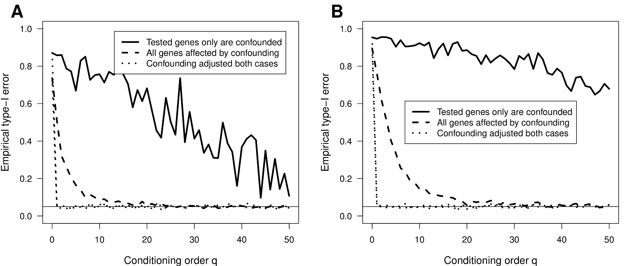
Figure 2: Explicit and implicit adjustment of confounding with higher-order conditional independence tests. Empirical type-I error rate for conditional independence tests from simulated data at a nominal level $\alpha=0.05$ (dotted horizontal line) as function of the conditioning order $q$. (A) Results on testing for an absent eQTL association; (B) results for an absent gene-gene association. Solid lines correspond to the model under which confounding affects only the tested genes while dashed lines correspond to a confounding effect on all genes. Dotted lines from both confounding models overlap because they correspond to the inclusion of the confounding effect in the conditioning subsets, thereby explicitly adjusting for it.

Figure 2 shows the empirical type-I error rate as function of the conditioning order $q$, where Figure 2A corresponds to the eQTL association and Figure 2B to the gene-gene association. This figure shows that, as expected, the explicit inclusion of the confounding factor in the conditioning subset $Q$ (dotted lines) adjusts the confounding effect immediately with $q>0$ in both situations, when either all genes are affected or only the tested ones. When the confounding effect is not included in $Q$ and affects only the tested genes (solid lines), it yields high type-I error rates that only decrease linearly with $n-q$, quantity on which statistical power depends. However, when confounding affects all genes (dashed lines) the type-I error rate has an exponential decay, and for $q>20$ the confounding effect is effectively adjusted in these data.

qp-Graph estimates of eQTL networks are enriched for cis-acting associations

Expression QTLs acting in cis have more direct mechanisms of regulation than those acting in trans (Rockman and Kruglyak 2006; Cheung and Spielman 2009). This hypothesis is supported by the observation that cis-acting eQTLs often explain a larger fraction of expression variance and show larger additive effects, than those acting in trans (Rockman and Kruglyak 2006; Petretto et al. 2006; Cheung and Spielman 2009). On the other hand, spurious eQTL associations tend to inflate the discovery of trans-acting eQTLs (Breitling et al. 2008). From this perspective, it makes sense to expect an enrichment of cis-eQTLs when indirect associations are effectively discarded (Kang et al. 2008; Listgarten et al. 2010).

We NRR values $\nu_{ij}^{q}$ on every pair $(i,j)$ of marker and gene from the yeast data set of $n=112$ segregants for different $q=\{25,50,75,100\}$ orders, restricting conditioning subsets to be formed by genes only. The resulting estimates $\hat{\nu}_{ij}^{q_{k}},q_{k}\in q$, were averaged, $\hat{\nu}_{ij}^{\bar{q}}=\frac{1}{|q|}\sum_{q_{k}}\hat{\nu}_{ij}^{q_{k}}$, to account for the uncertainty in the choice of the conditioning order $q$ (Castelo and Roverato 2009).

We ranked marker-gene pairs $(i,j)$ by average NRR values $\hat{\nu}_{ij}^{\bar{q}}$ and made a comparison against the ranking by $p$-value of the (exact) LRT for marginal independence (i.e., where $q=0$) to directly assess the added value of higher-order conditioning under the same type of statistical test. We considered conservative and liberal cutoff values $\epsilon=\{0.1,0.5\}$ on the average NRR $\hat{\nu}_{ij}^{\bar{q}}$ and obtained two different qp-graph estimates of the underlying eQTL network, denoted by $\hat{G}_{\epsilon}^{(\bar{q})}=(V,E_{\epsilon}^{(\bar{q})})$, each of them having $|E_{0.1}^{(\bar{q})}|=3,553$ and $|E_{0.5}^{(\bar{q})}|=55,562$ eQTL edges.

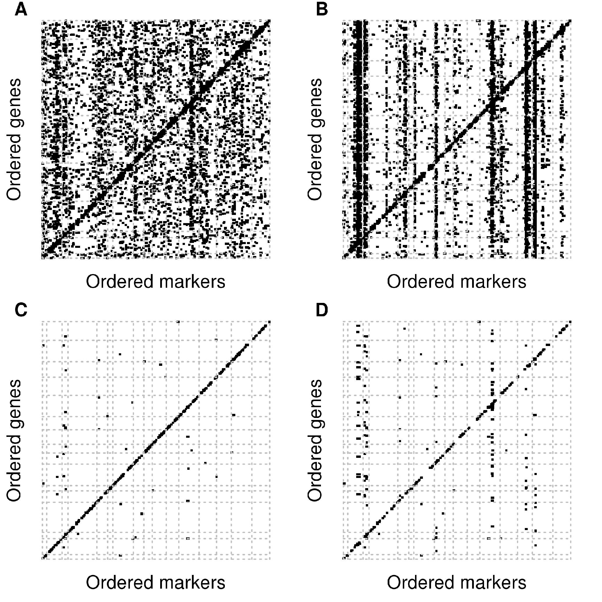
Figure 3: Enrichment of cis-acting eQTL associations. Dot plots of eQTL associations in yeast, where the $x$-axis and $y$-axis represent positions along the genome of markers and genes, respectively. Diagonal bands arise from cis-eQTLs while vertical ones from trans-eQTLs. Each row of two plots shows the top-$k$ eQTLs with largest strength in terms of non-rejection rates (A and C) and $p$-values for the null hypothesis of marginal independence (B and D), where $k$ is the number of eQTLs meeting a liberal (A) and conservative (C) cutoff on the non-rejection rate. Hence, plots in each row contain the same number of eQTLs.

We then selected the top-$k$ number of marker-gene pairs $(i,j)$ with lowest $p$-value in the marginal independence test, where $k=\{|E_{\epsilon}^{(\bar{q})}|\}$, which led to two other estimates of the eQTL network, denoted by $\hat{G}_{\epsilon}^{(0)}$. Note that both, $\hat{G}_{\epsilon}^{(\bar{q})}$ and $\hat{G}_{\epsilon}^{(0)}$, have the same number of edges, in this case, pairs $(i,j)$ of eQTL associations between a marker and a gene, thereby enabling a direct comparison of the fraction of cis- and trans-acting selected eQTL associations.

Table 1: Enrichment of cis-eQTL associations. Number of cis-eQTL associations in yeast found by the method introduced in this article (qpgraph) and by a marginal test of independence. Different columns correspond to different cutoffs (conservative, liberal) employed by qpgraph to select eQTLs, and different distances (500bp and 10Kb) to the gene TSS.

	Conservative cutoff (3,553 eQTLs)		Liberal cutoff (55,562 eQTLs)
Method	cis dist. 500bp	cis dist. 10Kb	cis dist. 500bp	cis dist. 10Kb
qpgraph	104	1,469	369	5,878
marginal	56	784	225	3,390
Enrichment	85%	87%	64%	73%

In Figure 3 we can see dot plots of the eQTL associations present in qp-graphs $\hat{G}_{\epsilon}^{(\bar{q})}$ (Figure 3, A and C), and those present in $\hat{G}_{\epsilon}^{(0)}$ using the marginal approach (Figure 3, B and D). Given the same number of eQTL associations, Figure 3 shows that qp-graph estimates of the underlying eQTL network have a higher number of cis-acting eQTLs than the marginal test, with an enrichment between 64% and 73% using the liberal cutoff, which increases to 85% and 87% using the conservative cutoff (see Table 1). Note that with the marginal approach more vertical bands of trans-acting associations remained present among the strongest selected eQTLs (Figure 3D), than with the qp-graph estimate (Figure 3C). We interpret this observation as evidence of the propagation of additive effects due to strong gene-gene correlations either present in the underlying eQTL network or created by confounding effects, and possibly aggravated by selection bias, as previously shown in Figure 1.

Performance comparison against another method

We compared the performance of the methodology introduced in this paper with a recent approach for causal inference among pairs of phenotypes (Chaibub Neto et al. 2013). This approach, called causal model selection tests (CMSTs), is implemented in the R/CRAN package qtlhot and can be used in 3 different ways (parametric, non-parametric and joint parametric), with two different penalized log-likelihood functions (AIC and BIC); see Chaibub Neto et al. (2013, pg. 1005) for details.

We ran the CMST analysis on the yeast data analyzed in this paper following the procedure described in (Chaibub Neto et al. 2013, pg. 1008-1010), which assessed performance using differential expression relationships obtained from a database of 247 knock-out (KO) experiments in yeast (Hughes et al. 2000; Zhu et al. 2008). To enable the comparison we used the raw CMST $p$-value of the so-called “$M_{3}$ independent model” (see Chaibub Neto et al. 2013, Figure 1) to build a ranking of 30,192 potential regulatory relationships, where each pair of genes had a common eQTL. We compared it against a corresponding ranking of NRR values estimated from the same data. Among these predicted associations 1,634 formed part of the database of 247 KO-experiments and using them as a bronze standard, we compared the two rankings by means of precision-recall curves. These are shown in Figure 4A and show nearly identical performance among all compared methods.

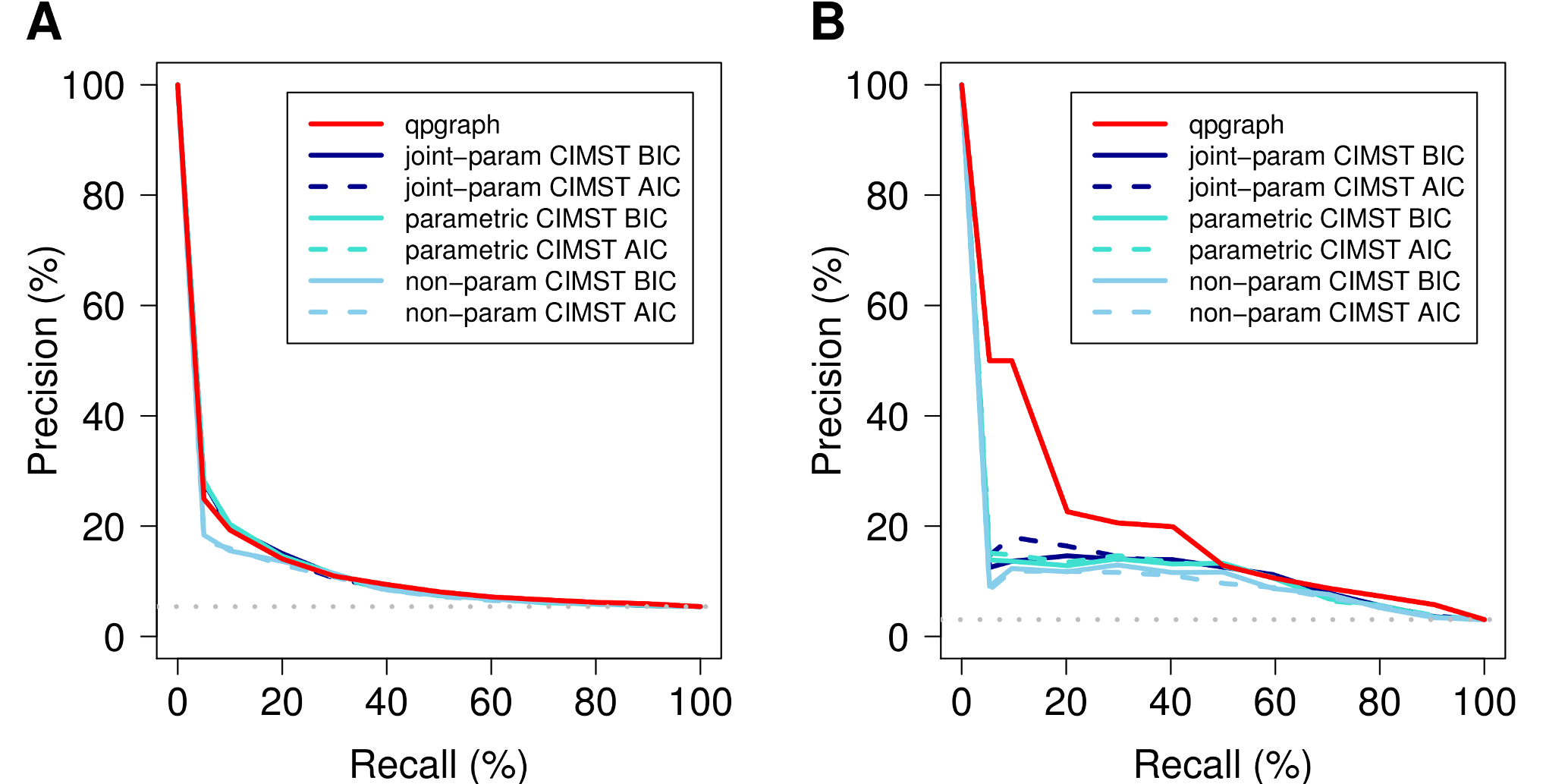
Figure 4: Comparison of qpgraph with qtlhot/CMST. Precision-recall curves calculated from predicted regulatory relationships inferred from a yeast cross data set using the approach introduced in this paper (qpgraph) and 6 different configurations of the qtlhot/CMST method. (A) Predictions are compared against a bronze standard formed by relationships formed by knocked-out genes and their putative targets derived from differential expression (Hughes et al. 2000; Zhu et al. 2008). (B) This bronze standard is further restricted to relationships also present in the Yeastract database (Teixeira et al. 2014) of curated transcriptional regulatory associations. The horizontal gray dotted line indicates the baseline precision attained by a random predictor.

Since a KO-gene may produce a cascade of expression changes, many of the 1,634 relationships in the bronze standard may actually be indirect, which would explain the similar performance using either lower (CMST) or higher (qpgraph) conditioning. We attempted to build a bronze standard of more direct regulatory relationships by first restricting the initial set of 30,192 possible associations to 3,074 that involved at least one transcription factor gene. Among these, we found 94 that were present in the database of KO experiments and in the Yeastract database of curated transcriptional regulatory relationships (Teixeira et al. 2014) and considered them as new bronze standard for comparison. The resulting precision-recall curves are shown in Figure 4B and reveal that NRR values estimated with qpgraph have larger discriminative power than CMSTs to identify direct regulatory interactions. Concretely, the area under the curve (AUC) for qpgraph is between 49% and 80% larger than the AUC of the different versions of CMSTs.

The genetic control of a gene-expression network in a yeast cross

We performed all pairwise exact tests of marginal independence on every marker-gene and gene-gene pair and corrected the resulting $p$-values by FDR to select those associations with FDR $<1\%$. The resulting graph, denoted by $\hat{G}^{(0)}$, had 92,710 eQTL and 2,203,119 gene-gene associations. The graph $\hat{G}^{(0)}$ constitutes a first estimate of the underlying eQTL network and it could be also obtained by the classical approach in QTL analysis of permuting phenotypes to test for the global null hypothesis of no QTL anywhere in the genome. Obviously, because the associations have been selected only using the margin of the data formed by one marker and one gene, or two genes, many of them will be indirect or spurious. To remove those associations we used the previously calculated average NRR values $\nu_{ij}^{(\bar{q})}$ and selected a conservative cutoff of $\epsilon=0.1$, so that a present association requires at least 90% of the conditional independence tests to be rejected. This resulted in an estimate $\hat{G}_{0.1}^{(\bar{q})}\subseteq\hat{G}^{(0)}$ formed by 3,498 eQTL and 1,799 gene-gene associations. Note that while the estimation of $\hat{G}^{(0)}$ requires some treatment of multiple testing, the NRR avoids this problem by actually exploiting the fact that is performing many tests to inform, by means of a Bernoulli variable, how close or far two genes, or a marker and a gene, are located in the network.

The genetic connected components of the eQTL network involved 450 genes and 3,498 eQTLs on 1,493 different loci, with a median of 6 eQTLs per gene. A substantial percentage of genes (27%) had $>10$ eQTLs on their own chromosome. Since eQTLs in $\hat{G}_{0.1}^{(\bar{q})}$ were independently mapped from each other, a fraction of those targeting a common gene may be tagging the same causal variant. We removed redundant eQTLs by the following forward selection procedure. For each gene, we ordered its linked eQTLs by increasing NRR values $\nu_{ij}^{(\bar{q})}$ and proceeded over the ranked eQTLs to test the conditional independence of the gene and the eQTL, given the eQTLs occurring before in the ranking using again the exact test described in the Methods section. An eQTL association was retained if the test was rejected at $p<0.05$ and the selection procedure stopped whenever $p>0.05$ to continue on the next gene.

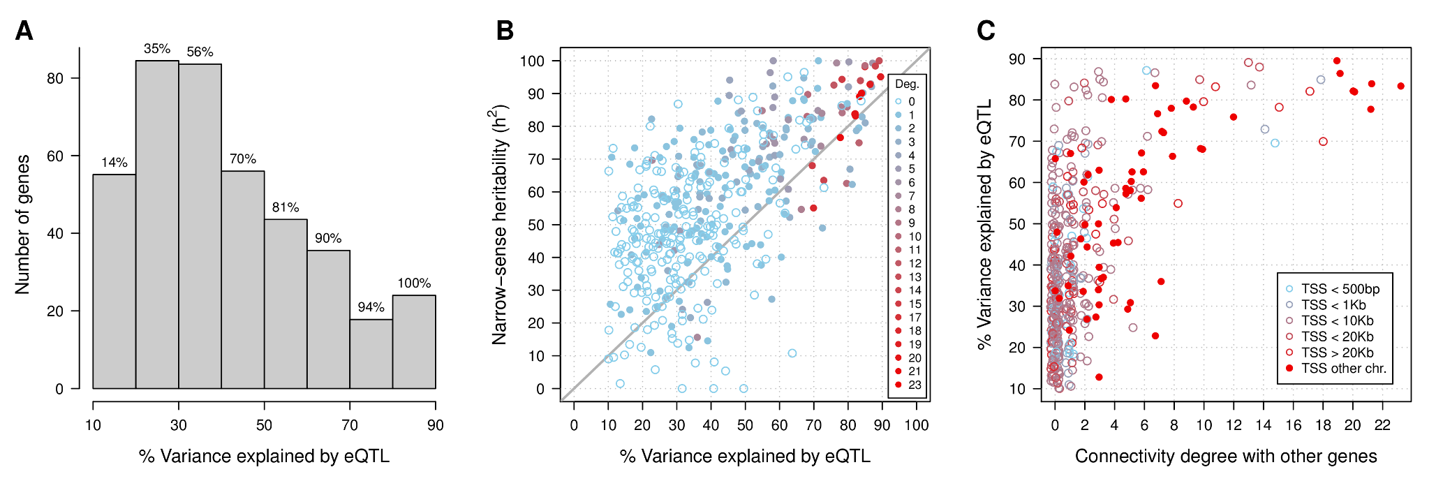
Figure 5: Variance explained in the eQTL network. (A) Distribution of the percentage of gene expression variance explained by eQTLs. The cumulative percentage of genes is reported on top of each bar. (B) Scatter plot of the narrow-sense heritability $h^{2}$ as function of the percentage of variance explained by eQTLs. The diagonal line is drawn at values where this percentage equals $h^{2}$, and it is only shown as a visual guide. Open circles correspond to genes with exclusively eQTL associations while solid ones indicate also the presence of at least one association with other gene. The legend contains the color key for the degree of association in the network. (C) Percentage of variance explained by eQTLs as function of the degree of association with other genes in the network. The legend specifies the color key for the average distance from the transcription start site (TSS) of the gene to its eQTLs.

The genetic connected components were substantially pruned and the vast majority of genes (402/450) were left with just one eQTL, 46 genes with two, and only two had 3 eQTLs. This final eQTL network comprised 500 eQTLs and 1,391 genes, the vast majority of them (941) forming gene-gene associations without any eQTL.

Hub genes have trans-acting eQTLs with large genetic effects: For each of the 450 genes having at least one eQTL, we calculated the percentage of variance explained by eQTLs using Eq. (31). The distribution of resulting values is shown in Fig. 5A. About 70% of the genes had eQTLs explaining 50% or less of their expression variability, and only in about 10% of them their eQTLs explained $>70$%.

Using a method based on linear mixed modeling and exploiting the relatedness matrix built from all pairs of segregants (Lee et al. 2011; Bloom et al. 2013) we estimated the narrow-sense heritability $h^{2}$ for these 450 genes and compared it against the percentage of variance explained by the eQTLs (Fig. 5B). Setting the percentage explained to the expected maximum $h^{2}$ when the former was larger, the fraction of missing heritability ranges from 0% to 62%. This figure also shows that the connectivity degree to other genes correlates positively with both, $h^{2}$ and percentage of variance explained. In fact, as Figure 5C shows, there are 24 genes connected to 9 or more other genes, for which all their eQTLs explain 68% or more of their expression variability. Interestingly, this figure also reveals that half of them have a trans-acting eQTL located in a different chromosome. In fact, these particular trans-eQTLs map all of them to chromosomes II and III (Table 2). Concretely, the eQTL of gene SCW11 is located in position 553,857 of chromosome II, 2.6Kb away from the AMN1 gene. This gene carries a loss-of-function mutation in the BY strain (Yvert et al. 2003) affecting the expression of daughter-cell-specific genes. The eQTLs in chromosome III map to the MAT and LEU2 loci, the latter being one of the engineered deletions in the BY strain.

Table 2: Hub genes connected to 9 or more other genes in the eQTL network. The column “Pathway” specifies the primary pathway or molecular process in which the gene is involved, where (*) indicates that the gene has unknown function and its pathway has been predicted using the eQTL network. The column “Location” reports the chromosomes where the gene’s eQTLs are located. When both gene and eQTLs are in the same chromosome, the column distance reports the average distance between them. Columns $h^{2}$ and $\eta^{2}$ report, respectively, the narrow-sense heritability and the fraction of variance explained by the eQTL. The column “Deg.” (degree) gives the number of associated genes in the network.

Gene	Chr	Pathway	Location	Distance	$h^{2}$	$\eta^{2}$	Deg.
STE2	VI	Mating reg.	III	NA	0.89	0.83	23
YKL177W	XI	Mating reg.	III	NA	0.77	0.78	21
STE3	XI	Mating reg.	III	NA	0.90	0.84	21
BAR1	IX	Mating reg.	III	NA	0.83	0.82	20
MF(ALPHA)1	XVI	Mating reg.	III	NA	0.84	0.82	20
STE6	XI	Mating reg.	III	NA	0.95	0.90	19
AFB1	XII	Mating reg.	III	NA	0.93	0.86	19
HMLALPHA2	III	Mating reg.	III	188156	0.55	0.70	18
MATALPHA1	III	Mating reg.	III	732	0.98	0.85	18
HMLALPHA1	III	Mating reg.	III	187892	0.84	0.82	17
YCL065W	III	Mating reg. (*)	III	187423	0.94	0.78	15
YCR041W	III	Mating reg. (*)	III	263	0.68	0.70	15
MATALPHA2	III	Mating reg.	III	996	0.63	0.73	14
ASP3-3	XII	Nitr. starvation	XII	14538	0.98	0.88	14
ASP3-1	XII	Nitr. starvation	XII	10806	1.00	0.89	13
ASP3-2	XII	Nitr. starvation	XII	5046	0.94	0.84	13
LEU1	VII	Leu biosynthesis	III	NA	0.93	0.76	12
YCR097W-A	III	Mating reg. (*)	III	105944	0.75	0.83	11
HMRA1	III	Mating reg.	III	88278	0.63	0.80	10
BAT1	VIII	Leu biosynthesis	III	NA	0.83	0.68	10
OAC1	XI	Leu biosynthesis	III	NA	0.90	0.68	10
ASP3-4	XII	Nitr. starvation	XII	18190	0.98	0.85	10
SCW11	VII	Daugh. cell sep.	II	NA	0.86	0.80	9
MFA2	XIV	Mating reg.	III	NA	0.84	0.78	9

Genes YCL065W, YCR041W and YCR097W-A in Table 2 have currently unknown function. However, a Gene Ontology (GO) enrichment analysis on each subset of genes connected to them in the eQTL network showed that they are potentially involved in mating-specific regulatory processes (Holm’s FWER $<0.05$).

Therefore, these highly-connected genes, shown in Table 2, are involved in regulatory processes related to mating-specific expression, reacting upon nitrogen starvation, participation in the leucine biosynthesis pathway and daughter cell separation. These are fundamental pathways for yeast growth and render these results consistent with previous evidence from yeast genetic interaction networks derived from double-mutant screens (Costanzo et al. 2010), where highly-connected genes were involved in primary cellular functions (Baryshnikova et al. 2013).

Differential genetic control of gene expression across chromosomes: We also investigated how genetic variation affects gene expression differently across the yeast chromosomes. For this purpose, we produced hive plots (Krzywinski et al. 2012) shown in Figure 6, using the R/CRAN package HiveR (Hanson 2014). A first observation is that eQTLs occurring within the same chromosome (edges between the markers axis and genes axis of the same chromosome) mostly lead to concentric edges, pointing to cis-regulatory mechanisms acting at different distances. A remarkable exception is chromosome III where many of those edges cross through each other. This chromosome is also distinctive in that it has a lower density of cis-acting eQTLs than the rest of the genome.

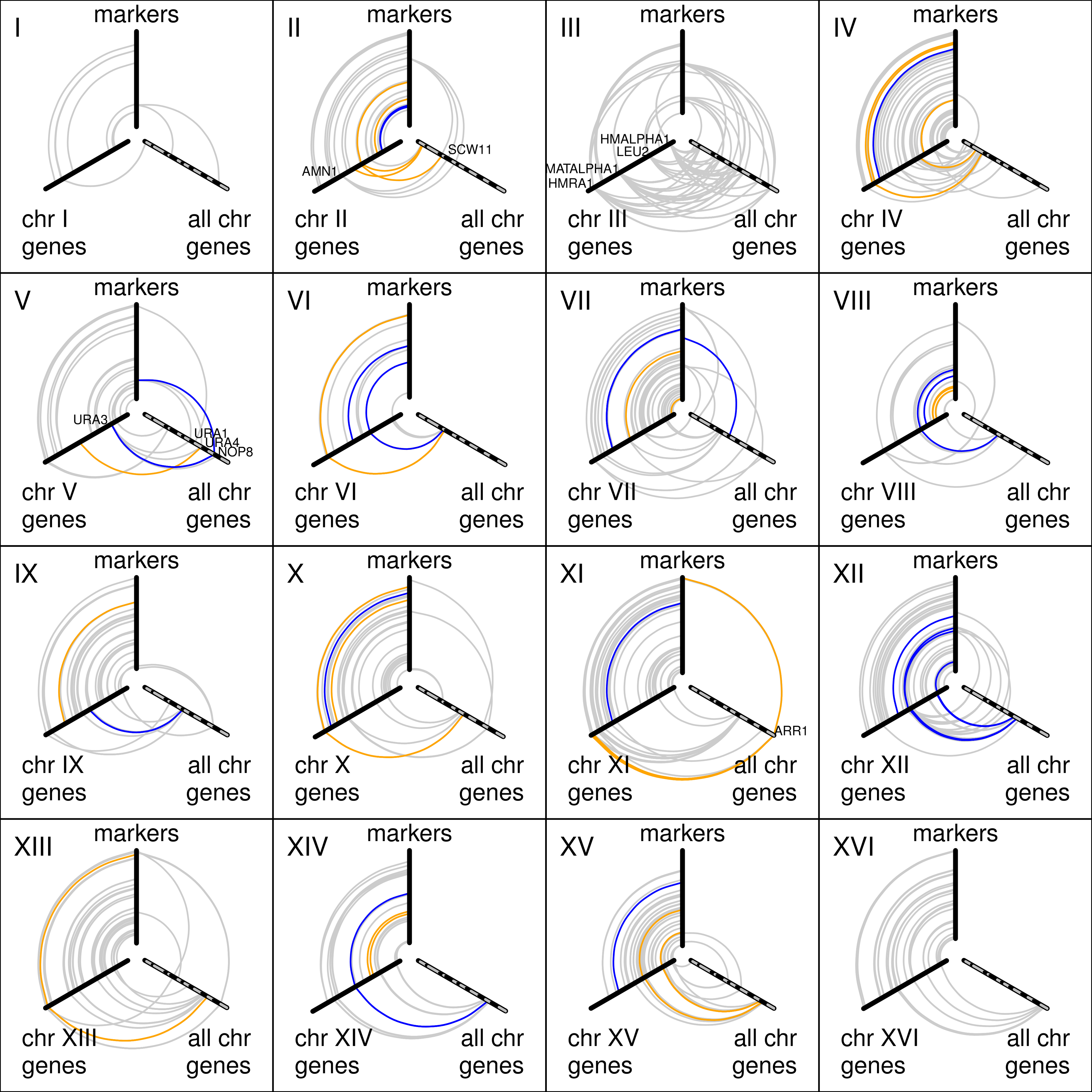
Figure 6: eQTL network of a yeast cross. Hive plots of an eQTL network estimated from a yeast cross, involving only connected components with at least one eQTL association. For each chromosome, the hive plot shows three axes, where markers and genes are ordered from the center according to their genomic location. Vertical and left axes represent the chromosome in the corresponding plot, while the right axis represents the entire yeast genome alternating black and gray along consecutive chromosomes. Edges between genes axes correspond to gene-gene associations. Edges where at least one of their endpoints corresponds to a transcription factor or RNA-binding coding gene, are highlighted in orange and blue, respectively.

Between 81Kb and 92Kb from the beginning of chromosome III there is a cis-acting eQTL on genes LEU2 and NFS1. This eQTL is also trans-associated with genes BAT1, OAC1, LEU1 and BAP2 located in different chromosomes and involved in the leucine biosynthesis pathway. According to the UCSC Genome Browser (http://genome.ucsc.edu) they all have upstream a binding site of LEU3, a major regulatory switch in this pathway. The engineered deletion of LEU2 affects LEU3 in a feedback loop and this would lead to expression changes in its targets (Chin et al. 2008).

Downstream, at about 200Kb of the beginning of chromosome III, we find the MAT locus whose genetic composition determines the mating type of yeast. This eQTL is cis-associated with the gene MATALPHA1 which is expressed in haploids of the alpha mating type and which has been previously reported as a candidate regulator of the rest of genes associated with this locus (Yvert et al. 2003; Curtis et al. 2013). This locus is trans-associated with two other genes in the same chromosome (HMLALPHA1, HMRA1) and to a set of genes distributed throughout the genome (STE2, STE3, STE6, AFB1, BAR1, MF(ALPHA)1, MFA2) which are all involved in the regulation of mating-type specific transcription.

In chromosome V, around the locus of URA3 we find a cis-acting eQTL which has a trans-acting effect on URA1 (chrom. XI) and URA4 (chrom. XII), the three of them taking part in the biosynthesis of pyrimidines (Yvert et al. 2003; Curtis et al. 2013). As it can be easily seen from Figure 6, and consistent with previous observations (Yvert et al. 2003), few of the eQTLs affect directly transcription factors, such as the ARR1 gene in chromosome XI, or RNA-binding proteins, such as NOP8 in chromosome V.

The edges between the genes axes, correspond to gene-gene associations from the corresponding chromosome to the rest of the genome and where at least one of the genes has an eQTL. This is a fraction (503) of a total of 1,799 gene-gene associations on the entire eQTL network, more directly affected by the genetic control of gene expression. We observed a systematic pattern of association between genes from the same chromosome (see, e.g., chrom. XVI). Replacing the axis displaying genes from all chromosomes by another gene axis again of the same chromosome (data not shown) reveals that a fraction of the gene-gene associations in which one of the genes has a cis-acting eQTL, occur between genes close to each other on the chromosome. It may be possible that inherited coexpression segregates due to linkage disequilibrium and/or that tandem gene duplication events render genes close to each other being coexpressed. Using the strategies introduced in this paper further, such as conditioning these associations on nearby genes, may help to elucidate what fraction of them are of genetic, molecular or evolutionary origin.

Discussion

Gene expression is a high-dimensional multivariate trait whose variability is the result of genetic, molecular and environmental perturbations, and often different kinds of confounding effects. Dissecting the components of this variability and being able to adjust for some of them is a major goal in every study using genetical genomics data. Here we have used a class of statistical models with a graphical interpretation, mixed GMMs, to approach this challenge from a multivariate perspective. Using simulations we have shown that genetic effects can propagate proportionally to the marginal correlation between the genes, and that this effect may be amplified under selection bias (Fig. 1), underscoring the need to adjust for indirect associations.

Using standard linear theory and basic principles from mixed GMMs, we have derived the parameters, in terms of a mixed GMM, for an exact likelihood-ratio test (LRT) on data from conditional Gaussian distributions that accommodate both linear and interaction effects between genetic variants and continuous gene-expression profiles. Higher-order conditioning on mixed data unlocks a number of strategies that one may follow to disentangle direct and indirect effects in genetical genomics experiments. We exploited it by using marginal distributions and $q$-order correlation graphs. We showed that this approach allows one to adjust for confounding effects (Fig. 2), increases our power to identify cis-acting eQTLs (Fig. 3) and direct regulatory relationships (Fig. 4), and helped comparing the genetic control of gene expression between chromosomes (Fig. 6) and throughout the gene network (Fig. 5). In particular, we could see that the degree of connections of each eQTL gene to other genes in the eQTL network correlated positively with both, narrow-sense heritability and fraction of variance explained by eQTLs (Fig. 5). An important fraction of large genetic effects were in fact due to trans-acting eQTLs from those genes with more connections. Using those connections we could predict potential pathways involving three such hub genes of unknown function. Genetical genomics data from large experimental crosses are becoming increasingly available to the community. We believe that mixed GMMs can play a crucial role in harnessing these data to explore linear and interacting eQTL associations of arbitrary order and advance our understanding of the genetic control of gene expression.

Literature Cited

- Baryshnikova et al. (2013) Baryshnikova, A., M. Costanzo, C. L. Myers, B. Andrews, and C. Boone, 2013 Genetic interaction networks: Toward an understanding of heritability. Annu Rev Genom Hum G 14: 111–133.
- Bing and Hoeschele (2005) Bing, N., and I. Hoeschele, 2005 Genetical genomics analysis of a yeast segregant population for transcription network inference. Genetics 170: 533–42.
- Bloom et al. (2013) Bloom, J. S., I. M. Ehrenreich, W. T. Loo, T.-L. V. Lite, and L. Kruglyak, 2013 Finding the sources of missing heritability in a yeast cross. Nature 494: 234–237.
- Breitling et al. (2008) Breitling, R., Y. Li, B. M. Tesson, J. Fu, C. Wu, et al., 2008 Genetical genomics: spotlight on QTL hotspots. PLoS Genet 4: e1000232.
- Brem and Kruglyak (2005) Brem, R. B., and L. Kruglyak, 2005 The landscape of genetic complexity across 5,700 gene expression traits in yeast. P Natl Acad Sci USA 102: 1572–7.
- Brem et al. (2002) Brem, R. B., G. Yvert, R. Clinton, and L. Kruglyak, 2002 Genetic dissection of transcriptional regulation in budding yeast. Science 296: 752–755.
- Broman and Sen (2009) Broman, K. W., and S. Sen, 2009 A guide to QTL mapping with R/qtl. Springer.
- Broman et al. (2003) Broman, K. W., H. Wu, S. Sen, and G. A. Churchill, 2003 R/qtl: QTL mapping in experimental crosses. Bioinformatics 19: 889–890.
- Castelo and Roverato (2006) Castelo, R., and A. Roverato, 2006 A robust procedure for Gaussian graphical model search from microarray data with p larger than n. J Mach Learn Res 7: 2621–50.
- Castelo and Roverato (2009) Castelo, R., and A. Roverato, 2009 Reverse engineering molecular regulatory networks from microarray data with qp-graphs. J Comput Biol 16: 213–227.
- Chaibub Neto et al. (2013) Chaibub Neto, E., A. T. Broman, M. P. Keller, A. D. Attie, B. Zhang, et al., 2013 Modeling causality for pairs of phenotypes in systems genetics. Genetics 193: 1003–1013.
- Chaibub Neto et al. (2008) Chaibub Neto, E., C. T. Ferrara, A. D. Attie, and B. S. Yandell, 2008 Inferring causal phenotype networks from segregating populations. Genetics 179: 1089–100.
- Chaibub Neto et al. (2010) Chaibub Neto, E., M. P. Keller, A. D. Attie, and B. S. Yandell, 2010 Causal graphical models in systems genetics: a unified framework for joint inference of causal network and genetic architecture for correlated phenotypes. Ann Appl Stat 4: 320–339.
- Chen et al. (2007) Chen, L. S., F. Emmert-Streib, and J. D. Storey, 2007 Harnessing naturally randomized transcription to infer regulatory relationships among genes. Genome Biol 8: R219.
- Cheung and Spielman (2009) Cheung, V. G., and R. S. Spielman, 2009 Genetics of human gene expression: mapping DNA variants that influence gene expression. Nat Rev Genet 10: 595–604.
- Chin et al. (2008) Chin, C.-S., V. Chubukov, E. R. Jolly, J. DeRisi, and H. Li, 2008 Dynamics and design principles of a basic regulatory architecture controlling metabolic pathways. PLoS Biol 6: e146.
- Chun and Keleş (2009) Chun, H., and S. Keleş, 2009 Expression quantitative trait loci mapping with multivariate sparse partial least squares regression. Genetics 182: 79–90.
- Costanzo et al. (2010) Costanzo, M., A. Baryshnikova, J. Bellay, Y. Kim, E. D. Spear, et al., 2010 The genetic landscape of a cell. Science 327: 425–431.
- Curtis et al. (2013) Curtis, R. E., S. Kim, J. L. Woolford Jr, W. Xu, and E. P. Xing, 2013 Structured association analysis leads to insight into Saccharomyces cerevisiae gene regulation by finding multiple contributing eQTL hotspots associated with functional gene modules. BMC Genomics 14: 1–17.
- Didelez and Edwards (2004) Didelez, V., and D. Edwards, 2004 Collapsibility of graphical cg-regression models. Scand J Stat 31: 535–551.
- Edwards (2000) Edwards, D., 2000 Introduction to graphical modelling. Springer.
- Edwards et al. (2010) Edwards, D., G. C. G. de Abreu, and R. Labouriau, 2010 Selecting high-dimensional mixed graphical models using minimal aic or bic forests. BMC Bioinformatics 11: 18.
- Grone et al. (1984) Grone, R., C. Johnson, E. Sá, and H. Wolkowicz, 1984 Positive definite completions of partial Hermitian matrices. Linear Algebra Appl 58: 109–124.
- Hanson (2014) Hanson, B. A., 2014 HiveR: 2D and 3D Hive plots for R. R/CRAN pkg. ver. 0.2-27.
- Hastie et al. (2009) Hastie, T., R. Tibshirani, and J. Friedman, 2009 The elements of statistical learning. Springer.
- Hughes et al. (2000) Hughes, T. R., M. J. Marton, A. R. Jones, C. J. Roberts, R. Stoughton, et al., 2000 Functional discovery via a compendium of expression profiles. Cell 102: 109–126.
- Jansen and Nap (2001) Jansen, R. C., and J.-P. Nap, 2001 Genetical genomics: the added value from segregation. Trends Genet 17: 388–390.
- Kalisch and Bühlmann (2007) Kalisch, M., and P. Bühlmann, 2007 Estimating high-dimensional directed acyclic graphs with the pc-algorithm. J Mach Learn Res 8: 613–636.
- Kang et al. (2010) Kang, E. Y., C. Ye, I. Shpitser, and E. Eskin, 2010 Detecting the presence and absence of causal relationships between expression of yeast genes with very few samples. J Comput Biol 17: 533–46.
- Kang et al. (2008) Kang, H. M., C. Ye, and E. Eskin, 2008 Accurate discovery of expression quantitative trait loci under confounding from spurious and genuine regulatory hotspots. Genetics 180: 1909–25.
- Kendziorski et al. (2006) Kendziorski, C., M. Chen, M. Yuan, H. Lan, and A. Attie, 2006 Statistical methods for expression quantitative trait loci (eQTL) mapping. Biometrics 62: 19–27.
- Kim and Xing (2009) Kim, S., and E. P. Xing, 2009 Statistical estimation of correlated genome associations to a quantitative trait network. PLoS Genet 5: e1000587.
- Krzywinski et al. (2012) Krzywinski, M., I. Birol, S. J. Jones, and M. A. Marra, 2012 Hive plots–rational approach to visualizing networks. Brief Bioinform 13: 627–644.
- Lauritzen (1996) Lauritzen, S., 1996 Graphical Models. Oxford University Press.
- Lauritzen and Wermuth (1989) Lauritzen, S., and N. Wermuth, 1989 Graphical models for associations between variables, some of which are qualitative and some quantitative. Ann Stat 17: 31–57.
- Lee et al. (2011) Lee, S. H., N. R. Wray, M. E. Goddard, and P. M. Visscher, 2011 Estimating missing heritability for disease from genome-wide association studies. Am J Hum Genet 88: 294–305.
- Leek et al. (2010) Leek, J. T., R. B. Scharpf, H. C. Bravo, D. Simcha, B. Langmead, et al., 2010 Tackling the widespread and critical impact of batch effects in high-throughput data. Nat Rev Genet 11: 733–739.
- Leek and Storey (2007) Leek, J. T., and J. D. Storey, 2007 Capturing heterogeneity in gene expression studies by surrogate variable analysis. PLoS Genet 3: e161.
- Li et al. (2002) Li, Q., K. R. Peterson, X. Fang, and G. Stamatoyannopoulos, 2002 Locus control regions. Blood 100: 3077–3086.
- Listgarten et al. (2010) Listgarten, J., C. Kadie, and D. Heckerman, 2010 Correction for hidden confounders in the genetic analysis of gene expression. P Natl Acad Sci USA 107: 16465–16470.
- Liu et al. (2008) Liu, B., A. de la Fuente, and I. Hoeschele, 2008 Gene network inference via structural equation modeling in genetical genomics experiments. Genetics 178: 1763–76.
- Michaelson et al. (2010) Michaelson, J. J., R. Alberts, K. Schughart, and A. Beyer, 2010 Data-driven assessment of eQTL mapping methods. BMC genomics 11: 502.
- Montgomery et al. (2010) Montgomery, S. B., M. Sammeth, M. Gutierrez-Arcelus, R. P. Lach, C. Ingle, et al., 2010 Transcriptome genetics using second generation sequencing in a caucasian population. Nature 464: 773–777.
- Parts et al. (2011) Parts, L., O. Stegle, J. Winn, and R. Durbin, 2011 Joint genetic analysis of gene expression data with inferred cellular phenotypes. PLoS Genet 7: e1001276.
- Petretto et al. (2006) Petretto, E., J. Mangion, N. J. Dickens, S. A. Cook, M. K. Kumaran, et al., 2006 Heritability and tissue specificity of expression quantitative trait loci. PLoS Genet 2: e172.
- Rao (1973) Rao, C., 1973 Linear Statistical Inference and Its Applications. John Wiley & Sons.
- Ritchie et al. (2007) Ritchie, M. E., J. Silver, A. Oshlack, M. Holmes, D. Diyagama, et al., 2007 A comparison of background correction methods for two-colour microarrays. Bioinformatics 23: 2700–2707.
- Rockman (2008) Rockman, M. V., 2008 Reverse engineering the genotype–phenotype map with natural genetic variation. Nature 456: 738–744.
- Rockman and Kruglyak (2006) Rockman, M. V., and L. Kruglyak, 2006 Genetics of global gene expression. Nat Rev Genet 7: 862–872.
- Roverato (2002) Roverato, A., 2002 Hyper inverse Wishart distribution for non-decomposable graphs and its application to Bayesian inference for Gaussian graphical models. Scand J Stat 29: 391–411.
- Schadt et al. (2003) Schadt, E. E., S. A. Monks, T. A. Drake, A. J. Lusis, N. Che, et al., 2003 Genetics of gene expression surveyed in maize, mouse and man. Nature 422: 297–302.
- Seber (2007) Seber, G., 2007 A matrix handbook for statisticians. Wiley-Interscience.
- Smyth and Speed (2003) Smyth, G. K., and T. Speed, 2003 Normalization of cDNA microarray data. Methods 31: 265–273.
- Stegle et al. (2010) Stegle, O., L. Parts, R. Durbin, and J. Winn, 2010 A Bayesian framework to account for complex non-genetic factors in gene expression levels greatly increases power in eQTL studies. PLoS Comp Biol 6: e1000770.
- Teixeira et al. (2014) Teixeira, M. C., P. T. Monteiro, J. F. Guerreiro, J. P. Gonçalves, N. P. Mira, et al., 2014 The YEASTRACT database: an upgraded information system for the analysis of gene and genomic transcription regulation in Saccharomyces cerevisiae. Nucleic Acids Res 42: D161–D166.
- Tesson and Jansen (2009) Tesson, B. M., and R. C. Jansen, 2009 eQTL analysis in mice and rats. In Cardiovascular Genomics, volume 573 of Methods in Molecular Biology. Springer, 285–309.
- Westra et al. (2013) Westra, H.-J., M. J. Peters, T. Esko, H. Yaghootkar, C. Schurmann, et al., 2013 Systematic identification of trans eQTLs as putative drivers of known disease associations. Nat Genet 45: 1238–1243.
- Yvert et al. (2003) Yvert, G., R. B. Brem, J. Whittle, J. M. Akey, E. Foss, et al., 2003 Trans-acting regulatory variation in Saccharomyces cerevisiae and the role of transcription factors. Nat Genet 35: 57–64.
- Zhu et al. (2004) Zhu, J., P. Y. Lum, J. Lamb, D. GuhaThakurta, S. W. Edwards, et al., 2004 An integrative genomics approach to the reconstruction of gene networks in segregating populations. Cytogenet Genome Res 105: 363–74.
- Zhu et al. (2008) Zhu, J., B. Zhang, E. N. Smith, B. Drees, R. B. Brem, et al., 2008 Integrating large-scale functional genomic data to dissect the complexity of yeast regulatory networks. Nat Genet 40: 854–861.