Application of the Ring Theory in the Segmentation
of Digital Images

Abstract

Ring theory is one of the branches of the abstract algebra that has been broadly used in images. However, ring theory has not been very related with image segmentation. In this paper, we propose a new index of similarity among images using $\mathbb{Z}_{n}$ rings and the entropy function. This new index was applied as a new stopping criterion to the Mean Shift Iterative Algorithm with the goal to reach a better segmentation. An analysis on the peformance of the algorithm with this new stopping criterion is carried out. The obtained results proved that the new index is a suitable tool to compare images.

1 Introduction

Many techniques and algorithms have been proposed for digital image segmentation. Traditional segmentation such as thresholding, histograms or other conventional operations are rigid methods. Automation of these classical approximations is difficult due to the complexity in shape and variability within each individual object in the image.

The mean shift is a non-parametric procedure that has demostrated to be an extremely versatile tool for feature analysis. It can provide reliable solutions for many computer vision tasks [2]. Mean shift method was proposed in 1975 by Fukunaga and Hostetler [5]. It was largely forgotten until Cheng’s paper retook interest on it [1]. Segmentation by means of the Mean Shift Method carries out as a first step a smoothing filter before segmentation is performed [2, 3].

Entropy is an essential function in information theory and this has had a special uses for images data, e.g., restoring images, detecting contours, segmenting images and many other applications [12, 15]. However, in the field of images the range of properties of this function could be increased if the images are defined in $\mathbb{Z}_{n}$ rings. The inclusion of the ring theory to the spatial analysis is achieved considering images as a matrix in which the elements belong to the cyclic ring $\mathbb{Z}_{n}$. From this point of view, the images presents cyclical properties associated to gray level values.

Ring Theory has been well-used in cryptography and many others computer vision tasks [18]. The inclusion of ring theory to the spatial analysis of digital images, it is achieved considering the image like a matrix in which the elements belong to finite cyclic ring $\mathbb{Z}_{n}$. The ring theory for the Mean Shift Iterative Algorithm was employed by defining images in a ring $\mathbb{Z}_{n}$. A good performance of this algorithm was achieved. Therefore, the use of the ring theory could be a good structure when one desires to compare images, due to that the digital images present cyclical properties associated with the pixel values. This property will allow to increase or to diminish the difference among pixels values, and will make possible to find the edges in the analyzed images.

In this paper, a new similarity index among images is defined, and some interesting properties based on this index are proposed. We compare also the instability of the iterative mean shift algorithm ($\mathit{MSHi}$) by using this new stopping criterion with regard to the stopping criterion used in [8, 9, 10, 11]. Furthermore, we make an extension of [7], and we expand the theoretical aspects by studying in depth the cyclical properties of rings applied to images. For this purpose, and in order to mark the difference of this paper with regard to [7], some issues are pointed out below:

• Revision of the mean shift theory.

• Important elements of the ring $G_{k\times m}(\mathbb{Z}_{n})(+,\cdot)$ are given: neutral, unitary, and inverse. In particular, the inverse element was used so much to the theoretical proofs as well as practical aspects.

• Explanation of strong equivalent images by using histograms.

• Definition of equivalence classes.

• Quotient space. Definition and existence.

• Natural Entropy Distance (NED) definition.

• Configuration of the algorithm $\mathit{MSHi}$ with the NED distance.

The remainder of the paper is organized as follows. In Section 2, the more significant theoretical aspects of the mean shift and entropy are given. Section 3 describes the similarity index, its consecuences for entropy function and the significance of the cyclic ring $\mathbb{Z}_{n}$ for images. Also, it is defined the quotient space of strongly equivalent images and some properties of entropy are proved. The experimental results, comparisons and discussion are presented in Section 4. Finally, in Section 5 the conclusions are given.

2 Theoretical Aspects

2.1 Mean Shift

One of the most popular nonparametric density estimators is kernel density estimation. Mathematically, the general multivariate kernel density estimate at the point $x$, is defined by:

$$f(x)=\frac{1}{nh^{d}}\sum\limits_{i=1}^{n}K\left(\frac{x-x_{i}}{h}\right).$$ (1)

where $n$ data points $x_{i},\ i=1,\ldots,n$ represent a population with some unknown density function $f(x)$.

In the case of images:

$$K_{H}(x)=|H|^{-1/2}K\left(H^{-1/2}x\right)$$ (2)

where $K(z)$ is the $d-variate$ kernel function with compact support satisfying the regularity constraints as described in [16], and $H$ is a symmetric positive definite bandwidth matrix.

For image segmentation, the feature space is composed of two independent domains: the $spatial/lattice$ domain and the $range/color$ domain. We map a pixel to a multidimensional feature point which includes the $p$ dimensional spatial lattice ($p=2$ for image) and $q$ dimensional color ($q=1$ for gray scale images and $q=3$ for color image and $q>3$ for multispectral image). Due to the different natures of the domains, the kernel is usually broken into the product of two different radially symmetric kernels (subscript $s$ is refer to the spatial domain, and $r$ to the color range):

$$K_{h_{s},h_{r}}(x)=\frac{c}{(h_{s})^{p}(h_{r})^{q}}k_{s}\left(\left\lVert\frac{x}{h_{s}}\right\rVert^{2}\right)k_{r}\left(\left\lVert\frac{x}{h_{r}}\right\rVert^{2}\right)$$ (3)

where $x$ is a pixel, $k_{s}$ and $k_{r}$ are the profiles used in the two respective domains, $h_{s}$ and $h_{r}$ are employed bandwidths in $spatial-range$ domains and $c$ is the normalization constant. Using the equation (3), the kernel density estimator is:

$$\hat{f}(x)=\frac{c}{n(h_{s})^{p}(h_{r})^{q}}\sum_{i=1}^{n}k_{s}\left(\left\lVert\frac{x-x_{i}}{h_{s}}\right\rVert^{2}\right)k_{r}\left(\left\lVert\frac{x-x_{i}}{h_{r}}\right\rVert^{2}\right).$$ (4)

As was shown in (3) and (4), there are two main parameters that have to be defined by the user: the spatial bandwidth $h_{s}$ and the range bandwidth $h_{r}$.

The Epanechnikov function is chosen as the kernel function in this work, this function is defined as:

$$K_{E}(x)=\left\{\begin{array}[]{ll}\frac{1}{2}c^{-1}_{d}(d+2)\left(1-\left\|x\right\|^{2}\right),&\mbox{if}\ \left\|x\right\|<1\\ &\\ 0,&\mbox{otherwise}.\\ \end{array}\right.$$ (8)

The gradient of function $f(x)$ is formulated as

$$\widehat{\nabla}f(x)=\nabla\widehat{f(x)}=\frac{1}{nh^{d}}\sum\limits_{i=1}^{n}\widehat{K}\left(\frac{x-x_{i}}{h}\right),$$ (9)

$$\widehat{\nabla}f_{E}(x) =\frac{1}{n(h^{d}c_{d})}\frac{d+2}{h^{2}}\sum\limits_{x_{i}\in S_{h}(x)}(x_{i}-x)$$

$$=\frac{n_{x}}{n(h^{d}c_{d})}\frac{d+2}{h^{2}}\frac{1}{n_{x}}\sum\limits_{x_{i}\in S_{h}(x)}(x_{i}-x),$$ (10)

where region $S_{h}(x)$ is a hypersphere of radius $h$ having volume $h^{d}c_{d}$, centred at $x$, and containing $n_{x}$ data points; that is, the uniform kernel. By simplicity, in this paper, we only approach the case $d=1$ corresponding to gray level images, but could be extended in the same way to color ($d=3$) and multispectral ($d>3$) images. In addition, the last factor in expression (2.1) is called the sample mean shift

$$M_{h,U}(x)=\underbrace{\frac{1}{n_{x}}\sum\limits_{x_{i}\in S_{h}(x)}(x_{i}-x)}_{\text{\large mean of shift values}}=\underbrace{\left(\frac{1}{n_{x}}\sum\limits_{x_{i}\in S_{h}(x)}x_{i}\right)-x}_{\text{\large mean shift}}$$ (11)

The quantity $\displaystyle\frac{n_{x}}{n(h^{d}c_{d})}$ is the kernel density estimate $\widehat{f_{U}}(x)$ (where $U$ means the uniform kernel) computed with the hyper sphere $S_{h}(x)$, and thus we can write the expression (2.1) as:

$$\widehat{\nabla}f_{E}(x)=\widehat{f_{U}}(x)\frac{d+2}{h^{2}}M_{h,U}(x)$$ (12)

which yields,

$$M_{h,U}(x)=\frac{h^{2}}{d+2}\frac{\widehat{\nabla}f_{E}(x)}{\widehat{f_{U}}(x)}.$$ (13)

Expression (13) shows that an estimate of the normalized gradient can be obtained by computing the sample mean shift in a uniform kernel centered on $x$. In addition, the mean shift has the gradient direction of the density estimate at point $x$. Since the mean shift vector always points towards the direction of the maximum density increase, it can define a path leading to a local density maximum; that is, toward the density mode.

A generalization to others kernels is achieved using profile definition and shadow kernel definition. Moreover, a direct relationship settles down between the kernel used for mean shift vector $M_{h}(x)$ and the one used for the probabiity density function [1]. Profile and shadow kernels are two suitable definitions to prove important and relevant properties for kernels and mean shift vector.

In [2], it was proved that the obtained mean shift procedure by the following steps, guarantees the convergence:

• computing the mean shift vector $M_{h}(x)$

• translating the window $S_{h}(x)$ by $M_{h}(x)$.

Therefore, if the individual mean shift procedure is guaranteed to converge, a recursively procedure of the mean shift also converges. Other related works with this issue can be seen in [6, 12].

2.2 Entropy

Entropy is a measure of unpredictability or information content. In the space of the digital images the entropy is defined as:

Definition 1 (Image Entropy)

The entropy of the image $\mathcal{A}$ is defined by

$$E(\mathcal{A})=-\sum_{x=0}^{2^{B}-1}p_{x}log_{2}{p_{x}},$$ (14)

where $B$ is the total quantity of bits of the digitized image $\mathcal{A}$ and $p(x)$ is the probability of occurrence of a gray-level value.

By agreement $\log_{2}(0)=0$ [13].Within a totally uniform region, entropy reaches the minimum value. Theoretically speaking, the probability of occurrence of the gray-level value, within a uniform region is always one. In practice, when one works with real images the entropy value does not reach, in general, the zero value. This is due to the existent noise in the image. Therefore, if we consider entropy as a measure of the disorder within a system, it could be used as a good stopping criterion for an iterative process, by using $\mathit{MSHi}$. More goodness on entropy applied to image segmentation algorithm can be seen in [9, 15].

3 Similarity Index with Entropy Function

In recent works [8, 9, 10, 11], the entropy has been an important point in order to define a similarity index to compute the difference between two images. One of the most common criterion are shown in the next equation:

$$\nu(\mathcal{A},\mathcal{B})=|E(\mathcal{A})-E(\mathcal{B})|,$$ (15)

where $E(\cdot)$ is the function of entropy and the algorithm is stopped when $\nu(\mathcal{A}_{k},\mathcal{A}_{k-1})\leq\epsilon$. Here $\epsilon$ and $k$ are respectively the threshold to stop the iterations and the number of iterations.

Definition 2 (Weak Equivalence in Images)

Two images $\mathcal{A}$ and $\mathcal{B}$ are weakly equivalents if $E(\mathcal{A})=E(\mathcal{B})$. We denote the weak equivalence between $\mathcal{A}$ and $\mathcal{B}$ using $\mathcal{A}\asymp\mathcal{B}$.

Figure 1 shows two different images of $64\times 64$ bits. A reasonable similarity index should present a big difference between Figure 1 and Figure 1. However, by using the expression (15), we obtain that:

$$\nu(Figure\ \ref{one_a},\ Figure\ \ref{two_b})=0.$$

Figure 1: Dissimilar images

The similarity index in (15) never consider the spatial information between the images $\mathcal{A}$ and $\mathcal{B}$. For this reason, it is possible to have two very different images and to obtain a small value by using (15). This is a strong reason to consider that the similarity index (15) is not appropriated to estimate the distance between two images.

Taking into account the issues raised above, it is necessary consider a new similarity index based on the following conditions:

1. Consider the use of the entropy function.

2. Take into account the spatial information between both images.

The two following subsections have been dedicated to how face this problem by means of the employment of the ring theory.

3.1 Image via ring theory

It is natural to think that two images are similar if their subtraction is close to zero. The problem of this idea is that, in general, when the subtraction gives negative values many authors consider to truncate to zero these elements. This consideration, in general, it not describe the difference between two images, and in some cases, it is possible to lose important information. For this reason, it is necessary to define a structure such that the operations between two images are intern.

Definition 3 ($\mathbb{Z}_{n}$ Ring)

The $\mathbb{Z}_{n}$ ring is the partition of $\mathbb{Z}$ (set of integer numbers) in which the elements are related by the congruence module $n$.

Mathematically speaking, we say that $a$ is in the class of $b$ ($a\in C_{b}$) if $a$ is related by $(\sim)$ with $b$, where

$$a\sim b \Longleftrightarrow a\equiv b(mod\ n)\overset{def}{\Longleftrightarrow}(b-a)\in n\mathbb{Z},\quad\mbox{where}$$

$$n\mathbb{Z} =\left\{0,n,2n,\ldots\right\}\quad\mbox{and}\quad n\in\mathbb{Z}\quad\mbox{is fixed}.$$

Consequently $\mathbb{Z}_{n}=\{C_{0},\ C_{1},\ldots,\ C_{n-1}\}$.

We use the structure of the $\mathbb{Z}_{n}$ ring in the set of the images of size $k\times m$ where the pixel values are intergers belonging to $[0,n-1]$ and we denote this set as $G_{k\times m}(\mathbb{Z}_{n})$. We obtain the next result.

Theorem 3.1

The set $G_{k\times m}(\mathbb{Z}_{n})(+,\cdot)$, where $(+)$ and $(\cdot)$ are respectively the pixel-by-pixel sum and multiplication in $\mathbb{Z}_{n}$, has a ring structure.

Proof

As the pixels of the image are in $\mathbb{Z}_{n}$, they satisfy the ring axioms. The operation between two images was defined pixel by pixel, then it is trivial that $G_{k\times m}(\mathbb{Z}_{n})$ under the operations $(+,\cdot)$ of the $\mathbb{Z}_{n}$ ring inherits the ring structure.

The following observations are important in order to understand the main features of the ring $G_{k\times m}(\mathbb{Z}_{n})(+,\cdot)$:

• The neutral element for the sum is the image with all pixels have zero value, it is denoted by $\mathcal{O}$.

• Note that the image with all pixel values are equal to one ($\mathcal{I}$) is the neutral element respect to the multiplication, (observe that the multiplication between two images was defined element by element).

• If $\mathcal{A}\in G_{k\times m}(\mathbb{Z}_{n})(+,\cdot)$ then $E(\mathcal{A})=E(-\mathcal{A})$, where $-\mathcal{A}$ is the additive inverse of $\mathcal{A}$ in $G_{k\times m}(\mathbb{Z}_{n})(+,\cdot)$.

Working with images with coefficients in $\mathbb{Z}_{n}$, one has a better way to analyze images, and the cyclical effect opens a new way that largely reflects the resemblance of a gray level of a pixel with regarding its neighbors.

Definition 4 (Strong Equivalence in Images)

Two images $\mathcal{A},\mathcal{B}\in G_{k\times m}(\mathbb{Z}_{n})(+,\cdot)$ are strongly equivalents if

$$\mathcal{A}=\mathcal{S}+\mathcal{B},$$

where $\mathcal{S}$ is a scalar image. We denote the strong equivalence between $\mathcal{A}$ and $\mathcal{B}$ as $\mathcal{A}\cong\mathcal{B}$.

Note that if $\mathcal{A}=\mathcal{S}+\mathcal{B}\Rightarrow\exists\ \overline{\mathcal{S}}\ |\ \mathcal{B}=\overline{\mathcal{S}}+\mathcal{A}$ and $\overline{\mathcal{S}}=-(\mathcal{S})$, where $-(\mathcal{S})$ is the additive inverse of $\mathcal{S}$ in the ring. This is calculated using the inverse of each pixels of $\mathcal{S}$ in $\mathbb{Z}_{n}$.

Theorem 3.2

If two images $\mathcal{A}$ and $\mathcal{B}$ are strongly equivalents then they are weakly equivalents.

Proof

If $\mathcal{A}$ and $\mathcal{B}$ are strongly equivalents then $\mathcal{A}=\mathcal{S}+\mathcal{B}$ where $\mathcal{S}$ is a scalar image. Then $E(\mathcal{A})=E(\mathcal{S}+\mathcal{B})$ but $\mathcal{S}$ is a scalar image and for this reason the sum $\mathcal{S}+\mathcal{B}$ only change in $\mathcal{B}$ the intensity of each pixel, but this does not change the number of different intensities or the frequency of each intensity in the image. Then, $E(\mathcal{S}+\mathcal{B})=E(\mathcal{B})$. Finally we obtain that $E(\mathcal{A})=E(\mathcal{B})$ and they are weakly equivalents.

Note that the shown images in Figure 1 are weakly equivalents, but they are not strongly equivalents. This is an example that $\mathcal{A}\asymp\mathcal{B}\nRightarrow\mathcal{A}\cong\mathcal{B}$. In general, it is important to understand that two images strongly equivalents have the same histogram of frecuency, except for one uniform traslation of all gray levels.

Consider the next example to see the importance of the ring theory in the operations among images. The image in Figure 2(a) has a histogram of frecuency that is shown in Figure 2(b). If it is compute the addition and subtraction of the Figure 2(a) by a scalar image $\mathcal{S}$ (where $\mathcal{S}$ has all pixels equal to $100$), using the ring theory are obtained the histograms of frecuency that are shown in Figure 2(c) and Figure 2(d).

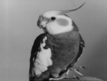
(a) Original Image

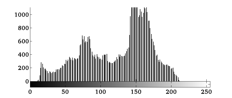
(b) Original histogram

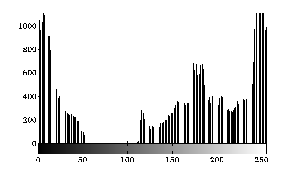
(c) Ring addition

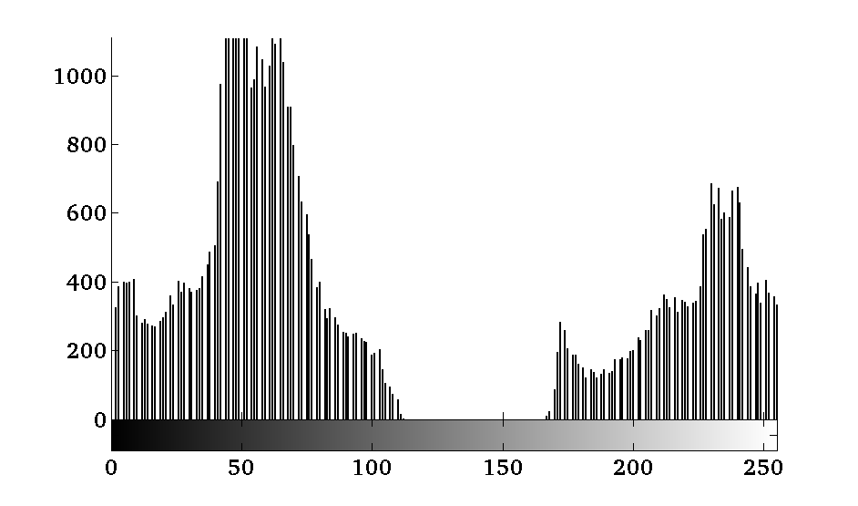
(d) Ring subtraction

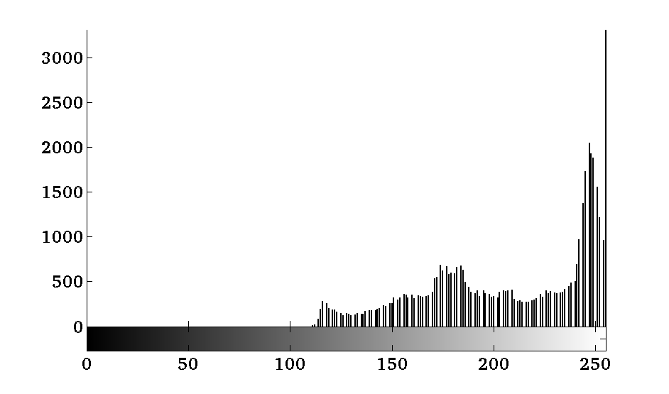
(e) Classical addition

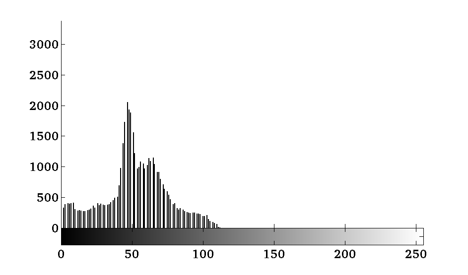
(f) Classical subtraction

Figure 2: A sample image and his histogram of frecuency.

Note that the effect of this operations only changes the value of the pixels but do not changes the frecuency or the number of gray levels. In fact, graphically it is possible to see that the addition or subtraction in the ring only generates a shift in the frequency histogram, so, the images with the frecuency histogram in Figure 2(c) and Figure 2(d), have the same properties and information that the original image in Figure 2(a). On the other hand, if we consider the classic addition and subtraction among images, it is easy to see in Figure 2(e) and Figure 2(f) that important information is lost due to the effect of truncation. In fact, this effect causes that high frequencies have been accumulated in $255$ in the addition case and in $0$ in the subtraction case (see Figures 2(e) and 2(f)).

Based on the above aspects, it is interesting to define the equivalence classes among images based on the concept of strong equivalence. This definition is necessary because the strong equivalent images has the same information, but from the point of view of intesity pixel, they do not have to be identically equal. In such sense, we will define the quotient group containing images in equivalent classes.

Definition 5 (Equivalence Classes)

Given an image $\mathcal{A}$, we said that the image $\mathcal{B}$ is in the class of $\mathcal{A}$ if and only if $\mathcal{A}$ and $\mathcal{B}$ are strongly equivalents. We denote the equivalence class of $\mathcal{A}$ as $C_{\mathcal{A}}$.

It is natural to consider the definition of the similarity index using the quotient space of the images by using strong equivalent images, considering the given equivalence classes above. For this reason, it is necessary to proof that the quotient space exists. More precisely, as strong equivalent images have been defined by the addition operation, the quotient group will be built on this operation.

Theorem 3.3

The set $N=\{\mathcal{S}\in G_{k\times m}(\mathbb{Z}_{n})(+,\cdot),\ S\ \mbox{is a scalar image}\}$ is a normal (or invariant) subgroup of $G_{k\times m}(\mathbb{Z}_{n})(+,\cdot)$.

Proof

First we will show that the set $N$ is a subgroup of $G_{k\times m}(\mathbb{Z}_{n})(+,\cdot)$.

1. Addition operation is well-defined. If $\mathcal{S},\ \mathcal{C}\in N\Rightarrow\forall\ i,j,i^{\prime},j^{\prime}(\ i,i^{\prime}\leq k\wedge j,j^{\prime}\leq m)$, $s_{i,j}=s_{i^{\prime},j^{\prime}}\wedge c_{i,j}=c_{i^{\prime},j^{\prime}}$ where $\{s_{i,j},\ s_{i^{\prime},j^{\prime}}\}$ are elements of $\mathcal{S}$ and $\{c_{i,j},\ c_{i^{\prime},j^{\prime}}\}$ are elements of $\mathcal{C}$. Then, $s_{i,j}+c_{i,j}=s_{i^{\prime},j^{\prime}}+c_{i^{\prime},j^{\prime}}$ and the image $\mathcal{S}+\mathcal{C}$ has all elements equals, so, $\mathcal{S}+\mathcal{C}\in N$.

2. Neutral element. The neutral element ($\mathcal{O}$) in the group is the image with all pixels equals to zero, defined at the previous subsection 3.1.

3. Inverse element. Let $\mathcal{S}\in N\Rightarrow\forall\ i,j,i^{\prime},j^{\prime},\ s_{i,j}=s_{i^{\prime},j^{\prime}}$, but $s_{i,j}\in\mathbb{Z}_{n}\Rightarrow s_{i,j}$ has a inverse element $s^{\prime}_{i,j}$ in $\mathbb{Z}_{n}$. Considering the image $\mathcal{S}^{\prime}$ with all elements equal to $s^{\prime}_{i,j}$, we obtain that $\mathcal{S}+\mathcal{S}^{\prime}=\mathcal{O}$, then $\mathcal{S}^{\prime}$ is the inverse of $\mathcal{S}$.

We have proved that $N$ is a subgroup of $G_{k\times m}(\mathbb{Z}_{n})(+,\cdot)$, only remains to prove that $N$ is normal. For this purpose we use that $N$ is a normal subgroup of $G$ if $\forall g\in G,\ g+N=N+g$ (see [17, 18, 19] for more details).

Let $\mathcal{A}\in\displaystyle\frac{G_{k\times m}(\mathbb{Z}_{n})(+,\cdot)}{N}$ and $\mathcal{S}\in N$, let us define $\mathcal{B}=\mathcal{A}+\mathcal{S}$ where $b_{i,j}=a_{i,j}+s_{i,j}\ \forall i,j$. But, we know that $\mathbb{Z}_{n}$ is abelian, therefore $G_{k\times m}(\mathbb{Z}_{n})(+,\cdot)$ is abelian too, so, $b_{i,j}=s_{i,j}+a_{i,j}\ \forall i,j,\Rightarrow\mathcal{B}=\mathcal{S}+\mathcal{A}$. Finally $\mathcal{A}+\mathcal{S}=\mathcal{S}+\mathcal{A}$.

With the last result, it was proved that the quotient space is well-defined, and it will be denoted by $\displaystyle\frac{G_{k\times m}(\mathbb{Z}_{n})(+,\cdot)}{N}$. Remember that the elements of this quotient space are the equivalence classes. Now, it does not matter which element of the class is chosen to carry out the operation, since any of these images are a representative element of its respective equivalence class.

Definition 6 (Natural Entropy Distance)

Let $C_{\mathcal{A}}$ and $C_{\mathcal{B}}$ be two elements in the quotient space $\displaystyle\frac{G_{k\times m}(\mathbb{Z}_{n})(+,\cdot)}{N}$, $\mathcal{A}_{1}\in C_{\mathcal{A}}$ and $\mathcal{B}_{1}\in C_{\mathcal{B}}$ are images. The Natural Entropy Distance (NED) between $\mathcal{A}_{1}$ and $\mathcal{B}_{1}$ is defined by

$$\hat{\nu}(\mathcal{A}_{1},\mathcal{B}_{1})=E(\mathcal{A}_{1}+(-\mathcal{B}_{1})).$$ (16)

The “Natural Entropy Distance” have the following properties related with the axioms of distance:

1. Non-Negativity: $\hat{\nu}(\mathcal{A}_{1},\mathcal{B}_{1})\geq 0$.
   Since entropy function is always positive, then

   $$\hat{\nu}(\mathcal{A}_{1},\mathcal{B}_{1})=E(\mathcal{A}_{1}+(-\mathcal{B}_{1}))\geq 0.$$

2. Identity of indiscernibles: $\hat{\nu}(\mathcal{A}_{1},\mathcal{B}_{1})=0\Leftrightarrow C_{\mathcal{A}}=C_{\mathcal{B}}$.

   $$\hat{\nu}(\mathcal{A}_{1},\mathcal{B}_{1})=0 \Leftrightarrow E(\mathcal{A}_{1}+(-\mathcal{B}_{1}))=0$$

   $$\Leftrightarrow \mathcal{A}_{1}+(-\mathcal{B}_{1})=\mathcal{S},\ \mathcal{S}\in N$$

   $$\Leftrightarrow \mathcal{B}_{1}\in C_{\mathcal{A}}$$

   $$\Leftrightarrow C_{\mathcal{A}}=C_{\mathcal{B}}.$$

3. Reflexivity: $\hat{\nu}(\mathcal{A}_{1},\mathcal{B}_{1})=\hat{\nu}(\mathcal{B}_{1},\mathcal{A}_{1})$.

   $$\hat{\nu}(\mathcal{A}_{1},\mathcal{B}_{1}) = E(\mathcal{A}_{1}+(-\mathcal{B}_{1}))$$

   $$= E(-(\mathcal{B}_{1}+(-\mathcal{A}_{1})))$$

   $$= E(\mathcal{B}_{1}+(-\mathcal{A}_{1}))$$

   $$= \hat{\nu}(\mathcal{B}_{1},\mathcal{A}_{1}).$$

If it are considered the images of Figure 1, applying the natural entropy distance the result shows that:

$$\hat{\nu}(Figure\ \ref{one_a},\ Figure\ \ref{two_b})=0.2514.$$

With this result, one can appreciate that have been differentiated images, including the spatial information too. The similarity index that was proposed in (16) is very simple and computationally efficient.

4 Natural Entropy Distance and $\mathit{MSHi}$

Taking in consideration the good properties that, in general, the NED definition has, one sees logical to take this new similarity index as the new stopping criterion of $\mathit{MSHi}$. Explicitly, the new stopping criterion is:

$$E(\mathcal{A}_{k}+(-\mathcal{A}_{k-1}))\leq\epsilon,$$ (17)

where $\epsilon$ and $k$ are respectively the threshold to stop the iterations and the number of iterations.

Since $\mathit{MSHi}$ is an iterative algorithm, we obtain a sequence that the processed image becames more homogenous as the algorithm advances. It is intuitive that comparing a resultant image $\mathcal{A}_{k}$ at a given iteration with the previous image $\mathcal{A}_{k-1}$ of the corresponding sequence, give us a measure about how much these images look like each other. The Algorithm 1 shows the general structure of the $\mathit{MSHi}$ with NED as stopping criterion. We denote this algorithm as $\mathit{MSHi}_{NED}$, and $\mathit{MSHi}_{WE}$ when the similarity index (15) is used as stopping criterion.

Data: Original Image ($\mathcal{A}$); Threshold to stop ($\epsilon$).

1 Initialize $\mathcal{B}_{1}=\mathcal{A}$ and $errabs=\infty$;

2 while $errabs>\epsilon$ do

•     

  Filter the original image according to the mean shift algorithm (Section 2.1);

store in $\mathcal{B}_{2}$ the filtered image;

Calculate using (17) the difference between $\mathcal{B}_{1}$ and $\mathcal{B}_{2}$, $errabs=\hat{\nu}(\mathcal{B}_{1},\mathcal{B}_{2})$. 4–      Update the images: $\mathcal{B}_{1}=\mathcal{B}_{2}$.

Result: $\mathcal{B}_{1}$ (is the segmented image).

Algorithm 1 $\mathit{MSHi}$ with Natural Entropy Distance ($\mathit{MSHi}_{NED}$)

The principal goal of this section is to evaluate the new stopping criterion in the $\mathit{MSHi}$ and to illustrate that, in general, with this new stopping criterion the algorithm has better stability in the segmentation process. For this aim, we used three different images for the experiments, which have been chosen according to the differences among their respective levels of high and low frequencies. The first image (“Bird”) has low frequencies, the second (“Baboon”) has high frequencies and in the image (“Montage”) has mixture low and high frequencies.

(a) Bird

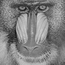
(b) Baboon

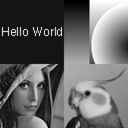
(c) Montage

Figure 3: Test images

All segmentation experiments were carried out by using a uniform kernel. In order to be effective the comparison between the old stopping criterion and the new stopping criterion, we use the same value of $h_{r}$ and $h_{s}$ in $\mathit{MSHi}$ ($h_{r}=12,\ h_{s}=15$). The value of $h_{s}$ is related to the spatial resolution of the analysis, while the value $h_{r}$ defines the range resolution. In the case of the new stopping criterion, we use the stopping threshold $\epsilon=0.9$ and when the old stopping criterion was used $\epsilon=0.01$.

Figure 4 shows the segmentation of the three images. Observe that, in all cases, the $\mathit{MSHi}$ had better result when the new stopping criterion was used.

Bird	Baboom	Montage

(a) $\mathit{MSHi}_{NED}$

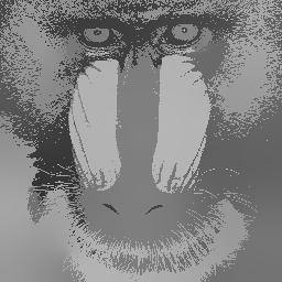
(b) $\mathit{MSHi}_{NED}$

(c) $\mathit{MSHi}_{NED}$

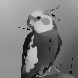
(d) $\mathit{MSHi}_{WE}$

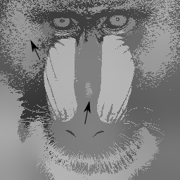
(e) $\mathit{MSHi}_{WE}$

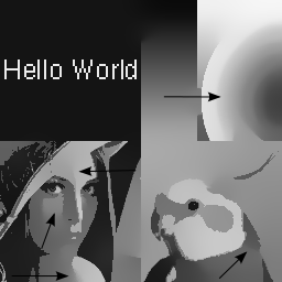
(f) $\mathit{MSHi}_{WE}$

Figure 4: Segmentation of the experimental images. In the first row are shown the segmentation using the new stopping criterion and in the secound row are the segmented images using the old stopping criterion.

When one compares Figures 4(a) and 4(d), in the part corresponding to the face or breast of the bird, more homogeneous area, with the new stopping criterion was obtained (see arrows in Figure 4(d)). Observe that, with the old stopping criterion the segmentation gives regions where different gray levels are originated. However, these regions really should have only one gray level. For example, Figure 4(b) and 4(e) show that the segmentation is more homogeneous when the new stopping criterion was used (see the arrows). In the case of the “Montage” image one can see that, in Figure 4(f) exists many regions that contains different gray levels when these regions really should have one gray level (see for example the face of Lenna, the circles and the breast of the bird). These good results are obtained because the defined new stopping criterion through the natural distance among images in expression (17) offers greater stability to the $\mathit{MSHi}$.

Figure 5 shows the profile of the obtained segmented images by using the two stopping criterion. The plates that appear in Figure 5(b) and 5(d) are indicative of equal intensity levels. In both graphics the abrupt falls of an intensity to other represent the different regions in the segmented image. Note that, in Figure 5(b) exists, in the same region of the segmentation, least variation of the pixel intensities with regard to Figure 5(d). This illustrates that, in this case the segmentation was better when the new stopping criterion was used.

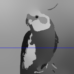
(a) New Criterion

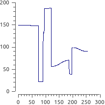
(b) Profile

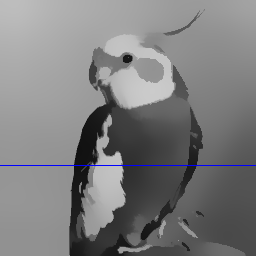
(c) Old Criterion

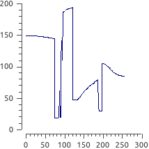
(d) Profile

Figure 5: An intensity profile through of a segmented image. Profile is indicated by a line. (a) and (c) are the segmented images and (b) and (d) are the profile of (a) and (c) respectively.

Figure 6 shows the performance of the two stopping criterion in the experimental images. In the “$x$” axis appears the iterations of $\mathit{MSHi}$ and in the “$y$” axis is shown the obtained values by the stopping criterion in each iteration of the algorithm.

Bird	Baboom	Montage

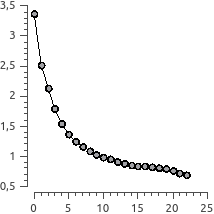
(a) $\mathit{MSHi}_{NED}$

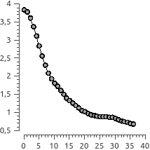
(b) $\mathit{MSHi}_{NED}$

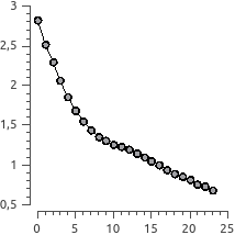
(c) $\mathit{MSHi}_{NED}$

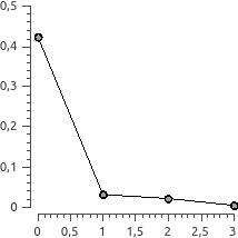
(d) $\mathit{MSHi}_{WE}$

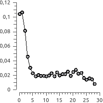
(e) $\mathit{MSHi}_{WE}$

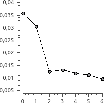
(f) $\mathit{MSHi}_{WE}$

Figure 6: Behavior of the stability of each algorithm according to the test images.

The graphics of iterations of the new stopping criterion (Figure 6(a), 6(b), 6(c)) show a smoother behavior; that is, the new stopping criterion has a stable performance through the $\mathit{MSHi}$. The new stopping criterion not only has good theoretical properties, but also, in the practice, has very good behavior.

On the other hand, if we analyze the old stopping criterion in the experimental images (Figure 6(d), 6(e), 6(f)), one can see that the performance in the $\mathit{MSHi}$ is unstable. In general, we have this type of situation when the stopping criterion defined in (15) is used. This can originate bad segmented images.

5 Conclusions

In this work, a new stopping criterion, for the iterative $\mathit{MSHi}$, based on the Ring Theory was proposed. The new stopping criterion establishes a new measure for the comparison of two images based on the use of the entropy concept and the spatial information. The quotient space was defined using the equivalent classes of images, to be able of selecting any element of the class. Through the obtained theoretical and practical results, it was possible to prove that the new stopping criterion had very good performance in the algorithm $\mathit{MSHi}$, and was more stable that the old criterion.

References

- [1] Y. Cheng, “Mean Shift, Mode Seeking, and Clustering”, IIEEE Trans. on Pattern Analysis and Machine Intelligence Ph. D. Thesis, New York University, 17 (8) (1995), pp. 790–799.
- [2] D. I. Comaniciu, “Nonparametric Robust Method for Computer Vision. ,”Ph. D. Thesis, Rutgers, The State University of New Jersey, (2000).
- [3] D. Comaniciu, P. Meer, “Mean Shift: A Robust Approach toward Feature Space Analysis”, IEEE Trans. on Pattern Analysis and Machine Intelligence Ph. D. Thesis, New York University, 24(5) (1974).
- [4] D. Dominguez and R. Rodriguez, “Convergence of the Mean Shift using the Linfinity Norm in Image Segmentation,” International Journal of Pattern Recognition Research, 1 (2011) pp. 3–4.
- [5] K. Fukunaga and L. D. Hostetler,, “The Estimation of the Gradient of a Density Function,” IEEE Trans. on Information Theory, IT-21(1) (1975) pp. 32–40.
- [6] T. Grenier, C. Revol-Muller, F. Davignon, and G. Gimenez, “Hybrid Approach for Multiparametric Mean Shift Filtering”, IEEE Image Processing, International Conference, Atlanta, GA, 17(8) (2006) pp. 8–11.
- [7] Y. Garces, E. Torres, O. Pereira, C. Perez, R. Rodriguez: Stopping Criterion for the Mean Shift Iterative Algorithm, Springer, Progress in Pattern Recognition, Image Analysis, Computer Vision, and Applications, Lecture Notes in Computer Science, Vol. 8258, pp. 383–390, 2013.
- [8] R. Rodriguez, E. Torres, and J. H. Sossa, “Image Segmentation based on an Iterative Computation of the Mean Shift Filtering for different values of window sizes,” International Journal of Imaging and Robotics, 6 (2011) pp. 1–19.
- [9] R. Rodriguez, A. G. Suarez, and J. H. Sossa, “A Segmentation Algorithm based on an Iterative Computation of the Mean Shift Filtering,” Journal Intelligent Robotic System, 63(3-4) (2011), pp. 447–463.
- [10] R. Rodriguez, E. Torres, and J. H. Sossa, “Image Segmentation via an Iterative Algorithm of the Mean Shift Filtering for Different Values of the Stopping Threshold,” International Journal of Imaging and Robotics, 63 (2012), pp. 1–19.
- [11] R. Rodriguez, “Binarization of medical images based on the recursive application of mean shift filtering: Another algorithm,” Journal of Advanced and Applications in Bioinformatics and Chemistry, Dove Medical Press, I (2008) pp. 1–12.
- [12] P. Suyash, and R. Whitake, “Higher-Order Image Statistics for Unsupervised, Information-Theoretic, Adaptive, Image Filtering”, IEEE Trans. on Pattern Analysis and Machine Intelligence, 28(3) 2006 pp. 364–376.
- [13] C. Shannon, “A Mathematical Theory of Communication”, Bell System Technology Journal, 24(5) (1948) pp. 370-423, pp. 623–656.
- [14] C. Shen, and M. J. Brooks, “Fast Global Kernel Density Mode Seeking: Applications to Localozation and Tracking”, IEEE Trans. on Image Processing, 16(5) 2007 pp. 1457–1469.
- [15] H. Zhang, J. E. Fritts and S. A. Goldma, “An Entropy-based Objective Evaluation Method for Image Segmentation, Storage and Retrieval Methods and Applications for Multimedia,” Proceeding of The SPIE, 5307 2003 pp. 38–49.
- [16] Wand, M., Jones, M.,“Kernel Smoothing”, Chapman and Hall, p. 95, 1995.
- [17] A. I. Kostrikin. “Introducción al Algebra”, Editorial Mir Moscu, 1983.
- [18] LIDL, Rudolf; Harald, Neiderreiter. “Introduction to finite fields and their applications”, Cambridge university press, 1994.
- [19] Noriega Sánchez, Teresita; Arazoza Rodríguez, Hector. “Algebra”, Editorial Félix Varela, vol. 2, 2003.