Flavour Physics and CP Violation in the Standard Model and Beyond

Abstract:

all

1 Introduction

We present the invited lectures given at the Third IDPASC School which took place in Santiago de Compostela in January 2013. The students attending the school had very different backgrounds, some of them were doing their PhD in experimental particle physics, others in theory. As a result, and in order to make the lectures useful for most of the students, we focused on basic topics of broad interest, avoiding the more technical aspects of Flavour Physics and CP Violation. We make a brief review of the Standard Model, paying special attention to the generation of fermion masses and mixing, as well as to CP violation. We describe some of the simplest extensions of the SM, emphasising novel flavour aspects which arise in their framework.

2 Review of the Standard Model

The Standard Model (SM) of unification of the electroweak and strong interactions [1, 2, 3, 4] is based on the gauge group

$$G_{\text{SM}}\equiv\mathsf{SU}(3)_{\text{\sc c}}\times\mathsf{SU}(2)_{\text{\sc l}}\times\mathsf{U}(1)_{\text{\sc y}}\,,$$ (1)

which has 12 generators. To each one of these generators corresponds a gauge field. The introduction of these gauge fields is essential in order to achieve invariance under local gauge transformations of $G_{\text{SM}}$. This is entirely analogous to what one encounters in electromagnetic interactions, where the photon is the gauge field associated to the $\mathsf{U}(1)_{\text{e.m.}}$, introduced in order to guarantee local gauge invariance. We shall denote the gauge fields in the following way:

$$\mathsf{SU}(3)_{\text{\sc c}}\, \longrightarrow\;G_{\mu}^{k},\;k=1,\dots,8\,;$$ (2)

$$\mathsf{SU}(2)_{\text{\sc l}}\, \longrightarrow\;W_{\mu}^{j},\;j=1,\dots,3\,;$$ (3)

$$\mathsf{SU}(2)_{\text{\sc l}}\, \longrightarrow\;B_{\mu}\,.$$ (4)

The electroweak interactions are linear combination of the following gauge bosons:

$$W_{\mu}^{a},\,B_{\mu}\;\longrightarrow\;W^{+}_{\mu},\,W^{-}_{\mu},\,Z_{\mu},\,A_{\mu}\,,$$ (5)

where $A_{\mu}$ is the photon field, mediator of electromagnetic interactions while the massive bosons $W^{+}_{\mu}$ and $Z_{\mu}$ mediate, respectively, the charged and neutral weak currents. Since $\mathsf{U}(1)_{\text{e.m.}}$ is a good symmetry of nature, the photon field should remain massless.

The SM describes all observed fermionic particles, which have definite gauge transformations properties and are replicated in three generations. All the SM fermionic fields carry weak hypercharge $Y$, defined as

$$Y\,\equiv\,Q-T_{3}\,,$$ (6)

where $Q$ is the electric charge operator and $T_{3}$ is the diagonal generator of $\mathsf{SU}(2)_{\text{\sc l}}$. Since experiments only provided evidence for left-handed charged currents, the right-handed components of fermion fields are put in $\mathsf{SU}(2)_{\text{\sc l}}$-singlets. Only the quarks carry colour, i.e they are triplets of $\mathsf{SU}(3)_{\text{\sc c}}$, while the leptons carry no colour. We summarise in Table 1 all fermionic content characterised by their transformation properties under the gauge group $\mathsf{SU}(3)_{\text{\sc c}}\,\times\,\mathsf{SU}(2)_{\text{\sc l}}\,\times\,\mathsf{U}(1)_{Y}$. It is worth noting that within this matter content the SM is free from anomalies, since $\mathsf{SU}(3)_{\text{\sc c}}$ is non-chiral, all representations of $\times\mathsf{SU}(2)_{\text{\sc l}}$ are real, the $\mathsf{SU}(3)^{2}\,Y$, $\mathsf{SU}(2)^{2}\,Y$ and $Y^{3}$ cancel between the quarks and leptons.

Table 1: The SM fermionic content. For a given SM representation $R$ one has $(n_{3},n_{2},y)\equiv(\dim_{\mathsf{SU}(3)}(R),\dim_{\mathsf{SU}(2)}(R),Y(R))\,.$ The index $i=1,2,3$ is the generation index.

${q_{i}}_{L}\equiv\begin{pmatrix}u_{i}\\ d_{i}\end{pmatrix}_{L}$	$(3,2,1/6)$
${u_{i}}_{R}$	$(3,1,2/3)$
${d_{i}}_{R}$	$(3,1,-1/3)$
${\ell_{i}}_{L}\equiv\begin{pmatrix}\nu_{i}\\ e^{-}_{i}\end{pmatrix}_{\text{\sc l}}$	$(1,2,-1/2)$
${e^{-}_{i}}_{R}$	$(1,1,-1)$

Gauge interactions are determined by the covariant derivative which is dictated by the transformation properties of the various fields, under the gauge group. In general one has

$$D_{\mu}\,=\,\partial_{\mu}-ig_{s}L^{k}G^{k}_{\mu}-igT^{j}W^{j}_{\mu}-ig^{\prime}y\,B_{\mu}\,,$$ (7)

where $T^{j}$ are the three $\mathsf{SU}(2)$-generators,

$$T^{j}\,=\,\left\{\begin{array}[]{cc}0\,,&\text{singlet}\\ \frac{\tau_{j}}{2}\,,&\text{fundamental}\end{array}\right.\,,$$ (8)

while $L^{k}$ are the eight $\mathsf{SU}(3)$-generators,

$$L^{k}\,=\,\left\{\begin{array}[]{cc}0\,,&\text{singlet}\\ \frac{\lambda_{k}}{2}\,,&\text{fundamental}\end{array}\right.\,.$$ (9)

The matrices $\tau_{j}$ and $\lambda_{k}$ are the usual Pauli and Gell-Mann matrices, respectively. For the fermions presented in Table 1 the covariant derivatives read as

$$D_{\mu}\,q_{L} =\left(\partial_{\mu}-i\frac{g_{s}}{2}\lambda_{k}\,G^{k}_{\mu}-i\frac{g}{2}\tau_{j}\,W^{j}_{\mu}-i\frac{g^{\prime}}{6}B_{\mu}\right)\,q_{L}\,,$$ (10)

$$D_{\mu}\,u_{R} =\left(\partial_{\mu}-i\frac{g_{s}}{2}\lambda_{k}\,G^{k}_{\mu}-i\frac{2g^{\prime}}{3}B_{\mu}\right)\,u_{R}\,,$$ (11)

$$D_{\mu}\,d_{R} =\left(\partial_{\mu}-i\frac{g_{s}}{2}\lambda_{k}\,G^{k}_{\mu}+i\frac{g^{\prime}}{3}B_{\mu}\right)\,d_{R}\,,$$ (12)

$$D_{\mu}\,\ell_{L} =\left(\partial_{\mu}-i\frac{g}{2}\tau_{j}\,W^{j}_{\mu}+i\frac{g^{\prime}}{2}B_{\mu}\right)\,q_{L}\,,$$ (13)

$$D_{\mu}\,e^{-}_{L} =\left(\partial_{\mu}+igB_{\mu}\right)\,e^{-}_{R}\,.$$ (14)

An important feature of the SM is the fact that right-handed neutrinos,

$$\nu_{R}\,\sim\,(1,1,0)\,,$$ (15)

are not introduced. As a result, neutrinos are strictly massless in the SM, in contradiction with present experimental evidence. We shall come back to this question in the sequel.

In order to account for the massive gauge bosons $W^{\pm}_{\mu}$ and $Z_{\mu}$ without destroying renormalisability, the gauge symmetry must be spontaneously broken. The simplest scheme to break spontaneously the electroweak gauge symmetry into electromagnetism, involves the introduction of a complex doublet Higgs scalar field $\phi$

$$\phi\,=\,\begin{pmatrix}\phi^{+}\\ \phi^{0}\end{pmatrix}\;\sim\;(1,2,1/2)\,,$$ (16)

which leads to the breaking:

$$\mathsf{SU}(3)_{\text{\sc c}}\times\mathsf{SU}(2)_{\text{\sc l}}\times\mathsf{U}(1)_{\text{\sc y}}\;\longrightarrow\;\mathsf{SU}(3)_{\text{\sc c}}\times\mathsf{U}(1)_{\text{e.m.}}\,.$$ (17)

The most general gauge invariant, renormalisable scalar potential is:

$$V(\phi)=\mu^{2}\phi^{\dagger}\phi\,+\,\lambda\left(\phi^{\dagger}\phi\right)^{2}\,.$$ (18)

Taking $\lambda>0$ the potential is bounded from below and two minima do exist. For $\mu^{2}>0$ one has $\langle 0|\phi|0\rangle=0$ while for $\mu^{2}<0$ one has instead

$$\langle 0|\phi|0\rangle\,=\,\begin{pmatrix}0\\ \frac{1}{\sqrt{2}}v\end{pmatrix}\,.$$ (19)

In Figure 1 it is drawn the Higgs potential around the two minima. Indeed, the case $\lambda>0$ and $\mu^{2}<0$ implies the spontaneous breaking of the electroweak gauge as indicated in eq. 17. One can check that the $\mathsf{U}(1)$ remains unbroken. The electric charge operator reads as

$$Q\,=\,T_{3}\,+\,Y\,,$$ (20)

and for the Higgs doublet one gets

$$Q\,=\,\begin{pmatrix}\frac{1}{2}&\ 0\ \\ \ 0\ &-\frac{1}{2}\end{pmatrix}\,+\,\begin{pmatrix}\frac{1}{2}&\ 0\ \\ \ 0\ &\frac{1}{2}\end{pmatrix}\,=\,\begin{pmatrix}\ 1\ &\ 0\ \\ 0&0\end{pmatrix}\,.$$ (21)

Therefore one verifies that the vacuum given in eq. (19) is invariant under the charge operator $Q$, since

$$Q\,\begin{pmatrix}0\\ \frac{1}{\sqrt{2}}v\end{pmatrix}\,=\,0\,,$$ (22)

and one gets

$$e^{i\,\alpha\,Q}\,\begin{pmatrix}0\\ \frac{1}{\sqrt{2}}v\end{pmatrix}\,=\,\bigg{[}1\,+\,i\,\alpha\,Q\,+\,\cdots\bigg{]}\,\begin{pmatrix}0\\ \frac{1}{\sqrt{2}}v\end{pmatrix}\,=\,\begin{pmatrix}0\\ \frac{1}{\sqrt{2}}v\end{pmatrix}\,.$$ (23)

Electric charge is automatically conserved in the SM. This is no longer true in extensions of the SM with two Higgs doublets, including the case of supersymmetric extensions of the SM. In the general two Higgs doublet model (2HDM) without loss of generality, one has:

$$\langle 0|\phi_{1}|0\rangle\,=\,\begin{pmatrix}0\\ \frac{1}{\sqrt{2}}v_{1}\end{pmatrix}\,,\qquad\langle 0|\phi_{2}|0\rangle\,=\,\begin{pmatrix}\xi\\ \frac{1}{\sqrt{2}}v_{2}\,e^{i\,\theta}\end{pmatrix}\,,$$ (24)

with $\xi$ real. In order to preserve charge conservation in the 2HDM, one has to choose a region of the parameter space where the minimum is at $\xi=0\,$.

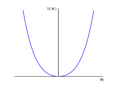
(a) $\lambda>0$,  $\mu^{2}>0$

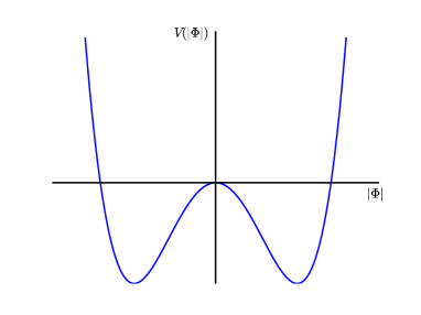
(b) $\lambda>0$,  $\mu^{2}<0$

Figure 1:

The SM does not provide an explanation for the charges of elementary fermions. The values of the hypercharge $Y$ are chosen in such a way that the correct electric charges are obtained. As an example, one can determined $Y_{q_{L}}\,$, by using the eq. (6) and the knowledge of $Q_{u}$ and $Q_{d}\,$. Thus,

$$Y_{u_{L}} =\,\frac{2}{3}-\frac{1}{2}\,=\,\frac{1}{6}\,,$$ (25)

$$Y_{d_{L}} =\,-\frac{1}{3}+\frac{1}{2}\,=\,\frac{1}{6}\,,$$ (26)

and therefore $Y_{q_{L}}=1/6\,$. It is rather intriguing the fact that the requirement of cancelation of the gauge anomaly in the SM together with the fact that the electromagnetic interactions are non-chiral is sufficient to fully determine all the hypercharges of the fundamental fermions up to an overall factor. In particular one gets relations among quark and lepton charges, leading to:

$$Q_{p}\,=\,-Q_{e}\,.$$ (27)

Although the hypercharge quantisation may arise from the anomaly-free condition, this is certainly not a satisfactory explanation in the SM. The solution to this fundamental question is elegantly answered in the framework of Grand-Unification, e.g. $\mathsf{SU}(5)$, where the quantisation of electric charges is related to some new phenomena like the magnetic monopoles predicted in the theory that can be tested in future experiments.

In order to describe the spontaneous breaking of the electroweak symmetry in the SM, one starts by introducing a convenient parametrisation of the Higgs doublet $\phi$ as

$$\phi\,=\,\begin{pmatrix}G^{+}\\ \frac{1}{\sqrt{2}}(v\,+\,H\,+\,i\,G_{0})\end{pmatrix}\,,$$ (28)

where $G^{+}$ is a charged complex scalar field, $H$ is a real scalar field and $G_{0}$ is a real pseudo-scalar. The scalar fields $G^{\pm}$ and $G_{0}$ are massless states, the so-called Nambu-Goldstone bosons. Through the Brout-Englert-Higgs mechanism, the charged bosons $G^{\pm}$ are absorbed as longitudinal components of the $W^{\pm}_{\mu}$ which acquire a mass:

$$M_{W}\,=\,\frac{g\,v}{2}\,,$$ (29)

while the neutral boson $G_{0}$ becomes the longitudinal component of the gauge boson $Z_{\mu}$, which is a linear combination of the bosons $B_{\mu}$ and $W^{3}_{\mu}$,

$$Z_{\mu}\,=\,\cos\theta_{W}\,W^{3}_{\mu}\,-\,\sin\theta_{W}\,B_{\mu}\,,$$ (30)

where $\theta_{W}$ is simply given by

$$\tan\theta_{W}\,\equiv\,\frac{g^{\prime}}{g}\,.$$ (31)

The $Z_{\mu}$ boson acquires then a mass given by

$$M_{Z}\,=\,\sqrt{g^{2}\,+\,g^{\prime 2}}\,\frac{v}{2}\,=\,\frac{M_{W}}{\cos\theta_{W}}\,.$$ (32)

The bosonic state orthogonal bosonic state to $Z_{\mu}$:

$$A_{\mu}\,=\,\cos\theta_{W}\,B_{\mu}\,+\,\sin\theta_{W}\,W^{3}_{\mu}\,,$$ (33)

remains massless and is identified with the photon. The electron coupling to the photon is directly determined from the weak couplings $g$ and $g^{\prime}$ as

$$\frac{1}{e^{2}}\,=\,\frac{1}{g^{2}}+\frac{1}{g^{\prime 2}}\,,$$ (34)

or

$$e=\frac{g\,g^{\prime}}{\sqrt{g^{2}+g^{\prime 2}}}\,=\,g\sin\theta_{W}\,=\,g^{\prime}\cos\theta_{W}\,.$$ (35)

3 Fermion masses and mixings

In the SM, one cannot write directly a mass term for any of the fundamental fermions because they would violate the gauge symmetry, since left-handed and right-handed chiralities do transform differently. The SM fermions acquire mass through Yukawa couplings, once the SM group is spontaneously broken. Therefore, in the SM the Higgs mechanism that is responsible for the breaking of the SM group, also generates fermion masses.

Quark and Charged Lepton masses

The Yukawa interactions are the most general terms in the Lagrangian allowed by the SM gauge group that involve fermions and the Higgs doublet. The Yukawa couplings can be written as:

$$-\mathrsfs{L}_{Y}\,=\,\left(Y_{u}\right)_{ij}\,\overline{q_{i}}_{L}\,\tilde{\phi}\,{u_{i}}_{R}\,+\,\left(Y_{d}\right)_{ij}\,\overline{q_{i}}_{L}\,\phi\,{d_{i}}_{R}\,+\,\left(Y_{\ell}\right)_{ij}\,\overline{\ell_{i}}_{L}\,\phi\,{e_{i}}_{R}\,+\,\text{H.c.}\,,$$ (36)

where $\tilde{\phi}\equiv\,i\tau_{2}\,\phi^{\dagger}$. The Yukawa matrices $Y_{u}$, $Y_{d}$ and $Y_{\ell}$ are arbitrary complex matrices in flavour space. The first two terms in eq. (36) will generate the up- and down-type quark masses while the third term will give rise to the charged lepton masses. Making use of the Higgs doublet parametrisation given in eq. (28) one can decompose the Lagrangian given in eq. (36) as

$$\begin{split}-\mathrsfs{L}_{Y}\,&=\,\frac{v}{\sqrt{2}}\,\left(Y_{u}\right)_{ij}\,\overline{u_{i}}_{L}\,{u_{i}}_{R}\,+\,\frac{v}{\sqrt{2}}\,\left(Y_{d}\right)_{ij}\,\overline{d_{i}}_{L}\,{d_{i}}_{R}\,+\,\frac{v}{\sqrt{2}}\,\left(Y_{\ell}\right)_{ij}\,\overline{e_{i}}_{L}\,{e_{i}}_{R}\\ &\,+\,\frac{\left(Y_{u}\right)_{ij}}{\sqrt{2}}\,\overline{u_{i}}_{L}\,{u_{i}}_{R}\,H\,+\,\frac{\left(Y_{d}\right)_{ij}}{\sqrt{2}}\,\overline{d_{i}}_{L}\,{d_{i}}_{R}\,H\,+\,\frac{\left(Y_{\ell}\right)_{ij}}{\sqrt{2}}\,\overline{e_{i}}_{L}\,{e_{i}}_{R}\,H\\ &\,-\,\frac{i\left(Y_{u}\right)_{ij}}{\sqrt{2}}\,\overline{u_{i}}_{L}\,{u_{i}}_{R}\,G^{0}\,+\,\frac{i\left(Y_{d}\right)_{ij}}{\sqrt{2}}\,\overline{d_{i}}_{L}\,{d_{i}}_{R}\,G^{0}\,+\,\frac{i\left(Y_{\ell}\right)_{ij}}{\sqrt{2}}\,\overline{e_{i}}_{L}\,{e_{i}}_{R}\,G^{0}\\ &\,-\,\left(Y_{u}\right)_{ij}\,\overline{d_{i}}_{L}\,{u_{i}}_{R}\,G^{-}\,+\,\left(Y_{d}\right)_{ij}\,\overline{u_{i}}_{L}\,{d_{i}}_{R},\,G^{+}\,+\,\left(Y_{\ell}\right)_{ij}\,\overline{\nu_{i}}_{L}\,{e_{i}}_{R}\,G^{+}\,+\,\text{H.c.}\,.\end{split}$$ (37)

Once a gauge transformation is performed in order to absorbed the Nambu-Goldstone bosons $G^{\pm}$ and $G^{0}$, the Lagrangian in eq. (37) becomes

$$\begin{split}-\mathrsfs{L}_{Y}\,&=\,\left(m_{u}\right)_{ij}\,\overline{u_{i}}_{L}\,{u_{i}}_{R}\,+\,\left(m_{d}\right)_{ij}\,\overline{d_{i}}_{L}\,{d_{i}}_{R}\,+\,\left(m_{\ell}\right)_{ij}\,\overline{e_{i}}_{L}\,{e_{i}}_{R}\\ &\,+\,\frac{\left(Y_{u}\right)_{ij}}{\sqrt{2}}\,\overline{u_{i}}_{L}\,{u_{i}}_{R}\,H\,+\,\frac{\left(Y_{d}\right)_{ij}}{\sqrt{2}}\,\overline{d_{i}}_{L}\,{d_{i}}_{R}\,H\,+\,\frac{\left(Y_{\ell}\right)_{ij}}{\sqrt{2}}\,\overline{e_{i}}_{L}\,{e_{i}}_{R}\,H\,+\,\text{H.c.}\,,\end{split}$$ (38)

where the quark mass matrices $m_{u}$, $m_{d}$ and the charged lepton mass matrix $m_{\ell}$ are simply defined by

$$m_{u}\,\equiv\,\frac{v}{\sqrt{2}}\,Y_{u}\,,\qquad m_{d}\,\equiv\,\frac{v}{\sqrt{2}}\,Y_{d}\,,\qquad m_{\ell}\,\equiv\,\frac{v}{\sqrt{2}}\,Y_{\ell}\,.$$ (39)

Gauge invariance does not constrain the flavour structure of Yukawa couplings and therefore $m_{u}$, $m_{d}$ and $m_{\ell}$ are arbitrary complex matrices.

Let us now focus on the mass terms,

$$-\mathrsfs{L}_{m}\,=\,\left(m_{u}\right)_{ij}\,{\overline{u_{i}}}^{0}_{L}\,{u^{0}_{i}}_{R}\,+\,\left(m_{d}\right)_{ij}\,{\overline{d_{i}}}^{0}_{L}\,{d^{0}_{i}}_{R}\,+\,\left(m_{\ell}\right)_{ij}\,{\overline{e_{i}}}^{0}_{L}\,{e^{0}_{i}}_{R}\,.$$ (40)

A super-script $0$ on the fermion fields was used that these fields are the original ones, in the weak basis. The matrices $m_{u,d,e}$ can be diagonalised by the following bi-unitary transformations:

$${u_{i}}^{0}_{L}\, =\,U_{L}^{u}\,{u_{i}}_{L}\,;\qquad{u_{i}}^{0}_{R}\,=\,U_{R}^{u}\,{u_{i}}_{R}\,,$$ (41a)

$${d_{i}}^{0}_{L}\, =\,U_{L}^{d}\,{d_{i}}_{L}\,;\qquad{d_{i}}^{0}_{R}\,=\,U_{R}^{d}\,{d_{i}}_{R}\,,$$ (41b)

$${e_{i}}^{0}_{L}\, =\,U_{L}^{e}\,{e_{i}}_{L}\,;\qquad{e_{i}}^{0}_{R}\,=\,U_{R}^{e}\,{e_{i}}_{R}\,,$$ (41c)

where $U^{u,d,e}_{R,L}$ are a set of unitary matrix such as

$$m_{u}\,\longrightarrow\,{U_{L}^{u}}^{\dagger}\,m_{u}\,U_{R}^{u}\, =\,\operatorname{diag}\left(m_{u},m_{c},m_{t}\right)\,,$$ (42a)

$$m_{d}\,\longrightarrow\,{U_{L}^{d}}^{\dagger}\,m_{d}\,U_{R}^{d}\, =\,\operatorname{diag}\left(m_{d},m_{s},m_{b}\right)\,,$$ (42b)

$$m_{\ell}\,\longrightarrow\,{U_{L}^{e}}^{\dagger}\,m_{\ell}\,U_{R}^{e}\, =\,\operatorname{diag}\left(m_{\ell},m_{\mu},m_{\tau}\right)\,.$$ (42c)

The fields $u_{L,R},d_{L,R},e_{L,R}$ are thus the mass eigenstates. The bi-unitary transformations given in eq. (41) affect the interactions between left-handed particles and the $W^{\pm}_{\mu}$ bosons - the charged currents - which are written in a weak basis as:

$$-\mathrsfs{L}_{\text{\sc cc}}\,=\,\frac{g}{\sqrt{2}}\left[{\overline{u_{i}}}^{0}_{L}\,\gamma^{\mu}\,{d_{i}}^{0}_{L}\,+\,{\overline{\nu_{i}}}^{0}_{L}\,\gamma^{\mu}\,{e_{i}}^{0}_{L}\right]\,W^{+}_{\mu}\,+\,\text{H.c.}\,.$$ (43)

In the mass eigenstate basis the charged currents become:

$$-\mathrsfs{L}_{\text{\sc cc}}\,=\,\frac{g}{\sqrt{2}}\left[\overline{u}_{L}\,\gamma^{\mu}\,{U_{L}^{u}}^{\dagger}U_{L}^{d}\,d_{L}\,+\,{\overline{\nu}}^{0}_{L}\,\gamma^{\mu}\,U_{L}^{e}\,e_{L}\right]\,W^{+}_{\mu}\,+\,\text{H.c.}\,.$$ (44)

The product of unitary matrices in eq. (44) defines the well know Cabibbo-Kobayshi-Maskawa matrix $V$ as

$$V\,\equiv\,{U_{L}^{u}}^{\dagger}U_{L}^{d}\,.$$ (45)

In the SM the unitary matrix $U_{L}^{e}$ is physically meaningless. Note that since neutrinos are massless in the SM, one can always redefine neutrino fields as

$$\nu^{0}_{L}\,\longrightarrow\,\nu_{L}\,=\,U_{L}^{e}\,{\nu}_{L}\,,$$ (46)

and therefore the charged current term ${\overline{\nu}}^{0}_{L}\,\gamma^{\mu}\,U_{L}^{e}\,e_{L}$ in eq. (44) becomes ${\overline{\nu}}_{L}\,\gamma^{\mu}\,e_{L}\,$. We then conclude that in the SM there is no leptonic mixing and therefore no neutrino oscillations.

We can show that the electromagnetic and neutral currents are not affected by the transformations given in eq. (41). The electromagnetic $J_{\text{e.m.}}$ given in the weak basis,

$$J^{\mu}_{\text{e.m.}}\,=\,\frac{2}{3}\,\left[\,\overline{u}^{0}_{L}\,\gamma^{\mu}\,u^{0}_{L}\,+\,\overline{u}^{0}_{R}\,\gamma^{\mu}\,u^{0}_{R}\,\right]\,-\frac{1}{3}\,\left[\,\overline{d}^{0}_{L}\,\gamma^{\mu}\,d^{0}_{L}\,+\,\overline{d}^{0}_{R}\,\gamma^{\mu}\,d^{0}_{R}\,\right]\,-\,\left[\,\overline{e}^{0}_{L}\,\gamma^{\mu}\,e^{0}_{L}\,+\,\overline{e}^{0}_{R}\,\gamma^{\mu}\,e^{0}_{R}\,\right]\,,$$ (47)

do not change in the mass eigenstate, since $J^{\mu}_{\text{e.m.}}$ transforms as

$$\begin{split}J^{\prime\mu}_{\text{e.m.}}\,=&\,\frac{2}{3}\,\left[\,\overline{u}_{L}\,\gamma^{\mu}\,{U_{L}^{u}}^{\dagger}U_{L}^{u}\,u_{L}\,+\,\overline{u}_{R}\,\gamma^{\mu}\,{U_{R}^{u}}^{\dagger}U_{R}^{u}\,u_{R}\,\right]\,-\frac{1}{3}\,\left[\,\overline{d}_{L}\,\gamma^{\mu}\,{U_{L}^{d}}^{\dagger}U_{L}^{d}\,d_{L}\,+\,\overline{d}_{R}\,\gamma^{\mu}\,{U_{R}^{d}}^{\dagger}U_{R}^{d}\,d_{R}\,\right]\\ \,-\,&\left[\,\overline{e}_{L}\,\gamma^{\mu}\,{U_{L}^{e}}^{\dagger}U_{L}^{e}\,e_{L}\,+\,\overline{e}_{R}\,\gamma^{\mu}\,{U_{R}^{e}}^{\dagger}U_{R}^{e}\,e_{R}\,\right]\,,\end{split}$$ (48)

and we get the same formal expression as in eq. (47). In a similar way we demonstrate that the neutral currents Lagrangian,

$$\mathrsfs{L}_{\text{\sc NC}}\,=\,\frac{g}{\cos\theta_{W}}\,\left[\,\overline{u}^{0}_{L}\,\gamma^{\mu}\,u^{0}_{L}\,-\,\overline{d}^{0}_{L}\,\gamma^{\mu}\,d^{0}_{L}\,+\,\,\overline{\nu}^{0}_{L}\,\gamma^{\mu}\,\nu^{0}_{L}\,-\,\overline{e}_{L}\,\gamma^{\mu}\,e^{0}_{L}\,-2\sin ˆ^{2}\theta_{W}\,J^{\mu}_{\text{e.m.}}\,\right]\,Z_{\mu}\,,$$ (49)

are also invariant under the transformations given in eq. (41).

$$\mathrsfs{L}^{\prime}_{\text{\sc NC}}\,=\,\frac{g}{\cos\theta_{W}}\,\left[\,\overline{u}_{L}\,\gamma^{\mu}\,u_{L}\,-\,\overline{d}_{L}\,\gamma^{\mu}\,d_{L}\,+\,\,\overline{\nu}_{L}\,\gamma^{\mu}\,\nu_{L}\,-\,\overline{e}_{L}\,\gamma^{\mu}\,e_{L}\,-2\sin ˆ^{2}\theta_{W}\,J^{\mu}_{\text{e.m.}}\,\right]\,Z_{\mu}\,.$$ (50)

Flavour changing neutral currents (FCNC) are naturally absent at three-level in the SM, due to the GIM mechanism. Indeed “charm” was invented in order to achieve this cancellation of FCNC.

Exercise 1

Suppose that “charm” did not exist, so that one would have

$$\begin{pmatrix}u_{1}^{0}\\ d_{1}^{0}\end{pmatrix}_{L}\,,\quad{d_{2}}_{L}\,,\quad{u_{1}}_{R}\,,\quad{d_{1}}_{R}\,,\quad\quad{d_{1}}_{R}\,.$$ (51)

Show that in this model FCNC automatically arise.

Historical note: Prior to the appearance of renormalisable gauge interactions, physicists considered the possibility that weak neutral currents could exist. However there was a strong prejudice against neutral currents due to the stringent experimental limits on the strength of FCNC.

Example 1

The decay $K^{0}_{L}\,\rightarrow\,\mu^{+}\,\mu^{-}$ has a branching ratio extremely suppressed, with respect to the decay $K^{0}_{L}\,\rightarrow\,\pi^{+}\,e^{-}\,\overline{\nu_{e}}\,$. If FCNC existed they would have branching ratios of the same order of magnitude which are shown in figure 2.

(a) $K^{0}_{L}\longrightarrow\pi^{+}e^{-}\nu_{e}$

(b) Does not exist at tree-level in SM

Figure 2:

From eq. (50) we see that neutral current interactions violate parity, since both couplings involving $\overline{\psi}\gamma_{\mu}\psi$ and $\overline{\psi}\gamma_{\mu}\gamma_{5}\psi$ are present.

As a result of the GIM mechanism there are no tree-level contributions to $K^{0}-\overline{K^{0}}$, $B^{0}-\overline{B^{0}}$, $B_{S}-\overline{B_{S}}$ and $D^{0}-\overline{D^{0}}$ mixings. However in the SM there are higher order contributions to these processes which are calculable. The contributions from the diagrams given in figure (3) led to the correct estimate to the charm quark mass [5] and the size of $B_{d}-\overline{B_{d}}$ mixing provided the first indirect evidence of a large top mass.

Exercise 2

Consider a simple extension of the SM which consists of the addition of an isosinglet quark $D$,

$$D_{L},D_{R}\,\sim\,(3,1,-1/3)\,.$$ (52)

1. Write down the most general quark mass terms which are obtained in the framework of this model.

2. Derive the structure of the charged currents.

3. Derive the structure of neutral currents, showing that there are FCNC in this model.

4. Show that although non-vanishing at tree level, FCNC are naturally suppressed in this model, provided the isosinglet quark $D$ is much heavier than the standard quarks.

Neutral currents have played a crucial rôle in the construction of the SM and its experimental tests and the discovery of Neutral weak currents was the first great success of the SM. As it was here described, the important feature of FCNC is that they are forbidden at tree-level, both in the SM and in most of its extensions. At loop level FCNC are generated and have played a crucial rôle in testing the SM and in putting bounds on New Physics beyond the SM through the study of process like: $K^{0}-\overline{K^{0}}$, $B^{0}-\overline{B^{0}}$, $B_{S}-\overline{B_{S}}$ and $D^{0}-\overline{D^{0}}$; rare kaon decays; rare b-meson decays; CP violation. In this framework, SM contributes to these processes at loop level and therefore New Physics has a chance to give significant contributions. On the other hand, the need to suppress FCNC has lead to two dogmas:

• no $Z$-mediated FCNC at tree level and no FCNC in the scalar sector, at tree level.

S. Glashow, S. Weimberg [6] and E.A. Paschos [7] derived necessary and sufficient conditions for having diagonal neutral currents, namely:

1. All quarks of fixed charge and helicity must transform according to the same irreducible representation of $\mathsf{SU}(2)$ and correspond to the same eigenvalue of $T_{3}$.

2. All quarks should receive their contributions to the quark mass matrix from a single neutral scalar VEV.

Can one violate the above two dogmas in reasonable extensions of the SM? The answer is yes!

“Reasonable” means that FCNC should be naturally suppressed without fine-tuning. In the gauge sector, the dogma can be violated through the introduction of a $Q=1/3$ and/or $Q=2/3$ vector-like quark [8, 9, 10, 11, 12, 13, 14], since in this model one has naturally small violation of $3\times 3$ unitarity of the CKM matrix $V$ which in turn leads to $Z$-mediated FCNC at tree level, which are naturally suppressed.

(a) $K^{0}-\overline{K^{0}}$ mixing

(b) $B^{0}_{d}-\overline{B^{0}_{d}}$ mixing

Figure 3:

In the Higgs sector, the dogma can be violated and yet having FCNC automatically suppressed by small CKM matrix elements [8].

Fundamental properties of the CKM matrix

We have introduced in eq. (45) the CKM matrix $V$, which characterises the flavour changing charged currents in the quark sector:

$$\mathrsfs{L}_{\text{CC}}\,=\,\begin{pmatrix}\overline{u}&\overline{c}&\overline{t}\end{pmatrix}_{L}\,\gamma^{\mu}\,\begin{pmatrix}V_{ud}&V_{us}&V_{ub}\\ V_{cd}&V_{cs}&V_{cb}\\ V_{td}&V_{ts}&V_{tb}\end{pmatrix}\,\begin{pmatrix}d\\ s\\ b\end{pmatrix}_{L}\,W_{\mu}^{+}\,\,+\,\text{H.c.}\,,$$ (53)

The CKM matrix is complex, but some of its phases have no physical meaning. This is due to the fact that one has the freedom to rephase the mass eigenstate quark fields $u_{\alpha}\,,d_{k}$:

$$u_{\alpha}\,=\,e^{i\,\varphi_{\alpha}}u^{\prime}_{\alpha}\,,\qquad d_{k}\,=\,e^{i\,\varphi_{k}}d^{\prime}_{k}\,.$$ (54)

Under this rephasing one has:

$$V_{\alpha k}^{\prime}\,=\,e^{i\,(\varphi_{k}-\varphi_{\alpha})}\,V_{\alpha k}\,.$$ (55)

It is clear from eq. (55) that the individual phases of $V_{ij}$ have no Physical meaning. It is useful to look for rephasing invariant quantities, which do not change under this rephasing. The simplest examples are moduli $|V_{\alpha k}|$ and quartets $Q_{\alpha i\beta j}$, defined as

$$Q_{\alpha i\beta j}\,\equiv\,V_{\alpha i}\,V_{\beta j}\,V^{*}_{\alpha j}\,V^{*}_{\beta i}\,,$$ (56)

with $\alpha\neq\beta$ and $i\neq j$. Invariants of higher order may in general be written as functions of the quartets and the moduli.

Exercise 3

Show that:

$$V_{\alpha i}\,V_{\beta j}\,V_{\gamma k}\,V^{*}_{\alpha j}\,V^{*}_{\beta k}\,V^{*}_{\gamma i}\,=\,\frac{Q_{\alpha i\beta j}\,Q_{\beta i\alpha j}}{|V_{\beta i}|^{2}}\,.$$ (57)

The quartets are easily constructed through the following scheme,

$$V\,=\,\leavevmode\hbox to121.96pt{\vbox to95.73pt{\text{[drawing]}}}\,, {V_{ud}} {V_{us}} {V_{ub}} {V_{cd}} {V_{cs}} {V_{cb}} {V_{td}} {V_{ts}} {V_{tb}} \left(\vbox{\hrule height=46.61557pt,depth=46.61557pt,width=0.0pt}\right. \left.\vbox{\hrule height=46.61557pt,depth=46.61557pt,width=0.0pt}\right) {V_{ud}} {V_{us}} {V_{ub}} {V_{cd}} {V_{cs}} {V_{cb}} {V_{td}} {V_{ts}} {V_{tb}} \left(\vbox{\hrule height=46.61557pt,depth=46.61557pt,width=0.0pt}\right. \left.\vbox{\hrule height=46.61557pt,depth=46.61557pt,width=0.0pt}\right)$$ (58)

where the two quartets,

$$V_{us}\,V_{cb}\,V^{*}_{ub}\,V^{*}_{cs}\,=\,Q_{uscb}\,,\qquad V_{cd}\,V_{ts}\,V^{*}_{td}\,V^{*}_{cs}\,=\,Q_{cdts}\,,$$ (59)

are illustrated. The diagonal dotted line refers to the product of the corresponding CKM elements.

3.1 Neutrino masses

In the SM, neutrinos are exactly massless. No Dirac mass terms can be written since right-handed neutrino fields are not introduced in the SM. On the other hand, Majorana mass terms are not generated in higher orders, due to exact $(B-L)$ conservation in the SM. As a result of having massless neutrinos, neither leptonic mixing nor leptonic CP violation can be generated in the SM. Indeed, any mixing arising from the diagonalisation of the charged-lepton masses can be rotated away by a redefinition of the neutrino fields.

In the view of above, one concludes that the discovery of leptonic mixing and non-vanishing neutrino masses, rules out the SM, as it was proposed. However a simple extension of the SM, sometimes denoted $\nu$SM, can easily accommodate leptonic mixing and provide an explanation for the smallness of neutrino masses, through the seesaw mechanism [15, 16, 17, 18, 19]. The nature of neutrinos (i.e. Majorana or Dirac) is still an important open question. Both in the case of Majorana [15, 16, 17, 18, 19] or Dirac neutrinos [20] one has to have a mechanism to understand the smallness of neutrino masses.

3.2 The Flavour sector of the SM

Let us now discuss the flavour sector of the SM. The gauge invariance does not constrain the flavour structure of the Yukawa matrices $Y_{u}$, $Y_{d}$ and using eq. (39) one obtains two arbitrary mass matrices $m_{u}$ and $m_{d}$. The two quark mass matrices are arbitrary complex matrices which need not to be Hermitian [21]. The two matrices $m_{u}$, $m_{d}$ contain $(18+18)$ parameters, but most of them are not physical. Due to the fermion family replication the gauge interaction part of $\mathrsfs{L}_{\text{SM}}$ has a very large flavour symmetry. One can make Weak-basis transformations which change $m_{u}$, $m_{d}$ but do not change the physical content of $m_{u}$, $m_{d}$. One has then a large redundancy in $m_{u}$, $m_{d}$. By making a WB transformation such as:

$$u^{0}_{L}\, =\,W_{L}\,{u^{0}_{L}}^{\prime}\,;\qquad u^{0}_{R}\,=\,W_{R}^{u}\,{u^{0}_{R}}^{\prime}\,,$$ (60a)

$$d^{0}_{L}\, =\,W_{L}\,{d^{0}_{L}}^{\prime}\,;\qquad d^{0}_{R}\,=\,W_{R}^{d}\,{d^{0}_{R}}^{\prime}\,,$$ (60b)

the gauge currents remain flavour diagonal but $m_{u}$, $m_{d}$ change as follows:

$$m_{u}\,\longrightarrow{m_{u}}^{\prime} =\,W_{L}^{\dagger}\,m_{u}\,W^{u}_{R}\,,$$ (61a)

$$m_{d}\,\longrightarrow{m_{d}}^{\prime} =\,W_{L}^{\dagger}\,m_{d}\,W^{d}_{R}\,,$$ (61b)

but the physical content does not change! Therefore, without loss of generality, one can make a WB transformation so that $m_{u}$ is diagonal, i.e. $m_{u}\,\operatorname{diag}(m_{u},\,m_{c},\,m_{t})$ and $m_{d}$ is Hermitian

$$m_{d}\,=\,\begin{pmatrix}m_{11}&m_{12}&m_{13}\\ m_{12}^{\ast}&m_{22}&m_{23}\\ m_{13}^{\ast}&m_{23}^{\ast}&m_{33}\end{pmatrix}\,.$$ (62)

In this basis, the only rephasing invariant phase is

$$\varphi\,\equiv\,\arg(m_{12}\,m_{23}\,m_{13}^{\ast})\,,$$ (63)

and there are ten independent parameters: 3 up-quark masses $m_{u},\,m_{c},\,m_{t}$, 6 moduli down-type matrix elements $|{m_{d}}_{ij}|$ and one rephasing invariant phase $\varphi$. There is to a difficulty in following a bottom-up approach in the search for a solution to the Flavour Puzzle: even if there is a Flavour Symmetry behind the spectrum or fermion masses and mixings, in what Weak-Basis will the symmetry be transparent? For example Texture Zeroes are Weak-Basis dependent [22].

3.3 CP Violation

In order to study the CP properties of a Lagrangian, it is convenient to separate the Lagrangian in two parts:

$$\mathrsfs{L}\,=\,\mathrsfs{L}_{(\text{CP})\,}\,+\,\mathrsfs{L}^{\prime}\,,$$ (64)

where $\mathrsfs{L}_{(\text{CP})\,}$ denotes the part of the Lagrangian which one knows that conserves CP. At this stage it is important to recall that a pure gauge Lagrangian is necessarily CP invariant [23]. One should allow for the most general CP transformations allowed by $\mathrsfs{L}_{\text{CP}}$. Typically, $\mathrsfs{L}_{\text{CP}}$ leaves a large freedom of choice in the definition of CP transformations. CP is violated if and only if there is no possible choice of CP transformation which leaves the Lagrangian invariant [24]. CP can be investigated in the fermion mass eigenstate or in a weak basis. We shall consider both cases. Let us study the CP properties of the SM, after spontaneous gauge symmetry breaking, and after diagonalisation of the quark mass matrices, i.e.,

$$m_{u}\, =\,\operatorname{diag}\left(m_{u},m_{c},m_{t}\right)\,,$$ (65a)

$$m_{d}\, =\,\operatorname{diag}\left(m_{d},m_{s},m_{b}\right)\,,$$ (65b)

which are non-degenerate. In the mass eigenstate basis, the most general CP transformation is:

$$(\text{CP})\,\,{W^{+}}^{\mu}(t,\vec{r})\,\,(\text{CP})^{-1} =\,-e^{i\zeta_{W}}{W^{-}}^{\mu}(t,-\vec{r})\,,$$ (66)

$$(\text{CP})\,\,{W^{-}}^{\mu}(t,\vec{r})\,\,(\text{CP})^{-1} =\,-e^{-i\zeta_{W}}{W^{+}}^{\mu}(t,-\vec{r})\,,$$

$$(\text{CP})\,\,u_{\alpha}(t,\vec{r})\,\,(\text{CP})^{-1} =\,e^{i\zeta_{\alpha}}\gamma^{0}\,C\,\overline{u}_{\alpha}^{\mathsf{T}}(t,-\vec{r})\,,$$

$$(\text{CP})\,\,d_{k}(t,\vec{r})\,\,(\text{CP})^{-1} =\,e^{i\zeta_{k}}\gamma^{0}\,C\,\overline{u}_{k}^{\mathsf{T}}(t,-\vec{r})\,,$$

where the conjugation matrix $C$ obeys to the relation $\gamma_{\mu}C=-C\gamma^{T}_{\mu}$. Invariance of charged current weak interactions under CP constrains $V_{\alpha k}$ to satisfy the following condition:

$$V_{\alpha k}^{*}\,=\,e^{i(\zeta_{W}+\zeta_{k}-\zeta_{\alpha})}\,V_{\alpha k}\,.$$ (67)

If one considers a single element of the $CKM$ matrix $V$, the previous condition can always be satisfied by using the freedom to choose $\zeta_{W},\zeta_{k},\zeta_{\alpha}\,$. However, it can be readily shown that the condition constrains all quartets and all rephasing invariant functions of $V$ to real. Therefore there is CP violation in the SM if and only if any of the rephasing invariant functions of the CKM matrix $V$ is not real.

In the SM with $n_{g}$ generations, the CKM matrix $V$ is a $n_{g}\times n_{g}$ unitary matrix and it can be then parametrised by $n_{g}^{2}$ independent parameters. Through rephasing of quark fields, one can remove $2\,n_{g}-1$ phases. Thus, the total number of parameters, denoted $N$, is given by

$$N\,=\,n_{g}^{2}-2\,n_{g}-1\,=\,(n_{g}-1)^{2}\,,$$ (68)

which shows that for three generations ($n_{g}=3$) one is left with 4 real parameters. If one takes into account that a unitary matrix is describe by $n_{g}(n_{g}-1)/2$ “angles”, one can further count the total number of physical phases $N_{ph}$ as:

$$N_{ph}\,=\,N-\frac{1}{2}n_{g}(n_{g}-1)\,=\,\frac{1}{2}(n_{g}-1)(n_{g}-2)\,.$$ (69)

We conclude that for 2 generations ($n_{g}=2$), there are no physical phases left and therefore CP is conserved. In the case of three generations ($n_{g}=3$), one has only one CP violating phase. There is another way of confirming this. For two generations, there is only one rephasing invariant quartet $Q_{udcs}$, defined as

$$Q_{udcs}\,\equiv\,V_{ud}\,V_{cs}\,V_{us}^{*}\,V_{cd}^{*}\,.$$ (70)

However using the orthogonality relation:

$$V_{ud}\,V_{cd}^{*}\,+\,V_{us}\,V_{cs}^{*}\,=\,0\,,$$ (71)

and multiplying by $V_{us}^{\ast}\,V_{cs}$, one obtains:

$$Q_{udcs}\,=\,-|V_{us}|^{2}\,|V_{cs}|^{2}\,,$$ (72)

which shows that $Q_{udcs}$ is real.

Figure 4: Unitarity triangle

Considering now the case of three generations, we see that orthogonality of the first two rows of $V$ leads to

$$V_{ud}\,V_{cd}^{*}\,+\,V_{us}\,V_{cs}^{*}\,+\,V_{ub}\,V_{cb}^{*}\,=\,0\,.$$ (73)

Multiplying by $V_{us}^{*}\,V_{cs}$ and taking imaginary parts one obtains:

$$\operatorname{Im}Q_{udcs}\,=\,-\operatorname{Im}Q_{ubcs}\,.$$ (74)

In an analogous way, one can show that for $n_{g}=3$ the imaginary parts of all quartets are equal, up to a sign. In the SM with three generations $|\operatorname{Im}Q|$ gives the strength of CP violation. If we consider the orthogonality between the first and third columns of $V$:

$$V_{ud}\,V_{ub}^{*}\,+\,V_{cd}\,V_{cb}^{*}\,+\,V_{td}\,V_{tb}^{*}\,=\,0\,.$$ (75)

This equation may be interpreted as a ”triangle” as represented in figure 4. One verifies easily that under rephasing, the triangle rotates. Therefore the orientation of the triangle has no physical meaning. Obviously, the internal angles of the triangles are rephasing invariant, namely

$$\alpha \equiv\,\arg\left[-V_{td}\,V_{ub}\,V_{ud}^{\ast}\,V_{tb}^{\ast}\right]\,=\,\arg(-Q_{ubtd})\,,$$ (76a)

$$\beta \equiv\,\arg\left[-V_{cd}\,V_{tb}\,V_{cb}^{\ast}\,V_{td}^{\ast}\right]\,=\,\arg(-Q_{tbcd})\,,$$ (76b)

$$\gamma \equiv\,\arg\left[-V_{ud}\,V_{cb}\,V_{ub}^{\ast}\,V_{cd}^{\ast}\right]\,=\,\arg(-Q_{cbud})\,,$$ (76c)

and one gets the following relation

$$\alpha\,+\,\beta\,+\,\gamma\,=\,\arg(-1)\,=\,\pi\pmod{\pi}\,.$$ (77)

This is true ”by definition”, and therefore it is not a test of unitarity!!

The quantity $\operatorname{Im}Q$ has a simple geometrical interpretation. It is twice the area of the unitarity triangles, as sketched in figure 4. The area of the triangles, $A$, is given by

$$A\,=\,\left|V_{cd}\,V_{cb}^{\ast}\right|\,\frac{h}{2}\,,$$ (78)

where the height of triangle, $h$, is given by

$$h\,=\,\left|V_{ud}\,V_{ub}^{\ast}\right|\,\sin\gamma\,,$$ (79)

with $\gamma$ defined in eq. (76c). One then obtains

$$A\,=\,\frac{1}{2}\left|\operatorname{Im}Q_{udcb}\right|\,.$$ (80)

Since all $|\operatorname{Im}Q|$ are equal then all triangles have the same area.

Experimentally we know that:

$$\left|V_{\rm{CKM}}\right|\,\simeq\,\begin{pmatrix}1&\lambda&\lambda^{3}\\ \lambda&1&\lambda^{2}\\ \lambda^{3}&\lambda^{2}&1\end{pmatrix}\,,$$ (81)

with $\lambda\approx 0.22$.

The six unitarity triangles are given by

$$\stackrel{{\scriptstyle\lambda}}{{V_{ud}\,V_{us}^{\ast}}}\,+\,\stackrel{{\scriptstyle\lambda}}{{V_{cd}\,V_{cs}^{\ast}}}\,+\,\stackrel{{\scriptstyle\lambda^{5}}}{{V_{td}\,V_{ts}^{\ast}}} =\,0\,,\qquad T_{ds}$$ (82)

$$\stackrel{{\scriptstyle\lambda^{3}}}{{V_{ud}\,V_{ub}^{\ast}}}\,+\,\stackrel{{\scriptstyle\lambda^{3}}}{{V_{cd}\,V_{cb}^{\ast}}}\,+\,\stackrel{{\scriptstyle\lambda^{3}}}{{V_{td}\,V_{tb}^{\ast}}} =\,0\,,\qquad T_{db}$$

$$\stackrel{{\scriptstyle\lambda^{4}}}{{V_{us}\,V_{ub}^{\ast}}}\,+\,\stackrel{{\scriptstyle\lambda^{2}}}{{V_{cs}\,V_{cb}^{\ast}}}\,+\,\stackrel{{\scriptstyle\lambda^{2}}}{{V_{ts}\,V_{tb}^{\ast}}} =\,0\,,\qquad T_{sb}$$

$$\stackrel{{\scriptstyle\lambda}}{{V_{ud}\,V_{cd}^{\ast}}}\,+\,\stackrel{{\scriptstyle\lambda}}{{V_{cs}\,V_{cs}^{\ast}}}\,+\,\stackrel{{\scriptstyle\lambda^{5}}}{{V_{ub}\,V_{cb}^{\ast}}} =\,0\,,\qquad T_{uc}$$

$$\stackrel{{\scriptstyle\lambda^{3}}}{{V_{ud}\,V_{td}^{\ast}}}\,+\,\stackrel{{\scriptstyle\lambda^{3}}}{{V_{us}\,V_{ts}^{\ast}}}\,+\,\stackrel{{\scriptstyle\lambda^{3}}}{{V_{ub}\,V_{td}^{\ast}}} =\,0\,,\qquad T_{ut}$$

$$\stackrel{{\scriptstyle\lambda^{4}}}{{V_{cd}\,V_{td}^{\ast}}}\,+\,\stackrel{{\scriptstyle\lambda^{2}}}{{V_{cs}\,V_{ts}^{\ast}}}\,+\,\stackrel{{\scriptstyle\lambda^{2}}}{{V_{tb}\,V_{tb}^{\ast}}} =\,0\,,\qquad T_{ct}$$

Let us now comment on the strength of CP violation in the SM, which

$$\left|\operatorname{Im}Q\right|\,=\,\left|\,\stackrel{{\scriptstyle\lambda^{0}}}{{V_{ud}}}\,\stackrel{{\scriptstyle\lambda^{3}}}{{V_{ub}}}\,\stackrel{{\scriptstyle\lambda}}{{V_{cd}}}\,\stackrel{{\scriptstyle\lambda^{2}}}{{V_{cb}}}\,\right|\,\sin\gamma\,.$$ (83)

In order to account for CP violation in the kaon sector, $\sin\gamma$ should be of order 1. So $|\operatorname{Im}Q|\approx\lambda^{6}$.

The strength of CP violation (measured by $\operatorname{Im}Q$) is small in the SM, due to the smallness of some CKM moduli $|V_{ij}|$, like $|V_{ub}|$, $|V_{cb}|$. What would be the maximal possible value of $\operatorname{Im}Q$? The maximal value is obtained for the following mixing matrix with universal moduli as

$$V\,=\,\frac{1}{\sqrt{3}}\,\begin{pmatrix}1&1&1\\ 1&\omega&\omega^{\ast}\\ 1&\omega^{\ast}&\omega\end{pmatrix}\,,$$ (84)

with $\omega\equiv\exp(i2\pi/3)\,$, yielding

$$\operatorname{Im}Q\,=\,\frac{1}{6\sqrt{3}}\,\approx\,0.096\,.$$ (85)

A convenient parametrisation of the CKM matrix is the so-called Standard Parametrisation, which is defined by the product of three rotations, namely:

$$\begin{split}V(\theta_{12},\theta_{13},\theta_{23},\delta_{13})&\,=\,\begin{pmatrix}1&0&0\\ 0&c_{23}&s_{23}\\ 0&-s_{23}&c_{23}\end{pmatrix}\begin{pmatrix}c_{13}&0&s_{13}\,e^{-i\delta_{13}}\\ 0&1&0\\ -s_{13}\,e^{i\delta_{13}}&0&c_{13}\end{pmatrix}\begin{pmatrix}c_{12}&s_{12}&0\\ -s_{12}&c_{12}&0\\ 0&0&1\end{pmatrix}\\ \,=\,&\begin{pmatrix}c_{12}\,c_{13}&s_{12}\,c_{13}&s_{13}\,e^{-i\delta_{13}}\\ -s_{12}\,c_{23}-c_{12}\,s_{23}\,s_{13}e^{i\delta_{13}}&c_{12}\,c_{23}-s_{12}\,s_{23}\,s_{13}e^{i\delta_{13}}&s_{23}\,c_{13}\\ s_{12}\,s_{23}-c_{12}\,c_{23}\,s_{13}e^{i\delta_{13}}&-c_{12}\,s_{23}-s_{12}\,c_{23}\,s_{13}e^{i\delta_{13}}&c_{23}\,c_{13}\end{pmatrix}\,,\end{split}$$ (86)

where $c_{ij}\equiv\cos\theta_{ij}$ and $s_{ij}\equiv\sin\theta_{ij}$. One of the advantages of the Standard Parametrisation is that the $s_{ij}$ are simply related to directly measured quantities:

$$s_{13}\,=\,|V_{ub}|\,,\qquad s_{12}\,=\,\frac{|V_{us}|}{\sqrt{1-|V_{ub}|^{2}}}\,,\qquad s_{23}\,=\,\frac{|V_{cb}|}{\sqrt{1-|V_{ub}|^{2}}}\,.$$ (87)

Once $s_{ij}$ are fixed, all data has to be fit by a single parameter: $\delta_{13}\,$.

Invariant Approach to CP Violation

In this section we review the invariant approach to CP violation [25]. As previously indicated we write $\mathrsfs{L}$ as in eq. (64). In order to analyse whether the whole Lagrangian violates CP, one has to check whether the CP transformation under which $\mathrsfs{L}_{(\text{CP})\,}$ is invariant implies non-trivial restrictions, i.e. restrictions which may not be satisfied by $\mathrsfs{L}^{\prime}\,$ defined in eq. (64). In the case of the SM, the most general CP transformations which leave $\mathrsfs{L}_{(\text{CP})\,}$ invariant are:

$$(\text{CP})\,\,u_{L}^{0}\,\,(\text{CP})^{-1} =\,e^{i\zeta_{W}}\,K_{L}\,\gamma^{0}\,C\,\overline{u^{0}_{L}}^{\mathsf{T}}\,,$$ (88)

$$(\text{CP})\,\,d_{L}^{0}\,\,(\text{CP})^{-1} =\,K_{L}\,\gamma^{0}\,C\,\overline{d^{0}_{L}}^{\mathsf{T}}\,,$$

$$(\text{CP})\,\,u_{R}^{0}\,\,(\text{CP})^{-1} =\,K^{u}_{R}\,\gamma^{0}\,C\,\overline{u^{0}_{R}}^{\mathsf{T}}\,,$$

$$(\text{CP})\,\,d_{R}^{0}\,\,(\text{CP})^{-1} =\,K^{d}_{R}\,\gamma^{0}\,C\,\overline{d^{0}_{R}}^{\mathsf{T}}\,,$$

where $K_{L}$, $K^{u}_{L}$ and $K^{d}_{R}$ are unitary matrices acting in flavour space. It can be shown that in order for the Yukawa interactions (or equivalently $m_{u}\,,m_{d}$) to be CP invariant, the following relations have to be satisfied:

$$K^{\dagger}_{L}\,m_{u}\,K^{u}_{R} =m^{\ast}_{u}\,,$$ (89)

$$K^{\dagger}_{L}\,m_{d}\,K^{d}_{R} =m^{\ast}_{d}\,.$$

The existence of the matrices $K_{L}$, $K^{u}_{L}$ and $K^{d}_{R}$ is a necessary and sufficient condition for CP invariance in the SM.

Exercise 4

Prove the above result.

It is rather convenient to define the Hermitian matrices $H_{u}$,$H_{d}$ as:

$$H_{u}\,\equiv\,m_{u}\,m^{\dagger}_{u}\,,\qquad H_{d}\,\equiv\,m_{d}\,m^{\dagger}_{d}\,.$$ (90)

Thus, from eq. (89) one derives:

$$K^{\dagger}_{L}\,H_{u}\,K_{L} =\,H^{\ast}_{u}\,=\,H^{\mathsf{T}}_{u}\,,$$ (91)

$$K^{\dagger}_{L}\,H_{d}\,K_{L} =\,H^{\ast}_{u}\,=\,H^{\mathsf{T}}_{u}\,,$$

and therefore one has

$$K^{\dagger}_{L}\,[H_{u},H_{d}]\,K_{L}\,=\,[H_{u}^{\mathsf{T}},H_{d}^{\mathsf{T}}]\,=\,-[H_{u},H_{d}]^{\mathsf{T}}\,.$$ (92)

Taking the trace of an odd $r$ power of the above equation we find

$$\operatorname{Tr}[H_{u},H_{d}]^{r}\,=\,0\,.\qquad(r\;\,\rm{odd})$$ (93)

Therefore, one concludes that in the SM CP invariance implies $\operatorname{Tr}[H_{u},H_{d}]^{r}\,=\,0\,$. For the case of $r=1$ this relation is trivially satisfied, since the trace of a commutator is automatically zero. The minimum non-trivial case is for $r=3$. Note that eq. (93) is a necessary condition for CP invariance for any number of generations. For two generations the invariant automatically vanishes. In the case of three generations one obtains:

$$\begin{split}\operatorname{Tr}[H_{u},H_{d}]^{3}=6i&(m^{2}_{t}-m^{2}_{c})(m^{2}_{t}-m^{2}_{u})(m^{2}_{c}-m^{2}_{u})\\ &(m^{2}_{b}-m^{2}_{s})(m^{2}_{b}-m^{2}_{d})(m^{2}_{s}-m^{2}_{d})\,\operatorname{Im}Q.\end{split}$$ (94)

It can be shown [25] that the vanishing of $\operatorname{Tr}[H_{u},H_{d}]^{3}$ is a necessary and sufficient condition for CP invariance in the SM with three generations. For more than three generations the vanishing of this invariant continuous being a necessary condition for CP invariance, but no longer is a sufficient condition. In the case of three generations one has:

$$\det[H_{u},H_{d}]\,=\,\frac{1}{3}\,tr[H_{u},H_{d}]^{3}\,,$$ (95)

and thus the vanishing of the above determinant can be used [26] as a necessary and sufficient condition for CP invariance. .

Exercise 5

Prove the above result given by eq. (94). Hint: choose to work in a weak basis where either $H_{u}$ or $H_{d}$ is diagonal.

4 Physics Beyond the Standard Model

4.1 Neutrino Masses

It was already mentioned that in the SM, neutrinos are strictly massless. There are no Dirac mass terms since no fermionic right-handed field $\nu_{R}$ is not introduced. There are no Majorana mass terms at tree level, since no scalar $\mathsf{SU}(2)$-triplet is introduced. Also no Majorana mass is generated at higher orders, due to exact $B-L$ conservation. Note that the Majorana mass term:

$$\nu_{L}^{\mathsf{T}}\,C\,\nu_{L}\,,$$ (96)

violates $B-L$ by 2 units. The same applies to $\mathsf{SU}(5)$ GUT, where $B-L$ is also an accidental symmetry.

It can be readily seen that in the SM, there is no leptonic mixing. The leptonic charged currents is given by

$$\overline{\nu}^{0}_{Li}\,\gamma^{\mu}\,\ell^{0}_{Li}\,W_{\mu}\,,$$ (97)

where $\nu^{0}_{Li}$ and $\ell^{0}_{Li}$ are weak eigenstates. After diagonalisation of the charged lepton mass matrix the leptonic charged currents become

$$\overline{\nu}^{0}_{L}\,\gamma^{\mu}\,U\,\ell_{L}\,W_{\mu}\,,$$ (98)

where $\ell_{L}$ is now in the mass eigenstate. But the unitary matrix $U$ can be eliminated through a redefinition of $nu^{0}_{L}$ so that the charged currents become flavour diagonal:

$$\overline{\nu}_{L}\,\gamma^{\mu}\,\ell_{L}\,W_{\mu}\,.$$ (99)

Observation of neutrino oscillations provides clear evidence for New Physics beyond the SM. The Minimal extension of the SM which allows for non-vanishing neutrino masses introduces right-handed neutrino fields, $\nu_{Ri}$, a ”strange” missing feature of the SM. Once the right-handed neutrino fields are introduced, Dirac masses for neutrinos are generated. Yukawa interactions can then be written as

$${(Y_{\nu})}_{ij}\,\overline{\ell}_{i}\,\tilde{\phi}\,\nu_{Ri}\,+\,\text{H.c.}\,,$$ (100)

where the Yukawa mass matrix $Y_{\nu}$ is arbitrarily complex. After the spontaneous breaking of the electroweak gauge symmetry Dirac neutrino masses are then generated as

$$m_{D}\,=\,{(Y_{\nu})}_{ij}\,\frac{v}{\sqrt{2}}\,.$$ (101)

If one writes the most general Lagrangian consistent with gauge invariance and renormalisability, one has to include the mass term:

$${(M_{R})}_{ij}\,\nu_{Ri}^{\mathsf{T}}\,C\,\nu_{Rj}\,,$$ (102)

where $M_{R}$ is a symmetric complex matrix. One may have $M_{R}\gg v$, since the mass term is gauge invariant. This leads to the seesaw mechanism, with:

$$(m_{\nu})_{\text{light}}\, \approx\,\frac{v^{2}}{M_{R}}\,,$$ (103a)

$$(M)_{\text{heavy}}\, \approx\,M_{R}\,.$$ (103b)

Note that this minimal extension of the SM, sometimes denoted $\nu$SM, is actually ”simpler” and more ”natural” than the SM, providing a simple and plausible explanation for the smallness of neutrino masses.

For the moment let us consider the low energy limit of the $\nu$SM. Let us consider the neutrino masses and mixing at low energies, i.e the mass term Lagrangian

$$\mathrsfs{L}_{\text{mass}}\,=\,-\overline{\ell}_{L}\,m_{\ell}\,\ell_{R}\,-\,\frac{1}{2}\nu_{L}^{\mathsf{T}}\,C\,m_{\nu}\,\nu_{L}\,+\,\text{H.c.}\,,$$ (104)

and the charged current Lagrangian

$$\mathrsfs{L}_{W}\,=\,\frac{g}{\sqrt{2}}\,\overline{\ell}_{L}\,\gamma^{\mu}\,\nu_{L}\,W_{\mu}\,+\,\text{H.c.}\,,$$ (105)

where $m_{\ell}$, an arbitrary complex matrix, and $m_{\nu}$, a symmetric complex matrix, encode all information about lepton masses and mixing. There is a great redundancy in $m_{\ell}$, $m_{\nu}$, since not all their parameters are physical. This redundancy stems from the freedom to make Weak-Basis transformations:

$$\nu_{L}=W_{L}\,\nu_{L}\textasciiacute\,,\qquad\ell_{L}=W_{L}\,\ell_{L}\textasciiacute\,,\qquad\ell_{R}=W_{R}\,\ell_{R}\textasciiacute\,,$$ (106)

where $W_{L}$, $W_{L}$ are unitary matrices. The matrices $m_{\ell}$, $m_{\nu}$ transform then as:

$$m^{\prime}_{\ell}\,=\,W^{\dagger}_{L}\,m_{\ell}\,W_{R}\,,\qquad m^{\prime}_{\nu}\,=\,W^{\mathsf{T}}_{L}\,m_{\nu}\,W_{L}\,.$$ (107)

One can use the freedom to make WB transformations to go to a basis where

$$m_{\ell}\,=\,d_{\ell}$$ (108)

is diagonal and real. In this basis, one can still make a rephasing:

$$\ell_{L,R}^{\prime\prime}=K_{L}\,\ell_{L,R}\textasciiacute\,,\qquad\nu^{\prime\prime}_{L}=K_{L}\,\nu_{L}\textasciiacute\,,$$ (109)

with $K_{L}\,=\,\operatorname{diag}(e^{i\,\varphi_{1}},\,e^{i\,\varphi_{2}},\,e^{i\,\varphi_{3}})\,$. Under this rephasing $d_{\ell}$ remains invariant, but $m_{\nu}$ transforms as:

$$\left(m_{\nu}^{\prime\prime}\right)_{ij}\,=\,e^{i\,(\varphi_{i}\,+\,\varphi_{j})}\,\left(m_{\nu}^{\prime}\right)_{ij}\,.$$ (110)

One can eliminate $n$ phases from $m_{\nu}$. The number of physical phases in $m_{\nu}$ is:

$$N_{ph}\,=\,\frac{1}{2}\,n(n+1)-n\,=\,\frac{1}{2}\,n(n-1)\,,$$ (111)

where $n$ is the number of right-handed neutrino fields. For $n=3$ one has $N_{ph}=3$. So altogether one has in $m_{\nu}$: 6 real moduli $|(m_{\nu}^{\prime\prime})_{ij}|$ and three phases ($N_{ph}=3$). The individual phases of $(m_{\nu}^{\prime\prime})_{ij}$ have no physical meaning because they are not rephasing invariant. But one can construct polynomials of $(m_{\nu}^{\prime\prime})_{ij}$ which are rephasing invariant. Examples of rephasing invariant polynomials:

$$P_{1} \,\equiv\,(m_{\nu}^{\ast})_{11}(m_{\nu}^{\ast})_{22}(m_{\nu})^{2}_{12}\,,$$ (112)

$$P_{2} \,\equiv\,(m_{\nu}^{\ast})_{11}(m_{\nu}^{\ast})_{33}(m_{\nu})^{2}_{13}\,,$$

$$P_{3} \,\equiv\,(m_{\nu}^{\ast})_{33}(m_{\nu}^{\ast})_{12}(m_{\nu})_{13}(m_{\nu})_{23}\,.$$

Let us now discuss the generation of the leptonic mixing in the charged current. The charged leptonic mass matrix is diagonalised as

$$U_{eL}^{\dagger}m_{\ell}\,U_{eR}\,=\,\operatorname{diag}(m_{e}\,,m_{\mu}\,,m_{\tau})\,,$$ (113)

through the unitary matrices $U_{eL}\,$, $U_{eL}\,$, while the effective neutrino mass matrix is diagonalised as

$$U_{\nu}^{\mathsf{T}}\,m_{\nu}\,U_{\nu}\,=\,\operatorname{diag}(m_{1}\,,m_{2}\,,m_{3})\,.$$ (114)

through the unitary matrix $U_{\nu}\,$. Under these unitary transformations the charged currents are

$$\mathrsfs{L}_{W}\,=\,\frac{g}{\sqrt{2}}\,\overline{\ell}_{L}\,\gamma^{\mu}\,U\,\nu_{L}\,W_{\mu}\,+\,\text{H.c.}\,.$$ (115)

The unitary matrix $U$, which measure the mixing in the leptonic sector, given by

$$U\,\equiv\,U_{\ell}^{\dagger}\,U_{\nu}\,,$$ (116)

is the so-called the Pontecorvo-Maki-Nakagawa-Sakata (PMNS) [27, 28, 29] matrix. In this basis, there is still freedom to rephase the charged lepton fields

$$\ell_{j}\,\longrightarrow\,\ell^{\prime}_{j}\,=\,\\ exp(,i\,\phi_{j}),\ell_{j}\,,$$ (117)

with arbitrary phases $\phi_{j}$. Due to the Majorana nature of neutrinos, the rephasing:

$$\nu_{Lk}\,\longrightarrow\,\nu^{\prime}_{Lk}\\ ,=\,\\ exp(,i\,\psi_{j}),\nu_{Lk}\,,$$ (118)

with arbitrary phases $\psi_{k}$, is not allowed, since it would not leave the Majorana mass terms

$$\nu_{Lk}^{\mathsf{T}}\,C\,m_{k}\,\,\nu_{Lk}\,,$$ (119)

invariant. In the mass eigenstate basis, the charred currents are

$$\mathrsfs{L}_{W}\,=\,\frac{g}{\sqrt{2}}\,\begin{pmatrix}\overline{e}&\overline{\mu}&\overline{\tau}\end{pmatrix}_{L}\,\gamma^{\mu}\,\begin{pmatrix}U_{e1}&U_{e2}&U_{e3}\\ U_{\mu 1}&U_{\mu 2}&U_{\mu 3}\\ U_{\tau 1}&U_{\tau 2}&U_{\tau 3}\end{pmatrix}\,\begin{pmatrix}\nu_{1}\\ \nu_{2}\\ \nu_{3}\end{pmatrix}_{L}\,W_{\mu}\,+\,\text{H.c.}\,.$$ (120)

For the moment we do not introduce the constraints of $3\times 3$ unitarity. Note that in the context of type-one seesaw the PMNS matrix is not unitary.

Rephasing invariant quantities

Let us recall the situation in the quark sector where the charged current are given in the mass eigenstate basis as

$$\mathrsfs{L}_{W}\,=\,\frac{g}{\sqrt{2}}\,\begin{pmatrix}\overline{u}&\overline{c}&\overline{t}\end{pmatrix}_{L}\,\gamma^{\mu}\,\begin{pmatrix}V_{ud}&V_{us}&V_{ub}\\ V_{cd}&V_{cs}&V_{cb}\\ V_{td}&V_{ts}&V_{tb}\end{pmatrix}\,\begin{pmatrix}d\\ s\\ b\end{pmatrix}_{L}\,W_{\mu}\,+\,\text{H.c.}\,.$$ (121)

The CKM matrix $V$, has 9 moduli and the 4 rephasing invariant phases defined as

$$\beta \,\equiv\,\arg\left(-V_{cd}\,V_{tb}\,V_{cb}^{\ast}\,V_{td}^{\ast}\right)\,,$$ (122a)

$$\gamma \,\equiv\,\arg\left(-V_{ud}\,V_{cb}\,V_{ub}^{\ast}\,V_{cd}^{\ast}\right)\,,$$ (122b)

$$\chi\,=\,\beta_{s} \,\equiv\,\arg\left(-V_{cb}\,V_{ts}\,V_{cs}^{\ast}\,V_{tb}^{\ast}\right)\,,$$ (122c)

$$\chi^{\prime} \,\equiv\,\arg\left(-V_{us}\,V_{cd}\,V_{ud}^{\ast}\,V_{cs}^{\ast}\right)\,.$$ (122d)

A novel feature in the leptonic sector with Majorana neutrinos, is the presence of rephasing invariant bilinear:

$$\arg\left(U_{\ell\alpha}\,U^{\ast}_{\ell\beta}\right)\,,$$ (123)

where there is no summation of repeated indices. These are the so-called Majorana-type phase. There are six independent Majorana-type phase. This is true even when unitarity is not imposed on the PMNS matrix $U$. It applies to a general framework with an arbitrary number of right-handed neutrinos. A possible choice for the six independent Majorana-type phases is [30]:

$$\beta_{1} \,\equiv\,\arg\left(U_{e1},\,U^{\ast}_{e2}\right)\,,\qquad\gamma_{1}\,\equiv\,\arg\left(U_{e1},\,U^{\ast}_{e3}\right)\,,$$ (124a)

$$\beta_{2} \,\equiv\,\arg\left(U_{\mu 1},\,U^{\ast}_{\mu 2}\right)\,,\qquad\!\!\!\!\gamma_{2}\,\equiv\,\arg\left(U_{\mu 1},\,U^{\ast}_{\mu 3}\right)\,,$$ (124b)

$$\beta_{3} \,\equiv\,\arg\left(U_{\tau 1},\,U^{\ast}_{\tau 2}\right)\,,\qquad\gamma_{3}\,\equiv\,\arg\left(U_{\tau 1},\,U^{\ast}_{\tau 3}\right)\,.$$ (124c)

One can choose the following four independent Dirac-type invariant phases:

$$\sigma^{12}_{e\mu} \,\equiv\,\arg\left(U_{e1}\,U_{\mu 2}\,U^{\ast}_{e2}\,U^{\ast}_{\mu 1}\right)\,=\,\beta_{1}-\beta_{2}\,,$$ (125a)

$$\sigma^{12}_{e\tau} \,\equiv\,\arg\left(U_{e1}\,U_{\tau 2}\,U^{\ast}_{e2}\,U^{\ast}_{\tau 1}\right)\,=\,\beta_{1}-\beta_{3}\,,$$ (125b)

$$\sigma^{13}_{e\mu} \,\equiv\,\arg\left(U_{e1}\,U_{\mu 3}\,U^{\ast}_{e3}\,U^{\ast}_{\mu 1}\right)\,=\,\gamma_{1}-\gamma_{2}\,,$$ (125c)

$$\sigma^{13}_{e\tau} \,\equiv\,\arg\left(U_{e1}\,U_{\tau 3}\,U^{\ast}_{e3}\,U^{\ast}_{\tau 1}\right)\,=\,\gamma_{1}-\gamma_{3}\,.$$ (125d)

If one assumes $3\times 3$ unitarity of the PMNS matrix, the full leptonic mixing matrix can be reconstructed [22, 30, 31] from the six independent Majorana phases given in eqs. (124). Normalisation of rows and columns plays an important rôle. It prevents the blowing up”of unitarity triangles. For three generations and assuming $3\times 3$ unitarity of the PMNS matrix can be parametrised by:

$$U\,=\,V\,K\,,$$ (126)

where $V$ is parametrised through the Standard Parametrisation:

$$V(\theta_{12},\theta_{13},\theta_{23},\delta_{13})\,=\,\begin{pmatrix}c_{12}\,c_{13}&s_{12}\,c_{13}&s_{13}\,e^{-i\delta_{13}}\\ -s_{12}\,c_{23}-c_{12}\,s_{23}\,s_{13}e^{i\delta_{13}}&c_{12}\,c_{23}-s_{12}\,s_{23}\,s_{13}e^{i\delta_{13}}&s_{23}\,c_{13}\\ s_{12}\,s_{23}-c_{12}\,c_{23}\,s_{13}e^{i\delta_{13}}&-c_{12}\,s_{23}-s_{12}\,c_{23}\,s_{13}e^{i\delta_{13}}&c_{23}\,c_{13}\end{pmatrix}\,,$$ (127)

and the phase matrix $K$ given by $K\,=\,\operatorname{diag}(1,\,e^{i\alpha_{1}/2},\,e^{i\alpha_{2}/2})\,$. One can eliminate the phase $\delta$ from the first row by writing:

$$U\,=\,V\,K^{\prime}\,,$$ (128)

where

$$K^{\prime}\,=\,\operatorname{diag}(1,\,1,\,e^{i\delta})\,K\,,$$ (129)

convenient for the analysis of the neutrinoless double-beta decay ($0\nu\beta\beta$). The unitarity triangles in the leptonic sector, within the hypothesis of unitarity of the PMNS matrix, can be split into two category: Dirac unitarity triangles

$$U_{e1}\,U_{\mu 1}^{\ast}\,+\,U_{e2}\,U_{\mu 2}^{\ast}\,+\,U_{e3}\,U_{\mu 3}^{\ast} =\,0\,,\qquad T_{e\mu}$$ (130)

$$U_{e1}\,U_{\tau 1}^{\ast}\,+\,U_{e2}\,U_{\tau 2}^{\ast}\,+\,U_{e3}\,U_{\tau 3}^{\ast} =\,0\,,\qquad T_{e\tau}$$

$$U_{\mu 1}\,U_{\tau 1}^{\ast}\,+\,U_{\mu 2}\,U_{\tau 2}^{\ast}\,+\,U_{\mu 3}\,U_{\tau 3}^{\ast} =\,0\,,\qquad T_{\mu\tau}$$

Majorana unitarity triangles

$$U_{e1}\,U_{e2}^{\ast}\,+\,U_{\mu 1}\,U_{\mu 2}^{\ast}\,+\,U_{\tau 1}\,U_{\tau 2}^{\ast} =\,0\,,\qquad T_{12}$$ (131)

$$U_{e1}\,U_{e3}^{\ast}\,+\,U_{\mu 1}\,U_{\mu 3}^{\ast}\,+\,U_{\tau 1}\,U_{\tau 3}^{\ast} =\,0\,,\qquad T_{13}$$

$$U_{e2}\,U_{e3}^{\ast}\,+\,U_{\mu 2}\,U_{\mu 3}^{\ast}\,+\,U_{\tau 2}\,U_{\tau 3}^{\ast} =\,0\,,\qquad T_{23}$$

Figure 5: Unitarity triangle

Let us analyse an example of a Majorana triangle, which is shown in figure 5. This triangle is a typical triangle that depends only on Majorana phases. The Majorana phases give the directions of the sides of the Majorana unitary triangles. The arrows in figure 5 have no meaning! They can be reversed if one makes, for example the rephasing:

$$\nu_{3}\,\longrightarrow\,\nu_{3}^{\prime}\,=\,-\nu_{3}\,.$$ (132)

The angle $\varphi$ is a Dirac-type phase, since:

$$\varphi\,=\,\arg\left(-U_{e1}\,U^{\ast}_{e3}\,U^{\ast}_{\tau 1}\,U_{\tau 3}\right)\,=\,\pi-(\gamma_{3}-\gamma_{1})\,.$$ (133)

Majorana triangles provide necessary and sufficient conditions for having CP invariance with Majorana neutrinos, namely:

• Vanishing of their common area:

  $$A\,=\,\frac{1}{2}\left|\operatorname{Im}Q\right|\,;$$ (134)

• Orientation of all the “collapsed” triangles along the real axis or the imaginary axis. If one of these triangles $T_{ik}$ is parallel to the imaginary axis, that means that the neutrinos $i,k$ have opposite CP parities.

The $0\nu\beta\beta$, which is sensitive to Majorana-type phases, is proportional to the quantity $m_{ee}$ given by

$$\begin{split}m_{ee}^{2}&\,=\,m_{1}^{2}\,|U_{e1}|^{4}\,+\,m_{2}^{2}\,|U_{e2}|^{4}\,+\,m_{3}^{2}\,|U_{e3}|^{4}\\ &\,+\,2\,m_{1}\,m_{2}\,|U_{e1}|^{2}\,|U_{e1}|^{2}\cos 2\beta_{1}\,+\,2\,m_{1}\,m_{3}\,|U_{e1}|^{2}\,|U_{e3}|^{2}\cos 2\gamma_{1}\\ &\,+\,2\,m_{2}\,m_{3}\,|U_{e2}|^{2}\,|U_{e3}|^{2}\cos 2(\beta_{1}\,-\,\gamma_{1})\,.\end{split}$$ (135)

Note that the angle $(\beta_{1}\,-\,\gamma_{1})$ is the argument of $\left(U^{\ast}_{e1}\,U_{e2}\,U_{e1}\,U^{\ast}_{e3}\right)$ which is not a rephasing invariant Dirac-type quartet. If one adopts the parametrisation given by eq. (128) with the definition given in eq. (127), one then has:

$$m_{ee}\,=\,\left|c_{13}^{2}\left(m_{1}\,c_{12}^{2}\,+m_{2}\,e^{-i\alpha_{1}}\,s_{12}^{2}\right)\,+\,m_{3}\,e^{-i\alpha_{2}}\,s_{13}^{2}\right|\,.$$ (136)

This is the reason why this parametrisation is useful for the analysis of $0\nu\beta\beta$.

One may ask whether the effective neutrino mass matrix can be determining from experiment. We have seen that in the WB where the charged lepton mass matrix is diagonal, real one has:

$$m_{\ell}\,=\,\operatorname{diag}(m_{e},\,m_{\mu},\,m_{\tau})\,,\qquad m_{\nu}\,=\,\begin{pmatrix}m_{ee}&m_{e\mu}&m_{e\tau}\\ m_{e\mu}&m_{\mu\mu}&m_{\mu\tau}\\ m_{e\tau}&m_{\mu\tau}&m_{\tau\tau}\,.\end{pmatrix}\,.$$ (137)

One can use rephasing freedom to make $m_{ee}$, $m_{\mu\mu}$, $m_{\tau\tau}$ real, but $m_{e\mu}$, $m_{e\tau}$, $m_{\mu\tau}$ complex. Altogether we end up with 6 real parameters and three phases, a total of 9 real parameters. Let us then compare with the physical quantities in $m_{\nu}$, that can be obtained trough feasible experiments: two mass squared differences, $\Delta m_{12}^{2}$, $\Delta m_{23}^{2}$, three mixing angles $\theta_{12}$, $\theta_{23}$, $\theta_{13}$, the imaginary of the quartet $\operatorname{Im}Q$ from CP violation in $\nu$ oscillations and $0\nu\beta\beta$ from the measurement of $m_{ee}$. This is a total of 7 measurable quantities (Glashow’s counting). We arrive at the dreadful conclusion ($7<9$) that no presently conceivable set of feasible experiments can fully determine the effective neutrino matrix [32]. Some of the ways out:

• Postulate “texture zeroes” in $m_{\nu}$ [32]: various sets of zeroes allowed by experiment.

• Postulate $\det(m_{\nu})=0$. This leads to 7 parameters in $m_{\nu}$ [33].

Let us now derive CP-odd Weak-basis invariants in the leptonic sector with Majorana neutrinos. The relevant part of the Lagrangian is:

$$\mathrsfs{L}_{\text{mass}}\,=\,-\overline{\ell}_{L}\,m_{\ell}\,\ell_{R}\,-\,\frac{1}{2}\nu_{L}^{\mathsf{T}}\,C\,m_{\nu}\,\nu_{L}\,+\,\frac{g}{\sqrt{2}}\overline{\ell}_{L}\gamma_{\mu}\,\nu_{L}\,W^{\mu}\,+\,\text{H.c.}\,.$$ (138)

The CP transformation properties of the various fields are dictated by the part of the Lagrangian which conserves CP, namely the gauge interactions. One has to keep in mind the fact that the gauge sector of the SM does not distinguish the various families of fermions. The most general CP transformations which leave $\mathrsfs{L}_{\rm{gauge}}$ invariant is:

$$\rm{CP}\,\ell_{L}\,(\rm{CP})^{\dagger} \,=\,W_{L}\,\gamma^{0}\,C\,\overline{\ell}_{L}^{\mathsf{T}}\,,$$ (139a)

$$\rm{CP}\,\nu_{L}\,(\rm{CP})^{\dagger} \,=\,W_{L}\,\gamma^{0}\,C\,\overline{\nu}_{L}^{\mathsf{T}}\,,$$ (139b)

$$\rm{CP}\,\ell_{R}\,(\rm{CP})^{\dagger} \,=\,W_{R}\,\gamma^{0}\,C\,\overline{\ell}_{R}^{\mathsf{T}}$$ (139c)

where $W_{L}$, $W_{R}$ are unitarity matrices acting in generation space. The Lagrangian of the leptonic sector conserves CP if and only if the leptonic mass matrices $m_{\nu}$, $m_{\ell}$ satisfy

$$W_{L}^{\mathsf{T}}\,m_{\nu}\,W_{L}\,=-\,m^{\ast}_{\nu}\,,\qquad W_{L}^{\dagger}\,m_{e}\,W_{R}\,=\,m^{\ast}_{e}\,,$$ (140)

or

$$W_{L}^{\dagger}\,\tilde{h}_{\nu}\,W_{L}\,=\,\tilde{h}^{\ast}_{\nu}\,,\qquad W_{L}^{\dagger}\,h_{e}\,W_{L}\,=\,h^{\ast}_{e}\,,$$ (141)

where $\tilde{h}_{\nu}\equiv h^{\ast}_{\nu}\,$, $h_{\nu}\equiv m_{\nu}\,m^{\ast}_{\nu}\,$ and $h_{e}\equiv m_{e}\,m^{\dagger}_{e}\,$. One then gets

$$W_{L}^{\dagger}\,\left[\tilde{h}_{\nu},\,h_{\ell}\right]\,W_{L}\,=\,\left[\tilde{h}^{\ast}_{\nu},\,h_{\ell}^{\ast}\right]\,=\,\left[\tilde{h}^{\mathsf{T}}_{\nu},\,h_{\ell}^{\mathsf{T}}\right]\,=\,-\left[\tilde{h}_{\nu},\,h_{\ell}\right]^{\mathsf{T}}\,.$$ (142)

Making the cube of both sides, one gets

$$W_{L}^{\dagger}\,\left[\tilde{h}_{\nu},\,h_{\ell}\right]^{3}\,W_{L}\,=\,-\left(\left[\tilde{h}_{\nu},\,h_{\ell}\right]^{3}\right)^{\mathsf{T}}\,.$$ (143)

Therefore, CP invariance implies

$$\operatorname{Tr}\left[\tilde{h}_{\nu},\,h_{\ell}\right]^{3}\,=\,0\,,$$ (144)

which is valid for an arbitrary number of generations. This relation, first derived by [25], can be written for three generations in terms of measurable quantities as

$$\operatorname{Tr}\left[\tilde{h}_{\nu},\,h_{\ell}\right]^{3}\,=\,-6\,i\,(m_{\mu}^{2}-m_{e}^{2})\,(m_{\tau}^{2}-m_{\mu}^{2})\,(m_{\tau}^{2}-m_{e})\,\Delta m^{2}_{21}\,\Delta m^{2}_{31}\,\Delta m^{2}_{32}\,\operatorname{Im}Q\,,$$ (145)

where

$$\operatorname{Im}Q\,=\,\frac{1}{8}\,\sin 2\theta_{12}\,\sin 2\theta_{13}\,\sin 2\theta_{23}\,sin\delta\,.$$ (146)

This invariant is sensitive to Dirac type CP violation. For three generations, the vanishing of this invariant is the necessary and sufficient for the absence of Dirac-type CP violation. Using the previous method, one can derive invariants sensitive to Majorana-type CP violation [34]. The following invariant is sensitive to Majorana-type CP violation:

$$I^{\rm{CP}}_{\rm{Majorana}}\,=\,\operatorname{Im}\operatorname{Tr}\left(m_{\ell}\,m_{\ell}^{\dagger}\,m_{\nu}^{\ast}\,m_{\nu}\,m_{\nu}^{\ast}\,m_{\ell}^{\mathsf{T}}\,m^{\ast}_{\ell}\,m_{\nu}\right)\,.$$ (147)

The simplest way to check that $I^{\rm{CP}}_{\rm{Majorana}}$ is sensitive to Majorana-type CP violation is by evaluating it in the case of two generations of Majorana neutrinos

$$I^{\rm{CP}}_{\rm{Majorana}}\,=\,\frac{1}{4}\,m_{1}\,m_{2}\,\Delta m^{2}_{21}\,(m_{\nu}^{2}-m_{e}^{2})\,\sin^{2}\theta\sin 2\gamma\,,$$ (148)

where the PMNS matrix $U$ is parametrised as

$$U=\begin{pmatrix}\cos\theta&-\sin\theta e^{i\gamma}\\ \sin\theta e^{-i\gamma}&\cos\theta\end{pmatrix}\,.$$ (149)

The invariant $I^{\rm{CP}}_{\rm{Majorana}}$ vanishes, for example, if $\gamma=\pi/2\,$, since this corresponds to having CP invariance, with the two neutrinos with opposite CP parities.

4.2 Violating $3\times 3$ CKM Unitarity

Suppose that one drops the requirement of $3\times 3$ unitarity. How many parameters are there in the $3\times 3$ CKM matrix? By taking into account the elements of the CKM matrix $V$:

$$\begin{pmatrix}\ V_{ud}\ &\ V_{us}\ &\ V_{ub}\ &\cdots\\ V_{cd}&V_{cs}&V_{cb}&\cdots\\ V_{td}&V_{ts}&V_{tb}&\cdots\\ \vdots&\vdots&\vdots&\ddots\end{pmatrix}\,.$$ (150)

One counts 9 moduli plus 4 $(9-5)$ rephasing invariant phases for a total of 13 parameters. A convenient choice for 4 independent rephasing invariant phases is:

$$\beta \,\equiv\,\arg\left(-V_{cd}\,V_{tb}\,V_{cb}^{\ast}\,V_{td}^{\ast}\right)\,,$$ (151a)

$$\gamma \,\equiv\,\arg\left(-V_{ud}\,V_{cb}\,V_{ub}^{\ast}\,V_{cd}^{\ast}\right)\,,$$ (151b)

$$\chi\,=\,\beta_{s} \,\equiv\,\arg\left(-V_{cb}\,V_{ts}\,V_{cs}^{\ast}\,V_{tb}^{\ast}\right)\,,$$ (151c)

$$\chi^{\prime} \,\equiv\,\arg\left(-V_{us}\,V_{cd}\,V_{ud}^{\ast}\,V_{cs}^{\ast}\right)\,,$$ (151d)

The SM with three generations predicts a series of exact relations among the 13 measurable (in principle) quantities. Again we should emphasise that the relation

$$\alpha\,+\,\beta\,+\,\gamma\,=\,\pi\,,$$ (152)

is not a test of unitarity. It is true, by definition!

$$\alpha \,\equiv\,\arg\left(-V_{td}\,V_{ub}\,V_{ud}^{\ast}\,V_{tb}^{\ast}\right)\,,$$ (153a)

$$\beta \,\equiv\,\arg\left(-V_{cd}\,V_{tb}\,V_{cb}^{\ast}\,V_{td}^{\ast}\right)\,,$$ (153b)

$$\gamma \,\equiv\,\arg\left(-V_{ud}\,V_{cb}\,V_{ub}^{\ast}\,V_{cd}^{\ast}\right)\,.$$ (153c)

In the derivation of the unitary relations, it is useful to adopt a convenient phase convention [35]. Without loss of generality one can choose:

$$\arg(V)\,=\,\begin{pmatrix}\ 0\ &\chi^{\prime}&\ -\gamma\\ \pi&0&0\\ -\beta&\pi+\chi&0\end{pmatrix}\,.$$ (154)

We have used the 5 rephasing degrees of freedom to fix 5 of the nines phases. We are left with 4 phases.

In the case of the SM where the CKM matrix is strictly unitary, one has exact relations predict by the SM, such as [30, 31]:

$$|V_{ub}| \,=\,\frac{|V_{cd}||V_{cb}|}{|V_{ub}|}\,\frac{\sin\beta}{\sin(\beta+\gamma)}\,,$$ (155a)

$$\sin\chi \,=\,\frac{|V_{td}|}{|V_{ts}|}\,\frac{|V_{cd}|}{|V_{cs}|}\,\sin\beta\,,$$ (155b)

$$\frac{|V_{ub}|}{|V_{tb}|} \,=\,\frac{\sin\beta}{\sin\gamma}\,\frac{|V_{tb}|}{|V_{ud}|}\,,$$ (155c)

$$\sin\chi \,=\,\frac{|V_{us}||V_{ub}|}{|V_{cs}||V_{cb}|}\,\sin(-\chi+\chi^{\prime}+\gamma)\,.$$ (155d)

Violation of any of these exact relations signals the presence of New Physics which may involve deviations of $3\times 3$ unitarity or not. The presence of New Physics contributions to $B_{d}-\bar{B}_{d}$ and $B_{s}-\bar{B}_{s}$ mixings affects the extraction of $|V_{td}|$, $|V_{ts}|$ from the data, even in the framework of New Physics which respects $3\times 3$ unitarity. An example of that is the Supersymmetric extension of the SM. In many of the extensions of the SM, the dominant effect of New Physics arises from new contributions to $B_{d}-\bar{B}_{d}$ and $B_{s}-\bar{B}_{s}$ mixings, which is convenient to parametrise as:

$$M^{q}_{12}\,=\,\left(M^{q}_{12}\right)^{\rm{SM}}\,r_{q}^{2}\,e^{2i\theta_{q}}\,,$$ (156)

with $q=d,s$. Thus the mass difference $\Delta M_{B_{d}}$ is now given by

$$\Delta M_{B_{d}}\,=\,r_{d}^{2}\,(\Delta M_{B_{d}})^{\rm{SM}}\,,$$ (157)

that affects the extraction of $|V_{td}|$ from experiment. On the other hand, the mass difference $\Delta M_{B_{s}}$ is

$$\Delta M_{B_{s}}\,=\,r_{s}^{2}\,(\Delta M_{B_{s}})^{\rm{SM}}\,,$$ (158)

that affects the extraction of $|V_{ts}|$.

From the CP asymmetries $S_{J/\psi\,K_{s}}$ and $S_{\rho^{+}\,\rho^{-}}$ given by

$$S_{J/\psi\,K_{s}} \,=\,\sin(2\beta+2\theta_{d})\,\equiv\,\sin 2\bar{\beta}\,,$$ (159a)

$$S_{\rho^{+}\,\rho^{-}} \,=\,\sin(2\alpha-2\theta_{s})\,\equiv\,\sin 2\bar{\alpha}\,.$$ (159b)

How to detect the presence of New Physics? The answer is: one can use the exact relations predicted by the SM. The extraction $\theta_{d}$ from

$$|V_{ub}|\,=\,\frac{|V_{cd}||V_{cb}|}{|V_{ub}|}\,\frac{\sin\beta}{\sin(\beta+\gamma)}\,,$$ (160)

which then leads to

$$\tan\theta_{d}\,=\,\frac{R_{u}\,\sin(\gamma+\bar{\beta})-\sin\bar{\beta}}{\cos\bar{\beta}\,-\,R_{u}\,\cos(\gamma\,+\,\bar{\beta})}\,,$$ (161)

where

$$R_{u}\,=\,\frac{|V_{ud}|\,|V_{ub}|}{|V_{cd}|\,|V_{cb}|}\,.$$ (162)

While to extract $\theta_{s}$ one must use the exact relation

$$\sin\chi\,=\,\frac{|V_{us}||V_{ub}|}{|V_{cs}||V_{cb}|}\,\sin(\gamma-\chi+\chi^{\prime})\,,$$ (163)

which then leads to

$$\tan\theta_{s}\,=\,\frac{\sin\bar{\chi}\,-\,C\,\sin(\gamma\,-\,\bar{\chi})}{C\,\cos(\gamma-\bar{\chi})-\cos\bar{\chi}}\,,$$ (164)

where

$$C\,=\,\frac{|V_{us}|\,|V_{ub}|}{|V_{cs}|\,|V_{cb}|}\,.$$ (165)

To an excellent approximation one has [36]:

$$\sin\chi\,=\,\frac{|V_{us}|^{2}}{|V_{ud}|^{2}}\,\frac{\sin\beta\,\sin\gamma}{\sin{\gamma+\beta}}\,,$$ (166)

or [35]:

$$\sin\chi\,=\,\frac{|V_{td}|}{|V_{ts}|}\,\frac{|V_{cd}|}{|V_{cs}|}\sin\beta\,.$$ (167)

If either $(\gamma,\chi)$ or $(\frac{\Delta M_{B_{d}}}{\Delta M_{B_{s}}},\chi)$ are measured with some precision, one has novel stringent tests of the SM, where contribution of New Physics can be significant. At this point, the following point should be emphasised. There is clear evidence for a complex CKM matrix even if one allows for the presence of New Physics [35]. This is essentially due to the evidence for a non-vanishing $\gamma$, which is not contaminated by the presence of New Physics!

Since we are considering experimental tests of $3\times 3$ unitarity of the CKM matrix, one should ask the following questions:

• Can one have self-consistent extensions of the SM, where deviations of $3\times 3$ unitarity of the CKM matrix may occur?

• Can these deviations be naturally small?

The answer to both questions is positive! In the next section we describe an extension of the SM with the addition of a vector-like quarks.

4.3 SM with the addition of a isosinglet down-type quark

We shall consider in this section extensions of the SM with vector-like isosinglet quarks of $Q=-1/3$ and $Q=2/3$. One question one may raise the question whether the addition of vector-like quarks to SM can bring important features to solve flavour issues presented in the SM. We point out several reasons to consider vector-like quarks:

1. they provide a self-consistent framework with naturally small violations of $3\times 3$ unitarity of the CKM matrix.

2. Lead to naturally small Flavour Changing Neutral Currents (FCNC) mediated by $Z_{\mu}$.

3. Provide the simplest framework to have spontaneous CP violation [37, 38], with a vacuum Phase generating a non-trivial CKM phase. An important requirement is that there is experimental evidence of a complex CKM matrix even if one allows for the presence of New Physics.

4. Provide New Physics contributions to $B_{d}-\bar{B}_{d}$ mixing and $B_{s}-\bar{B}_{s}$ mixing.

5. Provide a simple solution to the Strong CP problem, which does not require Axions.

6. May contribute to the understanding of the observed pattern of fermion masses and mixing.

7. Provide a framework where there is a common origin of all CP violations [39]:

   • CP violation in the Quark Sector;

   • CP violation in the Lepton Sector detectable through neutrino oscillations $U_{e3}\neq 0$ and “relatively large”. This is a great feature!

   • CP violation need to generate the Baryon Asymmetry of the Universe through Leptogenesis.

There is nothing strange in having deviations of $3\times 3$ unitarity. The PMNS matrix in the leptonic sector in the context of type-one seesaw ($\nu$SM) is not $3\times 3$ unitarity.

For simplicity let us study the Minimal Model where one adds a vector-like quark field $D^{0}$ into SM. This down-type quark particle $D^{0}$ has the property that both chiral fields $D^{0}_{L}$ and $D^{0}_{R}$ are $SU(2)_{L}$ singlets with electric charge $Q=-1/3$ (one could also have introduced a isosinglet of the up-type instead with electric charge $Q=2/3$). To complete the fermionic content of this Minimal Model we introduce 3 right-handed neutrinos $\nu^{0}_{Rj}$. The Higgs sector is just extended with a neutral complex singlet field $S$.

Since we want to have Spontaneous CP Violation, we impose CP invariance at the Lagrangian level, i.e. all couplings are taken real. We add a $Z_{4}$ symmetry, under which the SM fields transform as [37, 38, 39]:

$$\ell^{0}\,\rightarrow\,i\,\ell^{0}\,,\quad e_{Rj}^{0}\,\rightarrow\,i\,e^{0}_{Rj}\,,\quad\nu_{Rj}^{0}\,\rightarrow\,i\,\nu^{0}_{Rj}\,,$$ (168)

and the remaining SM fermions transform trivially. The new particles transform as

$$D^{0}\,\rightarrow\,-\,D^{0}\,,\quad S\,\rightarrow\,-\,S\,.$$ (169)

The discrete symmetry $Z_{4}$ is crucial to obtain a solution of the Strong CP problem and Leptogenesis. The scalar potential contains various terms which do not have phase dependence but there are terms with phase dependence, which are given by

$$V_{\rm{phase}}(\phi,S)\,=\,\left[\mu^{2}\,+\,\lambda_{1}\,S^{\ast}S+\lambda_{2}\phi^{\dagger}\phi\right](S^{2}\,+\,{S^{\ast}}^{2})\,+\,\lambda_{3}\,(S^{4}\,+\,{S^{\ast}}^{4})\,.$$ (170)

There is a range of the parameters of the Higgs potential, where the minimum is at:

$$\langle\phi\rangle\,=\,\frac{v}{\sqrt{2}}\,,\qquad\langle S\rangle\,=\,\frac{V}{\sqrt{2}}\,e^{i\theta}\,.$$ (171)

The most general $SU(2)_{C}\times SU(2)_{L}\times U(1)\times Z_{4}$ invariant Yukawa couplings

$$-\mathrsfs{L}\,=(\bar{u}^{0}\;\bar{d}^{0})_{Li}\,\left[g_{ij}\,\phi\,d^{0}_{Rj}\,+\,h_{ij}\,\phi\,u^{0}_{Rj}\right]\,+\,\overline{M}\;\overline{D}^{0}_{L}\,D_{R}^{0}\,+\,\text{H.c.}\,.$$ (172)

This implies that the quark mass matrix for down-type quarks has the following form:

$$\overline{\mathbf{d}}_{L}\,\mathcal{M}\,\mathbf{d}_{R}\,=\,\begin{pmatrix}\bar{d}^{0}_{1L}&\bar{d}^{0}_{2L}&\bar{d}^{0}_{3L}&\overline{D}^{0}_{L}\end{pmatrix}\,\begin{pmatrix}\\ m_{d}&0\\ \\ \begin{matrix}M_{1}&M_{2}&M_{3}\end{matrix}&\overline{M}\end{pmatrix}\,\begin{pmatrix}d^{0}_{1R}\\ d^{0}_{2R}\\ d^{0}_{3R}&\\ D^{0}_{R}\end{pmatrix}\,,$$ (173)

where

$$M_{j}\,=\,f_{j}\,V\,e^{i\theta}\,+\,f^{\prime}_{j}\,V\,e^{i\theta}\,.$$ (174)

The zero $3\times$ column in the down-type quark matrix in eq. (173) is due to the $Z_{4}$ symmetry. The down quarks masses are then obtained through the diagonalisation:

$$\mathcal{U}^{\dagger}_{L}\,\mathcal{M}\mathcal{M}^{\dagger}\,\mathcal{U}_{L}\,=\,\operatorname{diag}(m_{d}^{2},m_{s}^{2},m_{b}^{2},m_{D}^{2})\,.$$ (175)

Defining the block-entries of the unitary matrix $\mathcal{U}$ as

$$\mathcal{U}_{L}\,=\,\begin{pmatrix}K&R\\ S&T\end{pmatrix}\,,$$ (176)

one can easily derive approximative the effective down quark mass matrix $m_{\rm{eff}}\,m^{\dagger}_{\rm{eft}}$ as:

$$K^{-1}\,m_{\rm{eff}}\,m_{\rm{eft}}^{\dagger}\,K\,=\,\operatorname{diag}(m_{d}^{2},m_{s}^{2},m_{b}^{2})\,,$$ (177)

where $m_{\rm{eff}}\,m_{\rm{eft}}^{\dagger}$ is given by

$$m_{\rm{eff}}\,m_{\rm{eft}}^{\dagger}\,=\,m_{d}\,m_{d}^{\dagger}\,-\,\frac{m_{d}\,M^{\dagger}\,M\,m_{d}^{\dagger}}{M\,M^{\dagger}\,+\,\overline{M}^{2}}\,.$$ (178)

It is worth to point out that $m_{\rm{eff}}\,m^{\dagger}_{\rm{eff}}$ is complex since the combination $M^{\dagger}\,M$ is complex because of eq. (174). A remarkable feature of the Model is that the phase $\theta$ arising from $\langle S\rangle$, generates a non-trivial CKM phase, provided $|M_{j}|$ and $\overline{M}$ are of the same order of magnitude, which it is natural. We shall now see that within this model that deviations of $3\times 3$ unitarity and Flavour-Changing Neutral Currents are naturally small. Let us write down the charged and neutral currents in the model:

$$\mathrsfs{L}_{W}\,=\,-\frac{g}{\sqrt{2}}\,\begin{pmatrix}\bar{u}&\bar{c}&\bar{t}\end{pmatrix}_{L}\gamma^{\mu}\,\begin{pmatrix}d\\ s\\ b\\ D\end{pmatrix}_{L}\,W_{\mu}^{+}\,,$$ (179)

and

$$\begin{split}\mathrsfs{L}_{Z}\,=\,-\frac{g}{2\cos\theta_{W}}\,&\left\{\begin{pmatrix}\bar{u}&\bar{c}&\bar{t}\end{pmatrix}_{L}\,\gamma^{\mu}\,\begin{pmatrix}u\\ c\\ t\end{pmatrix}_{L}\,+\,\begin{pmatrix}\bar{d}&\bar{s}&\bar{b}&\overline{D}\end{pmatrix}\begin{pmatrix}K^{\dagger}\,K&&K^{\dagger}\,R\\ \\ R^{\dagger}\,K&&R^{\dagger}\,R\end{pmatrix}\,\gamma^{\mu}\,\begin{pmatrix}d\\ s\\ b\\ D\end{pmatrix}\right.\\ &\left.\phantom{\begin{pmatrix}d\\ s\\ b\\ D\end{pmatrix}}\,-\,\sin^{2}\theta_{W}\,J^{\mu}_{\rm{em}}\right\}\,Z_{\mu}\,,\end{split}$$ (180)

Let us now quantify the deviations of $3\times 3$ unitarity. Since the full $6\times 6$ matrix $\mathcal{U}_{L}$ is unitary, the following relations are verified:

$$K^{\dagger}\,K\,+\,S^{\dagger}\,S\,=\,\mathbf{1}\,,\qquad R^{\dagger}\,R\,+\,T^{\dagger}\,T\,=\,\mathbf{1}\,,\qquad R^{\dagger}\,K\,+\,T^{\dagger}\,S\,=\,\mathbf{0}\,,$$ (181)

and one derives

$$S\,\approx\,-\frac{M\,m_{d}^{\dagger}\,K}{\overline{M}^{2}}\,\rightarrow\mathcal{O}\left(\frac{m}{M}\right)\,,$$ (182)

and therefore, making use of the relations given in eq. (181), one concludes that the deviations of $3\times 3$ unitarity,

$$K^{\dagger}\,K\,=\,\mathbf{1}\,-\,\mathcal{O}\left(\frac{m^{2}}{M^{2}}\right)$$ (183)

are naturally small. Note that there is nothing strange about violations of $3\times 3$ unitarity. The PMNS matrix is not unitary in the framework of seesaw mechanism, type-one.

Can extensions of the SM with vector-like quarks “solve” some of the tensions between SM and experiment? The answer is yes! In the framework of an extension of the SM, with one $Q=2/3$ vector like quark, it has been shown that the tensions can be solved and various correlations are predicted [40]. But, the important point is for experiment/theory to confirm that deviations are really there. In table 2 we present deviations between experiment and theory presented from UTfit Collaboration in the ICHEP2012 Conference.

Table 2: Deviations between experiment and theory. From UTfit Collaboration, Cecilia Tarantino talk at ICHEP2012 Conference.

	Prediction	Measurement	Pull
$\sin 2\beta$	$0.81\pm 0.05$	$0.680\pm 0.023$	$2.4$
$\gamma$	$68^{\circ}\pm 3^{\circ}$	$76^{\circ}\pm 11^{\circ}$	$<1$
$\alpha$	$88^{\circ}\pm 4^{\circ}$	$91^{\circ}\pm 6^{\circ}$	$<1$
$|V_{cb}|\cdot 10^{3}$	$42.3\pm 0.9$	$41.0\pm 1.0$	$<1$
$|V_{ub}|\cdot 10^{3}$	$3.62\pm 0.14$	$3.82\pm 0.56$	$<1$
$\epsilon_{K}\cdot 10^{3}$	$1.96\pm 0.20$	$2.23\pm 0.01$	$1.4$
$BR(B\rightarrow\tau\nu)\cdot 10^{4}$	$0.82\pm 0.08$	$1.67\pm 0.30$	$-2.7$

Leptonic Sector

We recall that the leptonic fields transform under $Z_{4}$ as:

$$\ell^{0}\,\rightarrow\,i\,\ell^{0}\,,\quad e_{Rj}^{0}\,\rightarrow\,i\,e^{0}_{Rj}\,,\quad\nu_{Rj}^{0}\,\rightarrow\,i\,\nu^{0}_{Rj}\,.$$ (184)

This constrains the Yukawa Lagrangian terms as:

$$-\mathrsfs{L}_{\ell}\,=\,\bar{\ell}^{0}_{L}\,G_{\ell}\,\phi\,e^{0}_{R}\,+\,\bar{\ell}^{0}_{L}\,G_{\nu}\,\phi\,\nu^{0}_{R}\,+\,\frac{1}{2}\,{\nu^{0}_{R}}^{\mathsf{T}}\,C\,\left(f_{\nu}\,S\,+\,f^{\prime}_{\nu}S^{\ast}\right)\,\nu^{0}_{R}\,+\,\text{H.c.}\,,$$ (185)

which after spontaneous breaking become as

$$-\mathrsfs{L}_{\ell}\,=\,\bar{e}^{0}_{L}\,G_{\ell}\,\phi\,e^{0}_{R}\,+\,\frac{1}{2}\,n_{L}^{\mathsf{T}}\,C\,\mathcal{M}^{\ast}\,n_{L}\,+\,\text{H.c.}\,,$$ (186)

with

$$n_{L}\,\equiv\,\begin{pmatrix}\nu^{0}_{L}\\ (\nu_{R})^{C}\end{pmatrix}\,.$$ (187)

The $6\times 6$ matrix is then given by

$$\mathcal{M}_{\nu}\,=\,\begin{pmatrix}0&m\\ m^{\mathsf{T}}&M_{\nu}\end{pmatrix}\,,$$ (188)

where

$$m_{\ell}\,=\,\frac{v}{\sqrt{2}}\,G_{\ell}\,,\qquad m\,=\,\frac{v}{\sqrt{2}}\,G_{\nu}\,,$$ (189)

and $M_{\nu}$ is given by

$$M_{\nu}\,=\,\frac{V}{\sqrt{2}}\,(f^{+}_{\nu}\cos\theta\,+\,if^{-}_{\nu}\sin\theta)\,,$$ (190)

where $f^{\pm}\equiv f_{\nu}\pm f_{\nu}\,$.

In the weak-basis where $m_{\ell}$ is diagonal, real, the light neutrino masses and low energy leptonic mixing are obtained from

$$K^{\dagger}\left(m\,M_{\nu}^{-1}\,m^{\mathsf{T}}\right)\,K\,=\,\operatorname{diag}(m_{1},m_{2},m_{3})\,$$ (191)

where $m$ is real, but since $M_{\nu}$ is a generic complex matrix, the effective light neutrino mass $m_{\nu}$ is also a generic complex symmetric matrix. Thus, the matrix $K$ has three complexes phases: one Dirac-type and two Majorana-type.

Conclusions

Vector-like quarks provide a very interesting scenario for New Physics. They are a crucial ingredient in the simplest realistic model of spontaneous CP violation where a complex CKM matrix is generated from a vacuum phase. They provide a consistent framework where there are naturally small deviations of $3\times 3$ unitarity in the CKM matrix, leading to naturally small Z-FCNC. They provide a simple solution to the Strong CP problem, without the need of introducing axions.

The Standard Model and its CKM mechanism for mixing and CP violation is in good agreement with experiment. This is a remarkable fact in view of the large amount of data: $|V_{us}|$, $|V_{ub}|$, $|V_{cb}|$, $\gamma$ completely fix the CKM matrix. Then with no free parameters, one has to accommodate a large number of measurable quantities like $\varepsilon_{K}$, $B_{d}-\overline{B}_{d}$ mixing, $B_{s}-\overline{B}_{s}$, $\beta$, $\beta_{s}$, rare $B$-decays, rare kaon decays, etc., etc. Unfortunately there are hadronic uncertainties.

There is room for New Physics which could be detected in LHCb and future super-B factories. The spectrum of Fermion Masses and the Pattern of quark and lepton mixing remains one of the Fundamental Questions in Particle Physics. It is very likely that detectable New Physics be involved in the solution of the Flavour Puzzle. The observation of neutrino oscillation is a strong indication to search for an extension of the SM that can account for neutrino masses.

4.4 Baryon Asymmetry of the Universe

We now address the question how to generate the Baryon Asymmetry of the Universe (BAU). The ingredients to dynamically generate BAU from an initial state with zero Baryon Asymmetry were formulate in 1967 by Sakharov [41] :

• Baryon number violation;

• C and CP violation;

• Departure from thermal equilibrium.

All these ingredients exist in the SM, but it has been established that in the SM, one cannot generate the observed BAU:

$$\eta_{B}\,\equiv\,\frac{n_{B}\,-\,n_{\bar{B}}}{n_{\gamma}}\,=\,(6.20\pm 0.15)\times 10^{-10}\,,$$ (192)

where $n_{B}$, $n_{\bar{B}}$, $n_{\gamma}$ correspond to number densities of baryons, anti-baryons and photons at present time, respectively. There are mainly two reasons why the SM cannot generate sufficient BAU:

• CP violation in the SM is too small. Indeed one has:

  $$\frac{\operatorname{Tr}\left[H_{u},H_{d}\right]^{3}}{T^{12}_{\rm{EW}}}\,\simeq\,10^{-20}\,.$$ (193)

• Successful Baryogenesis requires a strongly first order phase transition which would require a light Higgs mass:

  $$m_{H}\,\leq\,70\,\text{GeV}\,.$$ (194)

One concludes that an explanation of the observed BAU requires New Physics beyond the SM. Leptogenesis, suggested by Fukugita and Yanagida is one the simplest and most attractive mechanism to generate BAU. In the framework of leptogenesis, BAU is generated through out of equilibrium decays of right-handed neutrinos that create a lepton asymmetry which is in turn converted into a baryon asymmetry by $(B+L)$ violating but $(B-L)$ conserving sphaleron interactions.

The $\nu$SM, i.e. the extension of the SM consisting of adding 3 right-handed neutrinos has all the ingredients to have Leptogenesis. For recent reviews, see [42, 43].

$$\begin{split}-\mathrsfs{L}_{m}&\,=\,\bar{\nu}^{0}_{L}\,m_{D}\,\nu^{0}_{R}\,+\,\frac{1}{2}\,{\nu^{0}_{R}}^{\mathsf{T}}\,C\,M_{R}\,\nu^{0}_{R}\,+\,\bar{e}^{0}_{L}\,m_{\ell}\,e^{0}_{R}\,+\,\text{H.c.}\\ &\,=\,\frac{1}{2}\,n_{L}^{\mathsf{T}}\,C\,\mathcal{M}^{\ast}\,n_{L}\,+\,\bar{e}^{0}_{L}\,m_{\ell}\,e^{0}_{R}\,+\,\text{H.c.}\,,\end{split}$$ (195)

with

$$n_{L}\,=\,\begin{pmatrix}\nu_{L}^{0}\\ (\nu_{R}^{0})^{c}\end{pmatrix}\,.$$ (196)

The full neutrino mass matrix is a $6\times 6$ matrix:

$$\mathcal{M}\,=\,\begin{pmatrix}0&m\\ m^{\mathsf{T}}&M_{R}\end{pmatrix}\,,$$ (197)

diagonalised by

$$V^{\mathsf{T}}\,\mathcal{M}^{\ast}\,V\,=\,\begin{pmatrix}d&0\\ 0&D\end{pmatrix}\,,$$ (198)

with

$$d\equiv\operatorname{diag}(m1,m2,m3)\qquad\text{and}\qquad D\equiv\operatorname{diag}(M1,M2,M3)\,.$$ (199)

The unitary matrix $V$ can be described by

$$V\,=\,\begin{pmatrix}K&G\\ S&T\end{pmatrix}\,.$$ (200)

One can show that:

$$S^{\dagger}\,\approx\,K^{\dagger}\,m\,M^{-1}_{R}\,,\qquad\text{and}\qquad G^{\dagger}\,\approx\,K^{\dagger}\,m\,T^{\ast}\,D^{-1}\,\approx\,m\,D^{-1}\,,$$ (201)

so that one gets the usual seesaw formula

$$-K^{\dagger}\,m\,\frac{1}{M}\,m^{\mathsf{T}}\,K^{\ast}\,=\,d\,.$$ (202)

The leptonic charged current interactions are:

$$-\frac{g}{\sqrt{2}}\,(\bar{\ell}_{iL}\,\gamma_{\mu}\,K_{ij}\,\nu_{jL}\,+\,\bar{\ell}_{iL}\,\gamma_{\mu}\,G_{ij}\,N_{jL})\,W^{\mu}\,+\,\text{H.c.}\,.$$ (203)

Let us count the parameters in the leptonic sector. Without loss of generality, one can choose a Weak basis where the charged lepton mass matrix is diagonal, real and also the right-handed neutrino mass matrix is diagonal, real. In this basis, the Yukawa coupling matrix $Y_{D}$ entering in the Dirac neutrino mass matrix is an arbitrary complex matrix. Moreover, 3 of 9 phases in $Y_{D}$ can be eliminated by rephasing. So altogether one has 3 charged lepton masses, 3 diagonal entries in $M_{R}$, 9 real parameters in $Y_{D}$ plus 6 phases in $Y_{D}$. This gives a total of 21 parameters.

The Lepton-Asymmetry generated through CP violating decays of the Heavy neutrinos,

$$N\,\longrightarrow\,\ell\,+\,H\,,$$ (204)

within unflavoured Leptogenesis approximation, which do not include flavour effects, is given by

$$A^{j}\,=\,\frac{\sum_{i}\,\Gamma^{j}_{i}\,-\,\overline{\Gamma}_{i}^{j}}{\sum_{i}\,\Gamma^{j}_{i}\,+\,\overline{\Gamma}_{i}^{j}}\,\propto\,\sum_{k\neq j}\,C_{K}\,\operatorname{Im}\left[(m_{D}^{\dagger}\,m_{D})^{2}_{jk}\right]$$ (205)

where

$$\Gamma^{j}_{i}\equiv\Gamma(N_{j}\,\longrightarrow\,\ell_{i}\,+\,H)\,,\qquad\overline{\Gamma}^{j}_{i}\equiv\Gamma(N_{j}\,\longrightarrow\,\bar{\ell}_{i}\,+\,H)\,.$$ (206)

Taking into account the Casas and Ibarra parametrisation [44]:

$$m_{D}\,=\,i\,U_{\nu}\,\sqrt{d}\,R\,\sqrt{D}\,,$$ (207)

with $R$ a complex orthogonal matrix, one sees that the combination $m_{D}^{\dagger}\,m_{D}$ is given by:

$$m_{D}^{\dagger}\,m_{D}\,=\,-\,\sqrt{D}\,R^{\dagger}\,d\,R\,\sqrt{D}\,,$$ (208)

and thus one concludes that leptogenesis is independent of $U_{\nu}$.

In general, it is not possible to establish a connection between CP asymmetries needed for leptogenesis and CP violation detectable in Neutrino Oscillations. One may have leptogenesis even if $U_{\nu}$ is real [45]. The connection may be established with further theoretical assumptions [46, 47, 48].

Can on have a WB invariant which is sensitive to the CP violating phases entering in Unflavoured Leptogenesis? It is indeed possible. The WB invariant sensitive to the CP violating phases entering in Unflavoured Leptogenesis is given by [49]:

$$\begin{split}I&\,\equiv\,\operatorname{Im}\operatorname{Tr}\left[h\,H\,M_{R}^{\ast}\,h^{\ast}\,M_{R}\right]\,=\,M_{1}\,M_{2}\,(M_{2}^{2}-M_{1}^{2})\,\operatorname{Im}(h_{12}^{2})\\ &\,+\,M_{1}\,M_{3}\,(M_{3}^{2}-M_{1}^{2})\,\operatorname{Im}(h_{13}^{2})\,+\,M_{2}\,M_{3}\,(M_{3}^{2}-M_{2}^{2})\,\operatorname{Im}(h_{23}^{2})\,,\end{split}$$ (209)

where $h\equiv m_{D}^{\dagger}\,m_{D}$ and $H\equiv M^{\dagger}_{R}\,M_{R}\,$.

5 Conclusions

Neutrino Oscillations provide clear evidence for Physics beyond the SM and the discovery of $U_{e3}\neq 0$ opens up the exciting possibility of detecting leptonic Dirac-type CP violation through neutrino oscillations.

Leptogenesis is an attractive framework to generate BAU which can occur in the framework of $\nu$.SM It is difficult to test experimentally, but one should try to find a framework where this is possible.

It is urgent to conceive feasible experiments which can measure physical quantities in $m_{\nu}$ beyond the seven quantities mentioned by Glashow et al. Difficult but what looks impossible today, may be possible tomorrow! It would be very nice if some years from now, we have a workshop with a title like:

The leptonic unitarity triangle fit

References

• [1] S. Glashow, Partial Symmetries of Weak Interactions, Nucl. Phys. 22 (1961) 579–588.
• [2] S. Weinberg, A Model of Leptons, Phys. Rev. Lett. 19 (1967) 1264–1266.
• [3] A. Salam, Weak and Electromagnetic Interactions, Conf. Proc. C 680519 (1968) 367–377.
• [4] S. Glashow, J. Iliopoulos, and L. Maiani, Weak Interactions with Lepton-Hadron Symmetry, Phys. Rev. D 2 (1970) 1285–1292.
• [5] M. Gaillard and B. W. Lee, Rare Decay Modes of the K-Mesons in Gauge Theories, Phys. Rev. D 10 (1974) 897.
• [6] S. L. Glashow and S. Weinberg, Natural Conservation Laws for Neutral Currents, Phys. Rev. D 15 (1977) 1958.
• [7] E. Paschos, Diagonal Neutral Currents, Phys. Rev. D 15 (1977) 1966.
• [8] G. Branco and L. Lavoura, On the Addition of Vector Like Quarks to the Standard Model, Nucl. Phys. B 278 (1986) 738.
• [9] F. del Aguila, M. Chase, and J. Cortes, VECTOR LIKE FERMION CONTRIBUTIONS TO epsilon-prime, Nucl. Phys. B 271 (1986) 61.
• [10] G. Branco, T. Morozumi, P. Parada, and M. Rebelo, CP asymmetries in B0 decays in the presence of flavor changing neutral currents, Phys. Rev. D 48 (1993) 1167–1175.
• [11] G. Branco, P. Parada, and M. Rebelo, D0 - anti-D0 mixing in the presence of isosinglet quarks, Phys. Rev. D 52 (1995) 4217–4222, [hep-ph/9501347].
• [12] T. Morozumi, T. Satou, M. Rebelo, and M. Tanimoto, The Top quark mass and flavor mixing in a seesaw model of quark masses, Phys. Lett. B 410 (1997) 233–240, [hep-ph/9703249].
• [13] G. Barenboim, F. Botella, G. Branco, and O. Vives, How sensitive to FCNC can B0 CP asymmetries be?, Phys. Lett. B 422 (1998) 277–286, [hep-ph/9709369].
• [14] G. Barenboim and F. Botella, Delta F=2 effective Lagrangian in theories with vector - like fermions, Phys. Lett. B 433 (1998) 385–395, [hep-ph/9708209].
• [15] P. Minkowski, mu $\to$ e gamma at a Rate of One Out of 1-Billion Muon Decays?, Phys. Lett. B 67 (1977) 421.
• [16] T. Yanagida, Horizontal gauge symmetry and masses of neutrinos, In Proceedings of the Workshop on the Baryon Number of the Universe and Unified Theories, Tsukuba, Japan, 13-14 Feb 1979 (1979).
• [17] M. Gell-Mann, P. Ramond, and R. Slansky, Complex Spinors And Unified Theories, In Supergravity, P. van Nieuwenhuizen and D.Z. Freedman (eds.), North Holland Publ. Co. (1979) 315.
• [18] S. L. Glashow, Quarks and Leptons, Quarks and Leptons, in Cargèse Lectures, eds. M. Lévy et al., Plenum, NY (1980) 687.
• [19] R. N. Mohapatra and G. Senjanovic, Neutrino mass and spontaneous parity nonconservation, Phys. Rev. Lett. 44 (1980) 912.
• [20] G. Branco and G. Senjanovic, The Question of Neutrino Mass, Phys. Rev. D 18 (1978) 1621.
• [21] G. Branco and J. Silva-Marcos, NonHermitian Yukawa couplings?, Phys. Lett. B 331 (1994) 390–394.
• [22] G. Branco, D. Emmanuel-Costa, and R. Gonzalez Felipe, Texture zeros and weak basis transformations, Phys. Lett. B 477 (2000) 147–155, [hep-ph/9911418].
• [23] W. Grimus and M. Rebelo, Automorphisms in gauge theories and the definition of CP and P, Phys. Rept. 281 (1997) 239–308, [hep-ph/9506272].
• [24] G. C. Branco, L. Lavoura, and J. P. Silva, CP Violation, Int. Ser. Monogr. Phys. 103 (1999) 1–536.
• [25] J. Bernabéu, G. Branco, and M. Gronau, CP restrictions on quark mass matrices, Phys. Lett. B 169 (1986) 243–247.
• [26] C. Jarlskog, Commutator of the Quark Mass Matrices in the Standard Electroweak Model and a Measure of Maximal CP Violation, Phys. Rev. Lett. 55 (1985) 1039.
• [27] B. Pontecorvo, Mesonium and antimesonium, Sov. Phys. JETP 6 (1957) 429.
• [28] B. Pontecorvo, Inverse beta processes and nonconservation of lepton charge, Sov. Phys. JETP 7 (1958) 172–173.
• [29] Z. Maki, M. Nakagawa, and S. Sakata, Remarks on the unified model of elementary particles, Prog. Theor. Phys. 28 (1962) 870–880.
• [30] G. C. Branco and M. Rebelo, Building the full PMNS Matrix from six independent Majorana-type phases, Phys. Rev. D 79 (2009) 013001, [arXiv:0809.2799].
• [31] F. Botella, G. Branco, M. Nebot, and M. Rebelo, Unitarity triangles and the search for new physics, Nucl. Phys. B 651 (2003) 174–190, [hep-ph/0206133].
• [32] P. H. Frampton, S. L. Glashow, and D. Marfatia, Zeroes of the neutrino mass matrix, Phys Lett. B 536 (2002) 79–82, [hep-ph/0201008].
• [33] G. Branco, R. Gonzalez Felipe, F. Joaquim, and T. Yanagida, Removing ambiguities in the neutrino mass matrix, Phys. Lett. B 562 (2003) 265–272, [hep-ph/0212341].
• [34] G. Branco, L. Lavoura, and M. Rebelo, Majorana Neutrinos and CP Violation in the Leptonic Sector, Phys. Lett. B 180 (1986) 264.
• [35] F. Botella, G. Branco, M. Nebot, and M. Rebelo, New physics and evidence for a complex CKM, Nucl. Phys. B 725 (2005) 155–172, [hep-ph/0502133].
• [36] J. P. Silva and L. Wolfenstein, Detecting new physics from CP violating phase measurements in B decays, Phys. Rev. D 55 (1997) 5331–5333, [hep-ph/9610208].
• [37] L. Bento and G. C. Branco, Generation of a K-M phase from spontaneous CP breaking at a high-energy scale, Phys. Lett. B 245 (1990) 599–604.
• [38] L. Bento, G. C. Branco, and P. A. Parada, A Minimal model with natural suppression of strong CP violation, Phys. Lett. B 267 (1991) 95–99.
• [39] G. Branco, P. Parada, and M. Rebelo, A Common origin for all CP violations, hep-ph/0307119.
• [40] F. Botella, G. Branco, and M. Nebot, The Hunt for New Physics in the Flavour Sector with up vector-like quarks, JHEP 1212 (2012) 040, [arXiv:1207.4440].
• [41] A. Sakharov, Violation of CP Invariance, c Asymmetry, and Baryon Asymmetry of the Universe, Pisma Zh. Eksp. Teor. Fiz. 5 (1967) 32–35.
• [42] S. Davidson, E. Nardi, and Y. Nir, Leptogenesis, Phys. Rept. 466 (2008) 105–177, [arXiv:0802.2962].
• [43] G. Branco, R. G. Felipe, and F. Joaquim, Leptonic CP Violation, Rev. Mod. Phys. 84 (2012) 515–565, [arXiv:1111.5332].
• [44] J. Casas and A. Ibarra, Oscillating neutrinos and muon —¿ e, gamma, Nucl. Phys. B 618 (2001) 171–204, [hep-ph/0103065].
• [45] M. Rebelo, Leptogenesis without CP violation at low-energies, Phys. Rev. D 67 (2003) 013008, [hep-ph/0207236].
• [46] G. Branco, R. Gonzalez Felipe, F. Joaquim, I. Masina, M. Rebelo, et al., Minimal scenarios for leptogenesis and CP violation, Phys. Rev. D 67 (2003) 073025, [hep-ph/0211001].
• [47] P. Frampton, S. Glashow, and T. Yanagida, Cosmological sign of neutrino CP violation, Phys. Lett. B 548 (2002) 119–121, [hep-ph/0208157].
• [48] G. Branco, R. Gonzalez Felipe, F. Joaquim, and M. Rebelo, Leptogenesis, CP violation and neutrino data: What can we learn?, Nucl. Phys. B 640 (2002) 202–232, [hep-ph/0202030].
• [49] G. C. Branco, T. Morozumi, B. Nobre, and M. Rebelo, A Bridge between CP violation at low-energies and leptogenesis, Nucl. Phys. B 617 (2001) 475–492, [hep-ph/0107164].