CONVERGENCE OF AN ADAPTIVE MIXED FINITE ELEMENT METHOD FOR GENERAL SECOND ORDER LINEAR ELLIPTIC PROBLEMS

Abstract

The convergence of an adaptive mixed finite element method for general second order linear elliptic problems defined on simply connected bounded polygonal domains is analyzed in this paper. The main difficulties in the analysis are posed by the non-symmetric and indefinite form of the problem along with the lack of the orthogonality property in mixed finite element methods. The important tools in the analysis are a posteriori error estimators, quasi-orthogonality property and quasi-discrete reliability established using representation formula for the lowest-order Raviart-Thomas solution in terms of the Crouzeix-Raviart solution of the problem. An adaptive marking in each step for the local refinement is based on the edge residual and volume residual terms of the a posteriori estimator. Numerical experiments confirm the theoretical analysis.

mmsxxxxxxxx–x

1 Introduction

The general second-order linear elliptic PDE on a simply connected bounded polygonal Lipschitz domain $\Omega\subset{\mathbb{R}}^{2}$ with boundary $\partial\Omega$ reads: For given right-hand side $f\in L^{2}(\Omega)$, seek $u$ such that

(1) $$\mathcal{L}u:=-\nabla\cdot(\mathbf{A}\nabla u+u{\mathbf{b}})+\gamma~{}u=f\hskip 14.22636pt\mbox{in}~{}\Omega,~{}~{}~{}u=0~{}\hskip 14.22636pt\mbox{on}~{}\partial\Omega.$$

The coefficients ${\bf A,b},\gamma$ are all piecewise smooth and the symmetric matrix ${\mathbf{A}}$ is positive definite and uniformly bounded away from zero.
The flux variable ${\bf p}=-({\mathbf{A}\nabla u+u{\mathbf{b}}})$ and ${\mathbf{b}}^{*}=\textbf{A}^{-1}{\bf b}$ allow to recast (1) as a first-order system

(3) $$\begin{array}[]{lll}\mathbf{A}^{-1}{\bf p}+u{\mathbf{b}}^{*}+\nabla u=0\;~{}{\text{and}}~{}~{}{\text{div}}~{}{\bf p}+\gamma\>u=f\;{\rm in}\;\Omega.\end{array}$$

The mixed formulation seeks $({\bf p},u)\in H(\text{div},\Omega)\times L^{2}(\Omega)$ such that

(6) $$\begin{array}[]{llll}(\textbf{A}^{-1}{\bf p}+u{\bf b}^{*},{\bf q})-({\rm div}~{}{\bf q},u)=0\qquad\mbox{for all}\;{{\bf q}}\in H(\text{div},\Omega),\\ ({\text{div}}~{}{\bf p},v)+(\gamma\>u,v)=(f,v)\qquad\qquad\mbox{for all}\;v\in L^{2}(\Omega).\end{array}$$

Here and throughout the paper, $H(\text{div},\Omega)=\{{\bf q}\in L^{2}(\Omega;\mathbb{R}^{2}):\>\text{div}~{}{\bf q}\in L^{2}(\Omega)\}$ and $L^{2}(\Omega;\mathbb{R}^{2})$ denotes the space of $\mathbb{R}^{2}$-valued $L^{2}$ functions defined over the domain $\Omega$. The existence and uniqueness of the mixed solution for elliptic problems have been proved in [7, 12].

The study of analysis of the adaptive finite element methods (AFEM) is an essential component of the adaptive process. Various a posteriori error estimators are reviewed in [1], and the references therein. The marking strategies, convergence and optimality are well established for the adaptive conforming finite element methods in literature [10, 17, 27, 28, 29, 30, 33]. For the Poisson problem, the convergence and optimality have been established for the adaptive nonconforming FEM [5, 11, 14] and for the adaptive mixed FEM [4, 13, 15, 18, 20]. The recent article ‘Axioms of adaptivity’ [16] provides a general framework to optimality of adaptive schemes.

The non-symmetric and indefinite second order elliptic equations with conforming, nonconforming mixed FEM have been discussed in various articles [3, 7, 12, 19, 21, 23, 31, 32]. These articles discuss the existence and uniqueness of the solution with a priori error estimates. A posteriori error estimates and its convergence for conforming FEM for general second order linear elliptic PDEs have been achieved using contraction of the sum of energy error plus oscillation in [25] and the quasi- optimality in [24]. A posteriori error estimates and quasi-optimal convergence of the adaptive nonconforming FEM have been obtained in [21]. To the best of our knowledge, we have not come across any work which discusses the convergence and optimality of the adaptive mixed finite element method (AMFEM) for non-symmetric and indefinite elliptic problems. The main challenges, the lack of orthogonality in MFEM and the non-symmetric form of equation are addressed in this work. Also as the flux variable ${\bf p}$ involves $u$ explicitly, the analysis of variable $u$ becomes inevitable for the analysis of the flux ${\bf p}$. In this paper, the main contributions are summarized as:

• for the adaptive algorithm, the marking strategy in each step for the local refinement is proposed based on the comparison of the edge residual term and the volume residual terms of the a posteriori estimator,

• a posteriori error estimator, quasi-orthogonality property and quasi-discrete reliability results are derived with the help of the representation formula for the lowest-order Raviart-Thomas solution in terms of the Crouzeix-Raviart solution of the problem,

• the contraction property is shown for the linear combination of the sum of errors in ${\bf p}$ and $u$, the edge residual estimator and the volume residual estimators,

• the convergence and the quasi-optimality results are achieved, under the assumption of small initial mesh-size $h_{0}$.

An outline of the paper is as follows. Section 2 introduces notations and the adaptive algorithm for the mixed finite element method. Section 3 describes some auxiliary results necessary for the convergence analysis. The contraction property and the quasi-optimal convergence of the adaptive mixed finite element method are established in Section 4. The numerical experiments are presented in Section 5. Appendix I summarizes the constants used in the article and their interdependencies.

Here are some notations used throughout the paper. An inequality $A\lesssim B$ abbreviates $A\leq CB$, where $C>0$ is a mesh-size independent constant that depends only on the domain and the shape of finite elements; $A\approx B$ means $A\lesssim B\lesssim_{â\texteuro\textcent}A$. Standard notation applies to Lebesgue and Sobolev spaces and $\lVert\cdot\rVert$ abbreviates $\lVert\cdot\rVert_{L^{2}(\Omega)}$ with $L^{2}$ scalar product $(\cdot,\cdot)$. For a vector ${\bf q}=(q_{1},q_{2})\in H({\rm div},~{}\Omega)$, $\lVert{\bf q}\rVert:=(\lVert q_{1}\rVert^{2}+\lVert q_{2}\rVert^{2})^{1/2}$. Let $\lVert\cdot\rVert_{T}$ and $\lVert\cdot\rVert_{E}$ denote $\lVert\cdot\rVert_{L^{2}(T)}$ and $\lVert\cdot\rVert_{L^{2}(E)}$ respectively. $H^{m}(\Omega)$ denotes the Sobolev space of order $m$ with norm given by $\lVert\cdot\rVert_{m}.$

2 AMFEM algorithm

This section discusses notations and the adaptive algorithm.
Let $\mathcal{T}_{h}$ be a regular triangulation the domain ${\Omega}\subset{\mathbb{R}}^{2}$ into triangles such that $\cup_{T\in\mathcal{T}_{h}}T=\overline{\Omega}.$ Let $\mathcal{E}_{h}$ be the set of all edges in $\mathcal{T}_{h}$ and let ${\mathcal{E}_{h}}({\partial\Omega})$ be the set of all boundary edges in $\mathcal{T}_{h}$. Further, let $\text{mid}(E)$ denote the midpoint of the edge $E$ and $\text{mid}(T)$ denote the centroid of the triangle $T.$ The set of edges of the element $T$ is denoted by ${\mathcal{E}}(T)$ and let $h_{T}:=$ diam$(T)$ for $T\in\mathcal{T}_{h}$. Define $h_{\mathcal{T}}\in P_{0}(\mathcal{T}_{h})$, as a piecewise constant mesh-size function such that $h_{\mathcal{T}}|_{T}:=h_{T}$ for all $T\in\mathcal{T}_{h}$. Let $h:=\max_{T\in\mathcal{T}_{h}}h_{T}$ and $h_{E}$ be the length of the edge $E\in\mathcal{E}_{h}$. For any edge $E$, $\nu_{E}$ is the unit normal vector exterior to $T$ and $\tau_{E}$ is the unit tangential vector along $E$. Let $\Pi_{h}$ be the $L^{2}$ projection onto $P_{0}(\mathcal{T}_{h})$ and define $osc_{h}(f):=\lVert h_{\mathcal{T}}(1-\Pi_{h})f\rVert,$ where

$$P_{r}(\mathcal{T}_{h})=\{v\in L^{2}(\Omega):\forall T\in\mathcal{T}_{h},v|_{T}\in P_{r}(T)\}.$$

Here, $P_{r}(T)$ denotes the algebraic polynomials of total degree at most $r\in\mathbb{N}$ as functions on the triangle $T\in\mathcal{T}_{h}.$ The jump of ${\bf q}$ across $E$ is denoted by $[{\bf q}]_{E}$; that is, for two neighboring triangles $T_{+}$ and $T_{-},$

$$[{\bf q}]_{E}(x):=({\bf q}|_{T_{+}}(x)-{\bf q}|_{T_{-}}(x))~{}\text{ for }~{}x\in E=\partial T_{+}\cap\partial T_{-}.$$

The sign of $[{\bf q}]_{E}$ is defined using the convention that there is a fixed orientation of $\nu_{E}$ pointing outside of $T_{+}.$ The patch $\omega_{E}$ denote the union of elements that share a common edge $E$. The piecewise gradient $\nabla_{NC}:H^{1}(\mathcal{T}_{h})\longrightarrow L^{2}(\Omega;{\mathbb{R}}^{2})$ acts as $\nabla_{NC}{v}|_{T}=\nabla v|_{T}\;\;\;\text{for all}~{}T\in\mathcal{T}_{h}.$ The broken Sobolev norm $\left|\!\left|\!\left|\cdot\right|\!\right|\!\right|_{NC}$ abbreviates $(\mathbf{A}\nabla_{NC}~{}\cdot,\nabla_{NC}~{}\cdot)^{1/2}$.
The non-conforming Crouzeix-Raviart (CR) finite element space with respect to the triangulation $\mathcal{T}_{h}$ reads

$$CR^{1}(\mathcal{T}_{h}):=\{v\in P_{1}(\mathcal{T}_{h}):v~{}\text{ is continuous in all midpoints mid($E$) of edges}~{}E\in\mathcal{E}_{h}\},$$

$$CR^{1}_{0}(\mathcal{T}_{h}):=\{v\in CR^{1}(\mathcal{T}_{h}):v(\text{mid}(E))=0~{}~{}\text{for all}~{}E\in\mathcal{E}_{h}({\partial\Omega})\}.$$

The lowest-order Raviart-Thomas space with respect to the triangulation $\mathcal{T}_{h}$ reads

$$RT_{0}(\mathcal{T}_{h}):=\{{\bf q}\in H(\text{div},\Omega): \>\forall T\in\mathcal{T}_{h}~{}\exists{\bf c}\in\mathbb{R}^{2}~{}\exists d\in\mathbb{R}~{}\;\forall{\bf x}\in T,~{}{\bf q}({\bf x})={\bf c}+d~{}{\bf x}$$

$$\text{ and}\;~{}\forall E\in\mathcal{E}_{h},[{\bf q}]_{E}\cdot\nu_{E}=0\}.$$

2.1 Algorithm

The standard structure of an adaptive algorithm is successive loops

SOLVE $$\rightarrow \rightarrow \rightarrow$$ ESTIMATE MARK REFINE

on different levels of the triangulation.
In the step SOLVE, the discrete mixed finite element problem (RTFEM) for (6) defined by: seek $({\bf p_{h}},u_{h})\in RT_{0}(\mathcal{T}_{h})\times P_{0}(\mathcal{T}_{h})$ such that

(7) $$(\mathbf{A}^{-1}{\bf p_{h}}+u_{h}{\bf b}^{*},{\bf q}_{h})-(\text{div}~{}{\bf q}_{h},u_{h})=0\qquad\text{for all}\,{\bf q}_{h}\in RT_{0}(\mathcal{T}_{h}),$$

(8) $$(\text{div}~{}{\bf p_{h}},v_{h})+(\gamma u_{h},v_{h})=(f_{h},v_{h})\qquad\text{for all}\,v_{h}\in P_{0}(\mathcal{T}_{h}),$$

is solved. Recall that, $f_{h}:=\Pi_{h}f$ is the $L^{2}$-projection of $f$ onto $P_{0}(\mathcal{T}_{h})$.
The step ESTIMATE consists of computation of an a posteriori error estimator. Here, a posteriori error estimator is a combination of the edge estimator $\eta_{h}$ and the volume estimator $\mu_{h}$, that is,

(9) $$\lVert{\bf A^{-{1}/{2}}(p-p_{h})}\rVert^{2}+\lVert u-u_{h}\rVert^{2}\leq C_{rel}(\eta_{h}^{2}+\mu_{h}^{2}),~{}~{}~{}~{}{\rm where}$$

(10) $$\eta_{h}^{2} :=\sum_{E\in\mathcal{E}_{h}}\eta_{h}^{2}(E)~{}{\rm with}~{}\eta_{h}^{2}(E):=\lVert h_{E}^{1/2}[{\bf A^{-1}p_{h}+b^{*}}u_{h}]\cdot\tau_{E}\rVert^{2}_{E};$$

$$\mu_{h}^{2} :=\sum_{T\in\mathcal{T}_{h}}\mu_{h}^{2}(T)~{}~{}{\rm with}~{}$$

(11) $$~{}~{}~{}\mu_{h}^{2}(T):=osc_{h}^{2}(f)_{T}+\lVert h~{}{\rm div}~{}{\bf p_{h}}\rVert^{2}_{T}+\lVert h({\bf A^{-1}p_{h}}+u_{h}{\bf b^{*}})\rVert^{2}_{T}.$$

The a posteriori estimate (9) is derived in Section 3, Theorem 3.2.
The step MARK consists of the two alternatives (A) and (B) which depend on the computable quantities $\eta_{h}$ and $\mu_{h}$ and a positive parameter $\kappa$.
Case (A): if $\mu^{2}_{h}\leq\kappa\eta_{h}^{2}$, compute the minimal set of edges $\mathcal{M}_{h}\subset\mathcal{E}_{h}$ such that

(12) $$\eta_{h}^{2}\leq\eta_{h}^{2}(\mathcal{M}_{h})~{}~{}{\rm with}~{}~{}0<\theta_{A}<1.$$

Case (B): if $\mu^{2}_{h}>\kappa\eta_{h}^{2}$, compute the minimal set of triangles $\mathcal{M}_{h}\subset\mathcal{T}_{h}$ such that

(13) $$\theta_{B}\mu_{h}^{2}\leq\mu_{h}^{2}(\mathcal{M}_{h})~{}~{}{\rm with}~{}~{}0<\theta_{B}<1.$$

Here $\theta_{A}$, $\theta_{B}$ and $\kappa$ are the parameters of the marking criteria and will be chosen appropriately.
Newest vertex bisection (NVB) algorithm [6, 33] is applied for refining the marked edges or elements and generate a new regular triangulation in REFINE step. Note that to maintain the conformity of the triangulation, some additional edges and elements may also need refinement.

Remark 2.1.

Instead of separate marking (12)-(13) defined in MARK, one could use a collective marking, that is, compute the minimal set of triangles $\mathcal{M}_{h}\subset\mathcal{T}_{h}$

(14) $$\theta_{A}(\eta_{h}^{2}+\mu_{h}^{2})\leq(\eta_{h}^{2}+\mu_{h}^{2})(\mathcal{M}_{h})~{}~{}{\rm with}~{}~{}0<\theta<1.$$

3 Auxiliary results

This section discusses some important results required for the convergence analysis which are the a posteriori error estimator, error and estimator reduction properties.
The nonconforming finite element method (NCFEM) for (1) seeks ${u}_{CR}\in CR^{1}_{0}(\mathcal{T}_{h})$ such that

(15) $$(\mathbf{A}\nabla_{NC}{u}_{CR}+{u}_{CR}{\bf b},\nabla_{NC}v_{CR})+(\gamma{u}_{CR},v_{CR})=(f,v_{CR}),{\forall}~{}v_{CR}\in CR^{1}_{0}(\mathcal{T}_{h}).$$

Representation of RTFEM Solution via NCFEM [12, 26]: The coefficients ${\bf A,b},\gamma$ are all piecewise constants. Now the auxiliary discrete problem is to seek $u_{h}^{N}\in CR^{1}_{0}(\mathcal{T}_{h})$ such that

(16) $$(\mathbf{A}\nabla_{NC}u_{h}^{N}+{u}_{h}{\bf b},\nabla_{NC}v_{CR})+(\gamma~{}{u}_{h},v_{CR})=(f_{h},v_{CR}),\text{for all}\,v_{CR}\in CR^{1}_{0}(\mathcal{T}_{h}),$$

where for $T\in\mathcal{T}_{h}$

(17) $$\displaystyle u_{h}({\bf x})=\left(1+\frac{S(T)}{4}\gamma\right)^{-1}\left(\Pi_{0}u_{h}^{N}+\frac{S(T)}{4}f_{h}\right)\;\;\text{for}~{}{\bf x}\in T,$$

(18) $$~{}~{}S(T)=\displaystyle{\int_{T}}({\bf x}-\text{mid}(T))\cdot\mathbf{A}^{-1}({\bf x}-\text{mid}(T))\,d{\bf x}.$$

Then, the solution ${\bf p}_{h}$ of the mixed finite element method formulation (7)-(8) satisfies

(19) $${\bf p}_{h}({\bf x})=-\left(\mathbf{A}\nabla_{NC}u_{h}^{N}+u_{h}{\bf b}\right)+\left(f_{h}-\gamma u_{h}\right)\frac{\left({\bf x}-\text{\rm mid}(T)\right)}{2}\text{ for}~{}{\bf x}\in T.$$

The well-posedness of (15) and (16) and the equivalence of (7)-(8) with (16) is discussed in [12].

Lemma 1.

Let $u_{h}^{N}$ and $({\bf p_{h}},u_{h})$ solve (16) and (7)-(8), respectively. Then, it holds

(20) $$\lVert\nabla_{NC}u_{h}^{N}\rVert\leq\lVert\mathbf{A}^{-1}{\bf p_{h}}+u_{h}{\bf b}^{*}\rVert,$$

(21) $$\lVert{\rm div}~{}{\bf p_{h}}\rVert=\lVert f_{h}-\gamma u_{h}\rVert\lesssim\lVert f_{h}\rVert+\lVert\mathbf{A}^{-1}{\bf p_{h}}+u_{h}{\bf b}^{*}\rVert.$$

Proof. From (19),

$${\bf A}^{-1}{\bf p_{h}}+u_{h}{\bf b}^{*}=-\nabla_{NC}u_{h}^{N}+\left(f_{h}-\gamma u_{h}\right){\bf A}^{-1}\displaystyle{\frac{\left({\bf x}-\text{\rm mid}(T)\right)}{2}}.$$

Since $\left((f_{h}-\gamma u_{h})\left({\bf x}-\text{mid}(T)\right)/2,\nabla_{NC}u_{h}^{N}\right)=0,$ the Pythagoras theorem yields

$$\lVert{\bf A}^{-1}{\bf p_{h}}+u_{h}{\bf b}^{*}\rVert^{2}=\lVert\nabla_{NC}u_{h}^{N}\rVert^{2}+\lVert\left(f_{h}-\gamma u_{h}\right)\mathbf{A}^{-1}\displaystyle{\frac{\left({\bf x}-\text{\rm mid}(T)\right)}{2}}\rVert^{2}.\hskip 28.45274pt$$

Hence, (20) holds. A use of triangle inequality with (17) and (20) implies (21). ${\Box}$
The following theorem is on a posteriori error estimates of ${\bf e_{p}:=p-p_{h}}$ and $e_{u}:=u-u_{h}$ the proof of which is obtained by minor modifications in the proof of Theorem 5.5 in [12]. However, for the sake of completeness, a short proof is given below.

Theorem 2.

(A posteriori error estimate)  Let $u\in H^{1}_{0}(\Omega)$ be the unique weak solution of (1) and let $({\bf p_{h}},u_{h})$ be the solution of (7)-(8). For small initial mesh-size $h_{1}>0$ there holds

(22) $$\lVert{\bf A^{-{1}/{2}}(p-p_{h})}\rVert^{2}+\lVert u-u_{h}\rVert^{2}\leq C_{rel}(\eta_{h}^{2}+\mu_{h}^{2}),$$

where $0<h\leq h_{1}$ and $\eta_{h}$, $\mu_{h}$ are as defined in (10) and (11).

Proof. Consider the Helmholtz decomposition: ${\bf e_{p}}={\mathbf{A}}\nabla z+\text{Curl}~{}\beta$ for $z\in H^{1}_{0}(\Omega)$ and $\beta\in H^{1}(\Omega)/\mathbb{R}$. Then

(23) $$(\mathbf{A}^{-1}{\bf e_{p}},{\bf e_{p}})=({\bf e_{p}},\nabla z)+(\mathbf{A}^{-1}{\bf e_{p}},\text{Curl}~{}\beta).$$

For the first term on the right-hand side of (23), an integration by parts with (3) and the fact ${\rm div~{}}{\bf p}_{h}+\gamma u_{h}=f_{h}$ lead to

$$({\bf e_{p}},\nabla z) =(\text{div}~{}{\bf e_{p}},z)=(f-f_{h},z)-(\gamma(u-u_{h}),z)$$

$$=(f-f_{h},z-\Pi_{h}z)-(\gamma e_{u},z),$$

(24) $$\lesssim{osc}_{h}(f)\;\lVert z\rVert_{1}+\lVert e_{u}\rVert\lVert z\rVert.$$

Define $\beta_{h}:=I_{h}\beta$, where $I_{h}:H^{1}(\Omega)\rightarrow P^{1}(\mathcal{T}_{h})\cap H^{1}_{0}(\Omega)$ is the Clement’s interpolation operator [34]. With ${\rm Curl}~{}\beta_{h}\in RT_{0}(\mathcal{T}_{h})$, ${\rm Curl}~{}\beta_{h}\bot~{}\nabla H^{1}_{0}(\Omega)~{}(\bot~{}{\rm denotes}~{}L^{2}(\Omega)$ orthogonality) and (3), the second term on the right-hand side of (23) can be written as

$$(\mathbf{A}^{-1}{\bf e_{p}},~{}\text{Curl}~{}\beta) =-(\mathbf{A}^{-1}{\bf p_{h}}+u_{h}{\bf b}^{*},~{}\text{Curl}~{}(\beta-\beta_{h}))-(e_{u}{\bf b^{*}},~{}\text{Curl}~{}\beta).$$

From the integration by part formula

(25) $$(\mathbf{A}^{-1}{\bf e_{p}},~{}\text{Curl}~{}\beta)=\sum_{E\in\mathcal{E}_{h}}\int_{E}[\mathbf{A}^{-1}{\bf p_{h}}+u_{h}{\bf b}^{*}]\cdot\tau_{E}(\beta-\beta_{h})ds-(e_{u}{\bf b^{*}},~{}\text{Curl}~{}\beta).$$

With the interpolation estimates $\lVert\beta-\beta_{h}\rVert_{E}\leq Ch_{E}^{1/2}\lVert\beta\rVert_{1,\omega_{E}}$, the bounds $\lVert\nabla\beta\rVert_{\omega_{E}}=\lVert{\rm Curl}~{}\beta\rVert_{\omega_{E}}\leq\lVert\mathbf{A}^{-{1}/{2}}e_{p}\rVert_{\omega_{E}}$, and $\lVert z\rVert\lesssim\lVert z\rVert_{1}\lesssim\lVert{\bf A^{-1/2}e_{p}}\rVert$, (23)-(25) result in

(26) $$\lVert\mathbf{A}^{-{1}/{2}}{\bf e_{p}}\rVert \lesssim osc_{h}(f)+\lVert h_{E}^{1/2}[{\mathbf{A}}^{-1}{\bf p_{h}}+u_{h}{\bf b}^{*}]\cdot\tau_{E}\rVert_{\mathcal{E}_{h}}+\lVert e_{u}\rVert.$$

To estimate $\lVert e_{u}\rVert,$ start with the triangle inequality

(27) $$\lVert e_{u}\rVert\leq\lVert u-u_{h}^{N}\rVert+\lVert u_{h}^{N}-u_{h}\rVert.$$

For $\tilde{e}=u_{CR}-u_{h}^{N},$ Lemma 4.5 of [12] with sufficiently small mesh-size $h$ shows

(28) $$\left|\!\left|\!\left|\tilde{e}\right|\!\right|\!\right|_{NC}+\lVert\tilde{e}\rVert \lesssim osc_{h}(f).$$

For any $\epsilon>0$, from lemma 3.3 of [12], there exists small mesh-size $h$ such that

(29) $$\lVert u-u_{CR}\rVert\leq\epsilon\left|\!\left|\!\left|u-u_{CR}\right|\!\right|\!\right|_{NC}~{}~{}{\rm holds}.$$

A repeated use of the triangle inequality yields estimates for $\lVert u-u_{h}^{N}\rVert$ in (27) as

(30) $$\lVert u-u_{h}^{N}\rVert \leq \lVert u-u_{CR}\rVert+\lVert u_{CR}-u_{h}^{N}\rVert$$

$$\lesssim \epsilon(\left|\!\left|\!\left|u-u_{h}^{N}\right|\!\right|\!\right|_{NC}+\left|\!\left|\!\left|u_{h}^{N}-u_{CR}\right|\!\right|\!\right|_{NC})+\lVert u_{CR}-u_{h}^{N}\rVert$$

$$\lesssim \epsilon\lVert\nabla_{NC}(u-u_{h}^{N})\rVert+{osc}_{h}(f).$$

Let ${\bf p}=-({\bf A}\nabla u+u{\bf b})$ and define ${\bf\tilde{p}}=-(\mathbf{A}\nabla_{NC}u_{h}^{N}+u_{h}{\bf b})$. Along with an addition and subtraction of the term $\mathbf{A}^{-1}p_{h},$

(31) $$\lVert{\nabla_{NC}(u-u_{h}^{N})}\rVert \lesssim\lVert\mathbf{A}^{-1/2}{\bf e_{p}}\rVert+\lVert e_{u}\rVert+\lVert{\bf p_{h}}-{\bf\tilde{p}}\rVert.$$

For the third term on the right-hand side of (31), (19) leads to

(32) $$\lVert{\bf p_{h}}-{\bf\tilde{p}}\rVert\leq\lVert(f_{h}-\gamma u_{h})({\bf x}-\text{mid}(T))\rVert\lesssim\lVert h(f_{h}-\gamma\;u_{h})\rVert.$$

The combination of (30)-(32) results in

(33) $$\lVert u-u_{h}^{N}\rVert\lesssim ~{}{osc}_{h}(f)+\epsilon\big{(}\lVert\mathbf{A^{-1/2}}{\bf e_{p}}\rVert+\lVert e_{u}\rVert\big{)}+\epsilon\lVert h(f_{h}-\gamma\;u_{h})\rVert.$$

To bound $\lVert u_{h}^{N}-u_{h}\rVert$ in (27), use (17), the triangle inequality and the fact that $S(T)\approx h^{2}$ to obtain

(34) $$\lVert u_{h}^{N}-u_{h}\rVert \leq \left(1+\frac{S(\mathcal{T})}{4}\gamma\right)^{-1}\lVert u_{h}^{N}-\Pi_{0}u_{h}^{N}+\frac{S(\mathcal{T})}{4}(\gamma u_{h}^{N}-f_{h})\rVert$$

$$\lesssim \lVert h\nabla_{NC}u_{h}^{N}\rVert+\left|\!\left|\!\left|h^{2}(u_{h}^{N}-u_{h})\right|\!\right|\!\right|_{NC}+\lVert h^{2}\;(f_{h}-\gamma u_{h})\rVert.$$

A use of (28)-(34) in (27) along with (8) leads to

(35) $$\lVert e_{u}\rVert\lesssim{osc}_{h}(f)+\epsilon\Big{(}\lVert\mathbf{A^{-1/2}}{\bf e_{p}}\rVert+\lVert e_{u}\rVert\Big{)}+\epsilon\lVert h~{}{\rm div}~{}{\bf p_{h}}\rVert+\lVert h(\mathbf{A}^{-1}{\bf p_{h}}+u_{h}{\bf b}^{*})\rVert.$$

For small mesh-size $h_{1}>0$ with $0<h\leq h_{1},$ (35) and (26) prove (22). $\Box$

Lemma 3.

(Efficiency) Let $({\bf p},u)$ be the solution of (6) and $({\bf p_{h}},u_{h})$ be the solution of (7)-(8) over the triangulation $\mathcal{T}_{h}$. Then, it holds

$$C_{\rm eff}(\lVert h_{E}^{1/2}[{\bf A^{-1}p_{h}+}u_{h}{\bf b^{*}}]\cdot\tau_{E}\rVert_{\mathcal{E}_{h}}+ \lVert h({\bf A^{-1}p_{h}+b^{*}}u_{h})\rVert)$$

(36) $$\leq\lVert u-u_{h}\rVert+\lVert{\bf A^{-1/2}(p-p_{h})}\rVert.$$

Proof. The proof is divided into two steps.
Step 1. Let $b_{E}$ denote the continuous edge bubble function satisfying $0\leq b_{E}\leq 1$ on $\omega_{E}$ and $b_{E}\in P_{2}(T)$ for each $T\subset\omega_{E}$. Let $\phi:=[{\mathbf{A}}^{-1}{\bf p_{h}}+u_{h}{\bf b}^{*}]\cdot\tau_{E}$ be a polynomial function along $E$. There exists an extension operator $P:\mathcal{C}(E)\rightarrow\mathcal{C}(\omega_{E})$ [34], where $\mathcal{C}(E)~{}({\rm resp}.~{}\mathcal{C}(\omega_{E}))$ denotes the space of the continuous functions defined on $E$ (resp. $\omega_{E}$) such that the operator $P$ satisfying $P\phi|_{E}=\phi$ and

(37) $$h_{E}^{1/2}\lVert\phi\rVert_{E}\lesssim\lVert b_{E}^{1/2}P\phi\rVert_{\omega_{E}}\lesssim h_{E}^{1/2}\lVert\phi\rVert_{E}.$$

An equivalence of norm argument implies

$$\lVert\phi\rVert^{2}_{E}\lesssim\lVert b_{E}^{1/2}\phi\rVert_{E}^{2}=\int_{E}(b_{E}P\phi)[{\mathbf{A}}^{-1}{\bf p_{h}}+u_{h}{\bf b}^{*}]\cdot\tau_{E}~{}ds.$$

An integration by parts and a use of ${\rm Curl}({\mathbf{A}}^{-1}{\bf p_{h}}+u_{h}{\bf b}^{*})=0$ result in

(38) $$\lVert\phi\rVert^{2}_{E}\lesssim\lVert b_{E}^{1/2}\phi\rVert_{E}^{2}\leq-\int_{\omega_{E}}{\rm Curl}(b_{E}P\phi)\cdot({\mathbf{A}}^{-1}{\bf p_{h}}+u_{h}{\bf b}^{*})~{}ds.$$

Note that $(\nabla u,{\rm Curl}(b_{E}^{1/2}P\phi))_{\omega_{E}}=0$. Hence, with the help of the Cauchy-Schwarz inequality, (38) can be written as

$$\lVert\phi\rVert^{2}_{E}\lesssim\lVert{\mathbf{A}}^{-1}{\bf p_{h}}+u_{h}{\bf b}^{*}+\nabla u\rVert_{\omega_{E}}\lVert{\rm Curl}(b_{E}P\phi)\rVert_{\omega_{E}}.$$

The inverse inequality, (37) and a utilization of the definition ${\bf p}=-(\mathbf{A}\nabla u+u{\bf b})$, result in

$$\lVert h_{E}^{1/2}[{\bf A^{-1}p_{h}}+u_{h}{\bf b^{*}}]\cdot\tau_{E}\rVert_{E}~{}~{}\lesssim\lVert{\bf p-p_{h}}\rVert_{\omega_{E}}+\lVert u-u_{h}\rVert_{\omega_{E}}.$$

A summation over all the edges leads to an estimate of the first term on the left-hand side of (3).
Step 2. Define the function ${\textbf{q}_{T}}:=b_{T}(\mathbf{A}^{-1}{\bf p_{h}}+u_{h}{\textbf{b}^{*}})\in P_{4}(T)\cap W^{1,\infty}_{0}(T)$ and the cubic bubble function $~{}b_{T}=27\lambda_{1}\lambda_{2}\lambda_{3}\in P_{3}(T)\cap C_{0}(T)$ in terms of the barycentric coordinates $\lambda_{1},\lambda_{2},\lambda_{3}$ of $T\in\mathcal{T}_{h}$ [34]. Since ${\mathbf{A}}^{-1}{\bf p_{h}}+u_{h}{\bf b}^{*}$ is affine on $T\in\mathcal{T}_{h}$, an equivalence of norm argument shows

$$\lVert\mathbf{A}^{-1}{\bf p_{h}}+u_{h}{\textbf{b}^{*}}\rVert_{T}^{2} \lesssim\int_{T}{\textbf{q}_{T}}\cdot({\mathbf{A}^{-1}\bf p_{h}}+u_{h}{\textbf{b}^{*}})~{}dx.$$

The definition of ${\bf p}$ and (3) show that

$$\lVert{\mathbf{A}^{-1}\bf p_{h}}+u_{h}{\textbf{b}^{*}}\rVert_{T}^{2} \lesssim\int_{T}{\textbf{q}_{T}}\cdot\big{(}\mathbf{A}^{-1}({\bf p_{h}-p})-(u-u_{h}){\textbf{b}^{*}}\big{)}~{}dx~{}-\int_{T}{\textbf{q}_{T}}\cdot\nabla u~{}dx.$$

The Cauchy-Schwarz inequality with $\lVert{\textbf{q}_{T}}\rVert_{T}\lesssim\lVert\mathbf{A}^{-1}_{h}{\bf p_{h}}+u_{h}{\textbf{b}_{h}^{*}}\rVert_{T}$ is employed in the first two terms. Adding the zero terms $\nabla u_{h}|_{T}$ to the right-hand side of the above equation, an integration by parts shows that

$$h_{T}\lVert{\mathbf{A}^{-1}}{\bf p_{h}}+u_{h}{\bf b}\rVert^{2}_{T} \lesssim h_{T}\lVert\mathbf{A}^{-1}{\bf p_{h}}+u_{h}{\bf b}^{*}\rVert_{T}\Big{(}\lVert{\bf p-p_{h}}\rVert_{T}+\lVert u-u_{h}\rVert_{T}\Big{)}$$

$$+h_{T}\int_{T}(u-u_{h})\text{div}~{}{\bf q}_{T}~{}dx.$$

Since $\textbf{q}_{T}\in P_{4}(T)$, an inverse estimate yields

$$h_{T}\lVert\text{div}~{}\textbf{q}_{T}\rVert_{T}\lesssim\lVert\textbf{q}_{T}\rVert_{T}\lesssim\lVert\mathbf{A}^{-1}{\bf p_{h}}+u_{h}{\bf b}^{*}\rVert_{T}.$$

Since $h_{T}\lesssim 1$, it follows

$$h_{T}\lVert\mathbf{A}^{-1}{\bf p_{h}}+u_{h}{\bf b}^{*}\rVert_{T} \lesssim\lVert u-u_{h}\rVert_{T}+\lVert{\bf p}-{\bf p_{h}}\rVert_{T}.$$

A summation over all elements leads to an estimate of second term on the left-hand side of (3). This concludes the proof. $\Box$

Let $\mathcal{T}_{H}$ and $\mathcal{T}_{h}$ with $H<h$ denote nested triangulations, and $({\bf p_{h}},u_{h})$ and $({\bf p_{H}},u_{H})$ denote the solutions of (7)-(8) obtained with right-hand sides $f_{h}$ and $f_{H}$ over $\mathcal{T}_{h}$ and $\mathcal{T}_{H}$, respectively. The following notations are used in the sequel:

(39a) $$E_{H}^{2}:=\lVert{\bf A}^{-1/2}{\bf(p_{h}-p_{H})}\rVert^{2}+\lVert u_{h}-u_{H}\rVert^{2},$$

(39b) $$e_{p_{h}}^{2}:=\lVert{\bf A}^{-1/2}{\bf(p-p_{h})}\rVert^{2},\qquad\qquad e_{p_{H}}^{2}:=\lVert{\bf A}^{-1/2}{\bf(p-p_{H})}\rVert^{2},$$

(39c) $$e_{u_{h}}^{2}:=\lVert u-u_{h}\rVert^{2},\qquad~{}~{}~{}~{}~{}~{}~{}~{}~{}~{}~{}\qquad e_{u_{H}}^{2}:=\lVert u-u_{H}\rVert^{2},$$

(39d) $$e_{h}^{2}~{}:=e_{p_{h}}^{2}+e_{u_{h}}^{2},\qquad\qquad~{}~{}~{}~{}~{}~{}~{}~{}~{}~{}~{}~{}~{}e_{H}^{2}~{}:=e_{p_{H}}^{2}+e_{u_{H}}^{2}.$$

Lemma 4.

(Volume estimator reduction) For given $0<\theta_{B}\leq 1$, there exist constants $0<\delta_{1},~{}\rho_{B}<1$ and the positive constant $\varLambda_{2}$ such that $\mu_{H}$ and $E_{H}$ defined in (11) and (39) satisfy

(40) $$\mu_{h}^{2}\leq(1+\delta_{1})\mu_{H}^{2}+\varLambda_{1}H^{2}E_{H}^{2}\qquad\qquad{\rm for~{}~{}the~{}~{}{\bf Case~{}(A)}},$$

(41) $$\mu_{h}^{2}\leq\rho_{B}\mu_{H}^{2}+\varLambda_{1}H^{2}E_{H}^{2}\qquad\qquad\qquad{\rm for~{}~{}the~{}~{}{\bf Case~{}(B)}}.$$

Proof. For any triangle $K\in\mathcal{T}_{H}$, which gets refined in the level $\mathcal{T}_{h}$, that is, $K\in\mathcal{T}_{H}\setminus\mathcal{T}_{h}$, there exist triangles $T_{1},T_{2},\cdots,T_{J}$ such that $K=T_{1}\cup T_{2}\cdots\cup T_{J}$. For $K\in\mathcal{T}_{H}\setminus\mathcal{T}_{h}$

$$\mu^{2}_{h}(K) = \sum_{j=1}^{J}\Big{(}\lVert h(f-f_{h})\rVert_{T_{j}}^{2}+\lVert h~{}{\rm div}~{}{\bf p_{h}}\rVert^{2}_{T_{j}}+\lVert h({\bf A^{-1}p_{h}}+u_{h}{\bf b^{*}})\rVert^{2}_{T_{j}}\Big{)}.$$

At least one refinement of $T$ implies $h\leq H/2$, the fact $\lVert f-f_{h}\rVert_{T_{j}}\leq\lVert f-f_{H}\rVert_{T_{j}}$ along with the triangle inequality yields

$$\mu^{2}_{h}(K) \leq \frac{H^{2}}{4}\sum_{j=1}^{J}\Big{(}\lVert f-f_{H}\rVert_{T_{j}}^{2}+\lVert~{}{\rm div}~{}{(\bf p_{h}-p_{H})}+{\rm div}~{}{\bf p_{H}}\rVert^{2}_{T_{j}}$$

$$+\lVert({\bf A^{-1}p_{H}}+u_{H}{\bf b^{*}})+{\bf A^{-1}(p_{h}-p_{H})}+(u_{h}-u_{H}){\bf b^{*}}\rVert^{2}_{T_{j}}\Big{)}$$

For each $K\in\mathcal{T}_{H}$, a use of $\lVert f_{h}-f_{H}\rVert_{K}\leq\lVert\Pi_{h}(1-\Pi_{H})f\rVert_{K}\leq\lVert f-f_{H}\rVert_{K}$ and (8), with Young’s inequality yields for $\delta_{1}>0$

$$\mu^{2}_{h}(K) \leq\frac{H^{2}}{4}\sum_{j=1}^{J}\big{(}\lVert(f-f_{H})\rVert_{T_{j}}^{2}+2\lVert f_{h}-f_{H}\rVert^{2}_{T_{j}}+3\lVert{\rm div}~{}{\bf p_{H}}\rVert^{2}_{T_{j}}+6\lVert\gamma(u_{h}-u_{H})\rVert^{2}$$

$$~{}+(1+\delta_{1})\lVert{\bf A^{-1}p_{H}}+u_{H}{\bf b^{*}}\rVert^{2}_{T_{j}}+(1+\frac{1}{\delta_{1}})\lVert{\bf A^{-1}(p_{h}-p_{H})}+(u_{h}-u_{H}){\bf b^{*}}\rVert^{2}_{T_{j}}\big{)}$$

(42) $$\leq\frac{3}{4}(1+\delta_{1})\mu_{H}^{2}(K)+(1+\frac{1}{\delta_{1}})C_{1}H^{2}E_{H}^{2}(K),$$

where $C_{1}=\max\{\lVert{\bf A}^{-1/2}\rVert_{\infty}^{2},\lVert{\bf b^{*}}\rVert_{\infty}^{2}+6\lVert\gamma\rVert_{\infty}^{2}\}$. Denote $(1+\frac{1}{\delta_{1}})C_{1}=:\varLambda_{1}.$
For $K\in\mathcal{T}_{H}\cap\mathcal{T}_{h}$,

(43) $$\mu^{2}_{h}(K) \leq (1+\delta_{1})\mu_{H}^{2}(K)+\varLambda_{1}H^{2}E_{H}^{2}{(K)}.$$

From (3) and (43), a summation over all triangles implies

(44) $$\mu_{h}^{2}\leq(1+\delta_{1})\mu_{H}^{2}+\varLambda_{1}H^{2}E_{H}^{2},$$

for the Case (A).
For the Case (B), a summation over all triangles, the marking criteria for $\mathcal{M}_{H}\subset\mathcal{T}_{H}$,

(45) $$\theta_{B}\mu_{H}^{2}\leq\mu_{H}^{2}(\mathcal{M}_{H})\leq\mu_{H}^{2}(\mathcal{T}_{H}\setminus T_{h}).$$

A use of (3), (43) and (45) leads to the sharper bound

$$\mu_{h}^{2} = \mu_{h}^{2}(\mathcal{T}_{H}\setminus T_{h})+\mu_{h}^{2}(\mathcal{T}_{h}\cap\mathcal{T}_{H})$$

$$\leq \frac{3}{4}(1+\delta_{1})\mu_{H}^{2}(\mathcal{T}_{H}\setminus T_{h})+(1+\delta_{1})\mu_{H}^{2}(\mathcal{T}_{h}\cap\mathcal{T}_{H})+\varLambda_{1}H^{2}E_{H}^{2}.$$

$$\leq (1+\delta_{1})\mu_{H}^{2}-\frac{1}{4}(1+\delta_{1})\mu_{H}^{2}(\mathcal{T}_{H}\setminus T_{h})+\varLambda_{1}H^{2}E_{H}^{2}$$

$$\leq (1+\delta_{1})(1-\frac{\theta_{B}}{4})\mu_{H}^{2}+\varLambda_{1}H^{2}E_{H}^{2}.$$

For given $0<\theta_{B}<1$, the selection $0<\delta_{1}<{\theta_{B}}/{(4-\theta_{B})}$ results in
$0<\rho_{B}=(1+\delta_{1})(1-\frac{\theta_{B}}{4})<1$. This concludes the proof. ${\Box}$

Remark 3.1.

Irrespective of the marking criteria, from (40)-(41), it follows that

$$\mu_{h}^{2}\leq 2\mu_{H}^{2}+\varLambda_{1}H^{2}E_{H}^{2}.$$

Corollary 5.

Let $\mathcal{T}_{h}$ be a refined triangulation of $\mathcal{T}_{H}$. Then it holds,

(46) $$\frac{\gamma_{0}^{2}}{2}\mu^{2}_{H}\leq\mu_{h}^{2}+2\lVert H(f_{h}-f_{H})\rVert^{2}+C_{1}H^{2}E_{H}^{2},$$

where for $T\in\mathcal{T}_{h}$, $T^{\prime}\in\mathcal{T}_{H}$ and $T\subset\mathcal{T}^{\prime}$, $\gamma_{0}$ is defined as $0<\gamma_{0}<1$ if $T^{\prime}$ get refined, otherwise $\gamma_{0}=1$.

Lemma 6.

( Edge estimator reduction) Given $0<\theta_{A}\leq 1$, there exist constants $0<\delta_{2},~{}\rho_{A}<1$ and a positive constant $\varLambda_{2}$ such $\eta_{H}$ and $E_{H}$ defined in (10) and (39) satisfy

(47) $$\eta_{h}^{2}\leq\rho_{A}\eta_{H}^{2}+\varLambda_{2}E_{H}^{2}\qquad\qquad{\rm for~{}~{}the~{}~{}{\bf Case~{}(A)}},$$

(48) $$\eta_{h}^{2}\leq(1+\delta_{2})\eta_{H}^{2}+\varLambda_{2}E_{H}^{2}\qquad\qquad~{}{\rm for~{}~{}the~{}~{}{\bf Case~{}(B)}}.$$

Proof. For all $F\in\mathcal{E}_{H}$, either $F\in\mathcal{E}_{h}$ or there exist $E_{1},E_{2},...E_{J}\in\mathcal{E}_{h}$ with $F=E_{1}\cup E_{2}\cup...\cup E_{J}$ for $J\geq 2$. For the case $F\in\mathcal{E}_{H}\setminus\mathcal{E}_{h}$, a use of Young’s inequality yields

(49) $$\eta_{h}^{2}(F) = \sum_{j=1}^{J}\eta^{2}_{h}(E_{j})=\sum_{j=1}^{J}\lVert h_{E_{j}}^{1/2}[{\bf A^{-1}p_{h}}+u_{h}{\bf b^{*}}]\cdot\tau_{E_{j}}\rVert^{2}_{E_{j}}$$

$$\leq (1+\delta_{2})\frac{H_{F}}{2}\lVert[{\bf A^{-1}p_{H}}+u_{H}{\bf b^{*}}]\cdot\tau_{E}\rVert^{2}_{F}$$

$$+(1+\frac{1}{\delta_{2}})\sum_{j=1}^{J}{h_{E_{j}}}\lVert[{\bf A^{-1}(p_{h}-p_{H})}+(u_{h}-u_{H}){\bf b^{*}}]\cdot\tau_{E_{j}}\rVert^{2}_{E_{j}}.$$

Here $H_{F}$ denotes the lenght of edge $F$. The fact that $J\geq 2$ implies that there exists at least one bisection of $F\in\mathcal{E}_{H}\setminus\mathcal{E}_{h}$.
For $F\in\mathcal{E}_{H}\cap\mathcal{E}_{h}$,

(50) $$\eta_{h}^{2}(F) \leq (1+\delta_{2})\lVert{H_{F}}[{\bf A^{-1}p_{H}}+u_{H}{\bf b^{*}}]\cdot\tau_{E}\rVert^{2}_{E}$$

$$+(1+\frac{1}{\delta_{2}}){H_{F}}\lVert[{\bf A^{-1}(p_{h}-p_{H})}+(u_{h}-u_{H}){\bf b^{*}}]\cdot\tau_{F}\rVert^{2}_{F}.$$

For any $E\in\mathcal{E}_{h}$ with $E\nsubseteq\cup\mathcal{E}_{H}$, $E$ is the interior edge of some element of $T\in\mathcal{T}_{H}$ and hence, $[{\bf A^{-1}p_{H}}+u_{H}{\bf b^{*}}]\cdot\tau_{E}=0$ along $E$ implies $\eta_{h}^{2}(E)=\lVert h_{E}[{\bf A^{-1}(p_{h}-p_{H})}+(u_{h}-u_{H}){\bf b^{*}}]\cdot\tau_{E}\rVert^{2}_{E}$. Now, consider this and the cases (49)-(50) to obtain

$$\eta_{h}^{2}=\sum_{E\in\mathcal{E}_{h}}\eta_{h}^{2}(E) \leq \frac{1+\delta_{2}}{2}\sum_{E\in\mathcal{E}_{H}\setminus\mathcal{E}_{h}}\eta_{H}^{2}(E)+(1+\delta_{2})\sum_{E\in\mathcal{E}_{H}\cap\mathcal{E}_{h}}\eta_{H}^{2}(E)$$

$$~{}+(1+\frac{1}{\delta_{2}})\sum_{E\in\mathcal{E}_{h}}\lVert h_{E}[{\bf A^{-1}(p_{h}-p_{H})}+(u_{h}-u_{H}){\bf b^{*}}]\cdot\tau_{E}\rVert^{2}_{E}.$$

The inverse inequality $\lVert{\bf q_{H}}\rVert^{2}_{{E}}\lesssim H^{-\frac{1}{2}}\lVert{\bf q_{H}}\rVert^{2}_{{\omega_{E}}}$ results in

$$\lVert h_{E}[{\bf A^{-1}(p_{h}-p_{H})}+(u_{h}-u_{H}){\bf b^{*}}]\cdot\tau_{E}\rVert^{2}_{E} \lesssim \lVert\big{(}{\bf A^{-1}(p_{h}-p_{H})}+(u_{h}-u_{H}){\bf b^{*}}\big{)}\rVert^{2}_{\omega_{E}}$$

for the edge patch $\omega_{E}$ of $E$ in $\mathcal{T}_{h}$. Since there is only a finite overlap of all edge patches, there holds

$$\eta_{h}^{2}\leq\frac{1+\delta_{2}}{2}\sum_{E\in\mathcal{E}_{H}\setminus\mathcal{E}_{h}}\eta_{H}^{2}+(1+\delta_{2})\sum_{E\in\mathcal{E}_{H}\cap\mathcal{E}_{h}}\eta^{2}_{H}+C_{2}(1+\frac{1}{\delta_{2}})E_{H}^{2}.$$

Denote $C_{2}(1+\frac{1}{\delta_{2}})=:\varLambda_{2}$ to obtain

(51) $$\eta_{h}^{2}\leq\frac{1+\delta_{2}}{2}\sum_{E\in\mathcal{E}_{H}\setminus\mathcal{E}_{h}}\eta_{H}^{2}+(1+\delta_{2})\sum_{E\in\mathcal{E}_{H}\cap\mathcal{E}_{h}}\eta^{2}_{H}+\varLambda_{2}E_{H}^{2}.$$

For the Case (A), the marking criteria for $\mathcal{M}_{H}\in\mathcal{E}_{H}$,

$$\theta_{A}\eta_{H}^{2}\leq\eta_{H}(\mathcal{M}_{H})\leq\eta(\mathcal{E}_{H}\setminus\mathcal{E}_{h})$$

leads to

$$\eta_{h}^{2} \leq (1+\delta_{2})\eta_{H}^{2}-\frac{(1+\delta_{2})}{2}\sum_{E\in\mathcal{E}_{H}\setminus\mathcal{E}_{h}}\eta_{H}^{2}+\varLambda_{2}E_{H}^{2}$$

$$\leq (1+\delta_{2})(1-\frac{\theta_{A}}{2})\eta_{H}^{2}+\varLambda_{2}E_{H}^{2}.$$

For any given $\theta_{A}$, the choice of $\delta_{2}={\theta_{A}}/{(4-2\theta_{A})}$ implies $0<\rho_{A}=(1+\delta_{2})(1-\frac{\theta_{A}}{4})<1$. Hence, (47) holds. For the Case (B), a summation over the all edges implies

$$\eta_{h}^{2}\leq(1+\delta_{2})\eta_{H}^{2}+\varLambda_{2}E_{H}^{2}.$$

This completes the rest of the proof. ${\Box}$

Lemma 7.

(Quasi-orthogonality) Let $\mathcal{T}_{h}$ be a refined triangulation of $\mathcal{T}_{H}$. Then for small initial mesh-size $h\leq h_{2}$, there exist constants $0<\alpha_{1},\alpha_{3}<1$ such that

(52) $$(1-\alpha_{1}){e_{h}}^{2}\leq{e_{H}}^{2}-\alpha_{3}E_{H}^{2}+\varLambda_{3}\mu_{H}^{2}.$$

Proof. The following hold

$$~{}\lVert{\bf A^{-1/2}(p-p_{h})}\rVert^{2} =\lVert{\bf A^{-1/2}(p-p_{H})}\rVert^{2}-\lVert{\bf A^{-1/2}(p_{h}-p_{H})}\rVert^{2}$$

(53) $$~{}~{}-2\big{(}{{\bf A^{-1}(p-p_{h}),p_{h}-p_{H}}}\big{)},$$

(54) $$\qquad\qquad\lVert{u-u_{h}}\rVert^{2} =\lVert{u-u_{H}}\rVert^{2}-\lVert{u_{h}-u_{H}}\rVert^{2}-2({{u-u_{h},u_{h}-u_{H}}}).$$

The term $\big{(}{{\bf A^{-1}(p-p_{h}),p_{h}-p_{H}}})$ is estimated by introducing the intermediate term  ${\bf\tilde{p}}=-({\bf A}\nabla_{NC}u_{h}^{N}+u_{h}{\bf b})$ as

(55) $$({{\bf A^{-1}(p-p_{h}),p_{h}-p_{H}}}) = ({{\bf A^{-1}(p-\tilde{p}),p_{h}-p_{H}}})+({{\bf A^{-1}(\tilde{p}-p_{h}),p_{h}-p_{H}}})$$

$$= -(\nabla_{NC}(u-u_{h}^{N}),{\bf p_{h}-p_{H}})-((u-u_{h}){\bf b^{*}},{\bf p_{h}-p_{H}})$$

$$+({{\bf A^{-1}(\tilde{p}-p_{h}),p_{h}-p_{H}}}).$$

An elementwise integration by parts of the first term on the right-hand side of (55) yields

$$-(\nabla_{NC}(u-u_{h}^{N}),{\bf p_{h}-p_{H}}) =(u-u_{h}^{N},\text{div}~{}({\bf p_{h}-p_{H}}))$$

(56) $$~{}~{}~{}-\sum_{E\in\mathcal{E}_{h}}\int_{E}[u-u_{h}^{N}]({\bf p_{h}-p_{H}})\cdot\nu_{E}~{}ds.$$

The second term on right-hand side of (3) is zero, as $({\bf p_{h}-p_{H}})\cdot\nu_{E}$ is continuous along the edge $E$ and constant on $E$, and $u_{n}^{N}\in CR_{0}^{1}(\mathcal{T})$, $\int_{E}[u-u_{h}^{N}]ds=0$. The second equation of weak formulation (8) and the definition of $L^{2}$-projection show

$$(u-u_{h}^{N}, \text{div}~{}({\bf p_{h}-p_{H}}))$$

(57) $$=((u-u_{h}^{N})-\Pi_{H}(u-u_{h}^{N}),f_{h}-f_{H})-(u-u_{h}^{N},\gamma(u_{h}-u_{H})).$$

A substitution of (3)-(3) in (55) with a use of the Cauchy-Schwarz inequality and the Poincar$\acute{e}$ inequality results in

$$({{\bf A^{-1}(p-p_{h}),p_{h}-p_{H}}})\lesssim\lVert\nabla_{NC}(u-u_{h}^{N})\rVert\lVert H(f_{h}-f_{H})\rVert+\lVert u-u_{h}^{N}\rVert\lVert u_{h}-u_{H}\rVert$$

$$\hskip 28.45274pt+\lVert u-u_{h}\rVert\lVert{\bf A^{-1/2}(p_{h}-p_{H})}\rVert+\lVert{\bf\tilde{p}-p_{h}}\rVert\lVert{\bf A^{-1/2}(p_{h}-p_{H})}\rVert.$$

Using the estimates (30)-(35), Lemma 1 and the addition of the term
$(u-u_{h},u_{h}-u_{H})$ yield

$$2|({{\bf A^{-1}(p-p_{h}),p_{h}-p_{H}}})|+2|(u-u_{h},u_{h}-u_{H})|\leq C_{3}(e_{p_{h}}+e_{u_{h}})osc_{H}(f)$$

$$~{}~{}+C_{3}(\lVert hf_{h}\rVert+\lVert h({\bf A^{-1}p_{h}}+u_{h}{\bf b^{*}})\rVert)osc_{H}(f)+C_{3}\epsilon(e_{p_{h}}+e_{u_{h}})(\lVert u_{h}-u_{H}\rVert$$

$$~{}~{}+\lVert{\bf A^{-1/2}(p_{h}-p_{H})}\rVert)+C_{3}(osc_{h}(f)+\lVert hf_{h}\rVert+\lVert h{\bf A^{-1}p_{h}}+u_{h}{\bf b^{*}}\rVert)$$

$$~{}~{}(\lVert u_{h}-u_{H}\rVert+\lVert\bf A^{-1/2}(p_{h}-p_{H})\rVert).$$

The Young’s inequality and rearrangement of terms result in

(58) $$2|({{\bf A^{-1}(p-p_{h}),p_{h}-p_{H}}})|+2|(u-u_{h},u_{h}-u_{H})|$$

$$\qquad\qquad\leq(\delta_{3}+{4C_{3}^{2}\epsilon^{2}})(e_{p_{h}}^{2}+e_{u_{h}}^{2})+\frac{1}{2}E_{H}^{2}+7C_{3}^{2}\mu_{h}^{2}+\big{(}\frac{1}{2}+\frac{C_{3}^{2}}{2\delta_{3}}\big{)}osc_{H}^{2}(f).$$

As $\mathcal{T}_{h}$ and $\mathcal{T}_{H}$ are the nested triangulations, Remark 3.1 implies that
$\mu_{h}^{2}\leq 2\mu_{H}^{2}+\varLambda_{1}H^{2}E_{H}^{2}$. Hence, with notations $0<\alpha_{1}=(\delta_{3}+{4C_{3}^{2}\epsilon^{2}}),$ $\alpha_{2}=(\frac{1}{2}+{7C_{3}^{2}}\varLambda_{1}H^{2})$ and $\varLambda_{3}=({14C_{3}^{2}}+\frac{1}{2}+\frac{C_{3}^{2}}{2\delta_{3}})$, (58) reduces to

$$2|({{\bf A^{-1}(p-p_{h}),p_{h}-p_{H}}})|+ 2|(u-u_{h},u_{h}-u_{H})|$$

(59) $$\leq\alpha_{1}(e_{p_{h}}^{2}+e_{u_{h}}^{2})+\alpha_{2}E_{H}^{2}+\varLambda_{3}\mu^{2}_{H}.$$

A combination of (53)-(54) with (3) yields

$$({e_{p_{h}}}^{2}+e_{u_{h}}^{2})\leq({e_{p_{H}}}^{2}+e_{u_{H}}^{2})-E_{H}^{2}+\alpha_{1}(e_{p_{h}}^{2}+e_{u_{h}}^{2})+\alpha_{2}E_{H}^{2}+\varLambda_{3}\mu^{2}_{H}.$$

Hence $(1-\alpha_{1})e_{h}^{2}\leq e_{H}^{2}-(1-\alpha_{2})E_{H}^{2}+\varLambda_{3}\mu_{H}^{2}.$
For any $\epsilon>0$, it always possible to find a small initial mesh-size $h_{2}$ and $0<\delta_{3}<1$, such that $0<\alpha_{1}=\delta_{3}+4C_{3}^{2}\epsilon^{2}<1$ and $0<\alpha_{3}=1-\alpha_{2}=1/2-7C_{3}^{2}\varLambda_{1}H^{2}$. Hence, (52) holds true and this completes the rest of the proof. ${\Box}$

Remark 3.2.

For proving the contraction property, a more sharper bound for
$\alpha_{1}<\alpha_{4}:={1}/{2}\min\{1,{\alpha_{3}(1-\rho_{A})}/({(\varLambda_{1}+\varLambda_{2})C_{rel}})\}<1$ will be selected.

Corollary 8.

Under the assumption that small initial mesh-size $h_{2}>0$, and the constants defined in Lemma 7, the following result holds for $0<h\leq h_{2}$

(60) $${\bf e_{H}}^{2} \leq (1+\alpha_{1}){\bf e_{h}}^{2}+(1+\alpha_{2})E_{H}^{2}+\varLambda_{3}\mu_{H}^{2}$$

$$\leq 2{\bf e_{h}}^{2}+2E_{H}^{2}+\varLambda_{3}\mu_{H}^{2}.$$

Lemma 9.

(Quasi-discrete reliability) Let $({\bf p}_{h},u_{h})$ and $({\bf p}_{H},u_{H})$ be the MFEM solutions of (7)-(8) over the triangulations $\mathcal{T}_{h}$ and $\mathcal{T}_{H}$, respectively. There exists a constant $C_{4}>0$ such that for any $\epsilon>0$

$$\lVert{\bf A^{-1/2}(p_{h}-p_{H})}\rVert^{2}+\lVert u_{h}-u_{H}\rVert^{2} \leq C_{4}\big{(}\eta_{H}^{2}(\mathcal{E}_{H}\setminus\mathcal{E}_{h})+\lVert H(f_{h}-f_{H})\rVert^{2}$$

$$~{}~{}~{}+\epsilon^{2}(e_{h}^{2}+e_{H}^{2})+\mu_{h}^{2}+\mu_{H}^{2}\big{)},$$

where $E_{H},e_{h},e_{H}$ are defined in (39) and $\mu_{h}$ in (11).

Proof. Introduce the discrete mixed finite element problem: seek $(\tilde{\bf p}_{h},\tilde{u}_{h})\in RT_{0}(\mathcal{T}_{h})\times P_{0}(\mathcal{T}_{h})$ such that

(61) $$(\mathbf{A}^{-1}\tilde{\bf p}_{h},{\bf q_{h}})-(\text{div}~{}{\bf q_{h}},\tilde{u}_{h})=-(u_{H}{\bf b}^{*},{\bf q_{h}})\qquad\text{for all}\,{\bf q_{h}}\in RT_{0}(\mathcal{T}_{h}),$$

(62) $$(\text{div}~{}\tilde{\bf p}_{h},v_{h})=(f_{H},v_{h})-(\gamma u_{H},v_{h})\qquad\text{for all}\,v_{h}\in P_{0}(\mathcal{T}_{h}).$$

Define the nonconforming discrete problem corresponding to (61)-(62): seek $\tilde{u}_{h}^{N}\in CR_{0}^{1}(\mathcal{T}_{h})$ as the solution of

(63) $$(\mathbf{A}\nabla_{NC}\tilde{u}_{h}^{N}+{u}_{H}{\bf b},\nabla_{NC}v_{CR})+(\gamma{u}_{H},v_{CR})=(f_{H},v_{CR}),{\forall}v_{CR}\in CR^{1}_{0}(\mathcal{T}_{h}).$$

The solution ${\tilde{\bf p}_{h}}$ of (61)-(62) can be written in the terms of $\tilde{u}_{h}^{N}$ as

(64) $$\tilde{\bf p}_{h}({\bf x})=-\left(\mathbf{A}\nabla_{NC}\tilde{u}_{h}^{N}+u_{H}{\bf b}\right)+\left(f_{H}-\gamma u_{H}\right)\frac{\left({\bf x}-\text{\rm mid}(T)\right)}{2}\text{ for}~{}~{}{\bf x}\in T.$$

Now for the estimates of $\lVert{\bf p_{h}-p_{H}}\rVert$, use ${\tilde{\bf p}_{h}}$ as an intermediate term to split ${\bf p_{h}}-{\bf p_{H}}:=({\bf p_{h}}-{\bf{\tilde{p}_{h}}})+({\bf{\tilde{p}_{h}}}-{\bf p_{H}})$ and the triangle inequality. From the representation formula (19) and (64) of ${\bf p_{h}}$ and ${\bf\tilde{p}_{h}}$, respectively, it follows that

$${{\bf p_{h}-\tilde{p}_{h}}}=-({\bf A}\nabla(u_{h}^{N}-\tilde{u}_{h}^{N})+(u_{h}-u_{H}){\bf b})+\frac{1}{2}(f_{h}-f_{H}-\gamma(u_{h}-u_{H}))(x-{\rm mid}(T)).$$

The triangle inequality shows

(65) $$\lVert{\bf p_{h}-\tilde{p}_{h}}\rVert\lesssim\lVert{\bf A}\nabla(u_{h}^{N}-\tilde{u}_{h}^{N})\rVert+\lVert u_{h}-u_{H}\rVert+\lVert h(f_{h}-f_{H})\rVert.$$

Subtracting (16) from (63) leads to

$$({\bf A}\nabla(u_{h}^{N}-\tilde{u}_{h}^{N}),\nabla v_{CR}) =(f_{h}-f_{H},v_{CR})+(\gamma(u_{h}-u_{H}),v_{CR})$$

(66) $$~{}~{}-((u_{h}-u_{H}){\bf b},\nabla v_{CR}).$$

A substitution $v_{CR}={\bf A}(u_{h}^{N}-\tilde{u}_{h}^{N})$ in (3) with the $L^{2}$-projection property and the Cauchy-Schwarz inequality results in

$$\lVert{\bf A}\nabla(u_{h}^{N}-\tilde{u}_{h}^{N})\rVert\lesssim\lVert H(f_{h}-f_{H})\rVert+\lVert u_{h}-u_{H}\rVert.$$

With this estimate, (65) reduces to

(67) $$\lVert{\bf p_{h}-\tilde{p}_{h}}\rVert\lesssim\lVert H(f_{h}-f_{H})\rVert+\lVert u_{h}-u_{H}\rVert.$$

For a bound of the term $(u_{h}-u_{H}),$ a use of (35) shows

(68) $$\lVert u_{h}-u_{H}\rVert^{2} \lesssim \lVert u_{h}-u\rVert^{2}+\lVert u-u_{H}\rVert^{2}$$

$$\lesssim \epsilon^{2}e_{h}^{2}+\mu_{h}^{2}+\epsilon^{2}e_{H}^{2}+\mu_{H}^{2}.$$

For the estimate of $\lVert{\bf p_{h}-p_{H}}\rVert$, note that ${\rm div}~{}{\bf\tilde{p}_{h}}=f_{H}-\gamma u_{H}={\rm div}~{}{\bf p_{H}}$. It implies $\rm{div}~{}(\tilde{\bf p}_{h}-{\bf p}_{H})=0$, and hence, ${\bf\tilde{p}_{h}-p_{H}}$ is a piecewise constant vector function over $\mathcal{T}_{h}$. The discrete Helmholtz decomposition states for ${\bf A(\tilde{p}_{h}-p_{H})=A}\nabla\alpha_{CR}+\rm{Curl}~{}\beta_{h}$, where $\alpha_{CR}\in CR_{0}^{1}(\mathcal{T}_{h})$ and $\beta_{h}\in P_{1}(\mathcal{T}_{h})\cap C(\bar{\Omega})$, and hence,

$$\lVert{\bf\tilde{p}_{h}-p_{H}}\rVert^{2}=({\bf\tilde{p}_{h}-p_{H}},\nabla\alpha_{CR}+A^{-1}\rm{Curl}~{}\beta_{h}).$$

Let $\beta_{H}:=I_{H}\beta_{h}$ be the Scott-Zhang quasi-interpolation operator for $E\in\mathcal{E}_{H}$, where $\mathcal{E}_{H}$ the set of edges on the triangulation $\mathcal{T}_{H}$ and its neighbourhood $\omega_{E}$ with

(69) $$\lVert\beta_{h}-\beta_{H}\rVert_{E}\leq Ch_{E}^{{1}/{2}}\lVert\beta_{h}\rVert_{H^{1}{(\omega_{E}})}.$$

Note that $\lVert\beta_{h}-\beta_{H}\rVert_{E}=0$ if $E\in\mathcal{E}_{h}\cap\mathcal{E}_{H}.$
The fact $(({\bf\tilde{p}_{h}-p_{H}}),\nabla_{NC}\alpha_{CR})=0$ shows $\lVert{\bf\tilde{p}_{h}-p_{H}}\rVert^{2}=({\bf\tilde{p}_{h}-p_{H},A^{-1}}\rm{Curl}~{}\beta_{h})$. The weak formulation (7) with ${\bf q_{H}}={\rm Curl}~{}\beta_{H}\in RT_{0}(\mathcal{T}_{H})\subset RT_{0}(\mathcal{T}_{h})$ over $\mathcal{T}_{H}$ and (61) with ${\bf q_{h}}={\rm Curl}~{}\beta_{H}\in RT_{0}(\mathcal{T}_{h})$ and integration by parts lead to

$$\lVert{\bf\tilde{p}_{h}-p_{H}}\rVert^{2} = -(u_{H}{\bf b^{*}},\rm{Curl}~{}\beta_{h})-({\bf A^{-1}p_{H}},\rm{Curl}~{}\beta_{h})$$

$$= ({\bf A^{-1}p_{H}}+u_{H}{\bf b^{*}},{\rm Curl}~{}(\beta_{H}-\beta_{h}))$$

$$= \sum_{E\in\mathcal{E}_{h}}\int_{E}[{\bf A^{-1}p_{H}+b^{*}}u_{H}]\cdot\tau_{E}(\beta_{H}-\beta_{h})~{}ds$$

$$~{}-\sum_{T\in\mathcal{T}_{h}}\int_{T}{\rm Curl}~{}({\bf A^{-1}p_{H}}+u_{H}{\bf b^{*}})(\beta_{H}-\beta_{h})~{}ds.$$

Since $\rm{Curl}~{}({\bf A^{-1}p_{H}}+u_{H}{\bf b^{*}})=0$

(70) $$\lVert{\bf\tilde{p}_{h}-p_{H}}\rVert^{2} \lesssim \sum_{E\in\mathcal{E}_{h}\setminus\mathcal{E}_{H}}\lVert[{\bf A^{-1}p_{H}}+u_{H}{\bf b^{*}}]\cdot\tau_{E}\rVert_{E}\lVert\beta_{h}-\beta_{H}\rVert_{E}.$$

The estimates of $\lVert\beta_{h}-\beta_{H}\rVert_{E}$ from (69) and the bound $\lVert\nabla\beta_{h}\rVert=\lVert{\rm Curl}~{}\beta_{h}\rVert\lesssim\lVert{\bf\tilde{p}_{h}-p_{H}}\rVert$ together with (3) result in

(71) $$\lVert{\bf\tilde{p}_{h}-p_{H}}\rVert\lesssim\eta_{H}(\mathcal{E}_{H}\setminus\mathcal{E}_{h}).$$

A combination of (71), (67) and (68) leads to

(72) $$\lVert{\bf p_{h}-p_{H}}\rVert^{2}\lesssim\eta_{H}^{2}(\mathcal{E}_{H}\setminus\mathcal{E}_{h})+\lVert H(f_{h}-f_{H})\rVert^{2}+\epsilon^{2}(e_{h}^{2}+e_{H}^{2})+\mu_{h}^{2}+\mu_{H}^{2}.$$

The combination of (68) and (72) completes the proof. ${\Box}$

4 Convergence Analysis

This section is devoted to the convergence analysis of the adaptive mixed finite element method.

4.1 Contraction property

Denote two consecutive adaptive loop levels as $\ell$ and $\ell+1$. Let $e_{\ell}$ , $\eta_{\ell}$ and $\mu_{\ell}$ denote the error and the estimator terms on the level $\ell$ with triangulation $\mathcal{T}_{\ell}$. Based on the reduction properties of the error, the error estimators and quasi-orthogonal property developed in last section, the contraction property is proved for the weighted term $\xi^{2}_{\ell}$, which is a linear combination of error $e^{2}_{\ell}$ and the estimator terms $\eta^{2}_{\ell}$ and $\mu^{2}_{\ell}$, between two consecutive adaptive loops.

Theorem 10.

(Contraction Property) Let $\mathcal{T}_{\ell+1}$ be a refinement of $\mathcal{T}_{\ell}$ using AMFEM algorithm. Given $0<\theta_{A},\theta_{B}<1$, there exist positive parameters $\alpha,\beta,\kappa$ and $0<\rho<1$ depending on constants $\alpha_{1},\alpha_{2},\varLambda_{1},\varLambda_{2},\varLambda_{3}$ from Lemmas 6, 4 and 7 such that on any level $\ell\geq 0$, the weighted term $\xi_{\ell}^{2}$ satisfies the following contraction property:

$$\xi_{\ell+1}^{2}\leq\rho~{}\xi_{\ell}^{2},~{}~{}where~{}~{}\xi_{\ell}^{2}:=\eta_{\ell}^{2}+\alpha e_{\ell}^{2}+\beta\mu_{\ell}^{2},$$

whenever the initial mesh is chosen with small mesh-size.

Proof. For the Case (A), $\mu_{\ell}^{2}\leq\kappa\eta_{\ell}^{2}$. The combination of (40) and (47) with a positive parameter $\beta$, to be chosen later, yields

(73) $$\eta_{\ell+1}^{2}+\beta\mu_{\ell+1}^{2}\leq\rho_{A}\eta_{\ell}^{2}+(1+\delta_{1})\beta\mu_{\ell}^{2}+(\varLambda_{2}+\beta\varLambda_{1}h_{\ell}^{2})E_{\ell}^{2},$$

where $h_{\ell}$ denotes the mesh-size at the level $\ell$ of the triangulation. With a choice of the initial mesh-size $h_{3}\leq\min\{h_{1},h_{2},\frac{1}{\sqrt{\beta}}\}$, multiply (52) with the constant $C_{5}=({\varLambda_{1}+\varLambda_{2}})/{\alpha_{3}}$, and then add with (73) to obtain

$$\eta_{\ell+1}^{2}+C_{5}(1-\alpha_{1})e_{{\ell+1}}^{2}+\beta\mu_{\ell+1}^{2}\leq C_{5}e_{{\ell}}^{2}+\rho_{A}\eta_{\ell}^{2}+((1+\delta_{1})\beta+C_{5}\varLambda_{3})\mu_{\ell}^{2}.$$

Define $\alpha:=C_{5}(1-\alpha_{1})$; $0<\alpha_{4}:=\frac{1}{2}\min\{1,\frac{1-\rho_{A}}{C_{5}C_{rel}}\}$, and use the reliability result (22) that is, $e_{\ell}^{2}\leq C_{rel}(\eta_{\ell}^{2}+\mu_{\ell}^{2})$ to obtain

(74) $$\xi_{\ell+1}^{2} \leq C_{5}(1-\alpha_{4})e_{\ell}^{2}+C_{5}\alpha_{4}C_{rel}(\eta_{\ell}^{2}+\mu_{\ell}^{2})+\rho_{A}\eta_{\ell}^{2}+((1+\delta_{1})\beta+C_{5}\varLambda_{3})\mu_{\ell}^{2}$$

$$\leq C_{5}(1-\alpha_{4})e_{\ell}^{2}+(\rho_{A}+C_{5}\alpha_{4}C_{rel})\eta_{\ell}^{2}+((1+\delta_{1})\beta+C_{5}\varLambda_{3}+C_{5}\alpha_{4}C_{rel})\mu_{\ell}^{2}.$$

Since the marking criteria implies $E\kappa\eta_{\ell}^{2}-E\mu_{\ell}^{2}>0$, where $E=2(C_{5}\varLambda_{3}+C_{5}\alpha_{4}C_{rel})$, an addition of this term on the right-hand side of (74) yields

(75) $$\xi_{\ell+1}^{2} \leq C_{5}(1-\alpha_{4})e_{\ell}^{2}+(\rho_{A}+C_{5}\alpha_{4}C_{rel}+E\kappa)\eta_{\ell}^{2}$$

$$~{}~{}~{}+((1+\delta_{1})\beta-(C_{5}\varLambda_{3}+C_{5}\alpha_{4}C_{rel}))\mu_{\ell}^{2}.$$

A use of Remark 3.2 and the definition of $\alpha_{4}$ with the choice of the parameters

$$\kappa<\kappa_{0}:=\frac{({1-\rho_{A}-C_{5}\alpha_{4}C_{rel}})}{E},~{}~{}\beta\geq 2(C_{5}\varLambda_{4}+C_{5}\alpha_{4}C_{rel}),~{}~{}{\rm and}~{}~{}~{}\delta_{1}<\min\Big{\{}\frac{E}{2\beta},\frac{\theta_{B}}{4-\theta_{B}}\Big{\}},$$

yield on any level $\mathcal{T}_{\ell+1}$, a contraction $\xi_{\ell+1}^{2}\leq\rho_{1}\xi_{\ell}^{2}$, where

$$0<\rho_{1}=\max\Big{\{}\frac{C_{5}(1-\alpha_{4})}{\alpha},\rho_{A}+C_{5}\alpha_{4}C_{rel}+E\kappa,\frac{((1+\delta_{1})\beta-E/2)}{\beta}\Big{\}}<1.$$

For the Case (B): $\mu_{\ell}^{2}>\kappa\eta_{\ell}^{2}$. Similar to proof of the Case (A), the equation corresponding to (74) for the Case (B) is

(76) $$\xi_{\ell+1}^{2} \leq C_{5}(1-\alpha_{4})e_{\ell}^{2}+C_{5}\alpha_{4}C_{rel}(\eta_{\ell}^{2}+\mu_{\ell}^{2})+(1+\delta_{2})\eta_{\ell}^{2}+(\rho_{B}\beta+C_{5}\varLambda_{3})\mu_{\ell}^{2}$$

$$\leq C_{5}(1-\alpha_{4})e_{\ell}^{2}+(1+\delta_{2}+C_{5}\alpha_{4}C_{rel})\eta_{\ell}^{2}+(\rho_{B}\beta+C_{5}\varLambda_{3}+C_{5}\alpha_{4}C_{rel})\mu_{\ell}^{2}.$$

The marking criteria implies $D\mu_{\ell}^{2}-D\kappa\eta_{\ell}^{2}>0$, where $0<D=\frac{1.5+C_{5}\alpha_{4}C_{rel}}{\kappa}$. Add this term on the right-hand side of (76) to obtain

$$\xi_{\ell+1}^{2}\leq C_{5}(1-\alpha_{4})e_{\ell}^{2}+(2+C_{5}\alpha_{4}C_{rel}-D\kappa)\eta_{\ell}^{2}+(\rho_{B}\beta+C_{5}\varLambda_{3}+C_{5}\alpha_{4}C_{rel}+D)\mu_{\ell}^{2}.$$

A use of Remark 3.2, the parameters choice and $\beta>\frac{C_{5}\varLambda_{4}+C_{5}\alpha_{4}C_{rel}+D}{1-\rho_{B}}$ yields that, on any level $\mathcal{T}_{\ell}$ the contraction $\xi_{\ell+1}^{2}\leq\rho_{2}\xi_{\ell}^{2}$ holds true, where $\rho_{2}$ is defined by

$$0<\rho_{2}=\max\Big{\{}\frac{C_{5}(1-\alpha_{4})}{\alpha},2+C_{5}\alpha_{4}C_{rel}-D\kappa,\frac{\rho_{B}\beta+C_{5}\varLambda_{3}+C_{5}\alpha_{4}C_{rel}+D}{\beta}\Big{\}}<1.$$

Finally, the combination of both cases with $0<\beta=2\max\big{\{}C_{5}\varLambda_{3}+C_{5}\alpha_{4}C_{rel},$ $\frac{C_{5}\varLambda_{3}+C_{5}\alpha_{4}C_{rel}+D}{1-\rho_{B}}\big{\}},$ $\rho=\max\{\rho_{1},\rho_{2}\}$ and the initial mesh-size $h_{3}$ implies that (10) holds. ${\Box}$

Theorem 11.

(Convergence) Under the assumptions of Theorem 10, there exist a constant $\rho\in(0,1)$ and $C_{0}>0$ depending only on the given data and the initial triangulation such that

$$\eta_{\ell}^{2}+\alpha e_{\ell}^{2}+\beta\mu_{\ell}^{2}\leq C_{0}\rho^{\ell}.$$

Proof. The proof is a consequence of the contraction property in Theorem 10. ${\Box}$

Remark 4.1.

Using the reliability result (22) and the relation of the error estimator $\eta_{\ell}^{2}$ and $\mu_{\ell}^{2}$ in the marking stratergy, the weighted term $\xi_{\ell}$, the error term $e_{\ell}$ and the error estimator terms $\eta_{\ell}$ and $\mu_{\ell}$ over triangulation $\mathcal{T}_{\ell}$ are obtained. Now $\xi_{\ell}$ satisfies

$$\xi^{2}_{\ell}\leq\left\{\begin{array}[]{l l}C_{6}\eta^{2}_{\ell}&\quad\text{for~{}~{}the~{}~{} {\bf Case (A)}},\\ \frac{C_{6}}{\kappa}\mu^{2}_{\ell}&\quad\text{for ~{}~{}the~{}~{}{\bf Case (B)}},\end{array}\right.$$

where $C_{6}=1+\alpha C_{rel}+(\alpha C_{rel}+\beta)\kappa$. The reliability (22), Lemma 1 with the efficiency result (3) implies

$$\xi_{\ell}^{2}\approx e_{\ell}^{2}+\lVert h_{\mathcal{T}}f\rVert^{2}.$$

Lemma 12.

Let $\mathcal{T}_{h}$ and $\mathcal{T}_{H}$ be two nested triangulations. Then for small mesh-size $h_{4}>0$, it holds for $0<h\leq h_{4}$

(77) $$\xi_{h}^{2}\lesssim\xi_{H}^{2}.$$

Proof. From Lemma 7, Remark 3.1 and the efficiency result (3) implies

(78) $$\xi_{h}^{2} =\eta^{2}_{h}+\alpha e^{2}_{h}+\beta\mu_{h}^{2}\leq(C^{-1}_{\rm eff}+\alpha)e^{2}_{h}+2\beta\mu^{2}_{H}+\beta\varLambda_{1}H^{2}E^{2}_{H}$$

$$\leq\frac{(C^{-1}_{\rm eff}+\alpha)}{1-\alpha_{1}}(e^{2}_{H}-(\frac{1}{2}-8C_{3}\varLambda_{1}H^{2})E^{2}_{H}+\varLambda_{3}\mu^{2}_{H})+2\beta\mu^{2}_{H}+\beta\varLambda_{1}H^{2}E_{H}^{2}.$$

Select the initial mesh-size $h_{4}>0$ such that the coefficient of $E_{H}^{2}$ is non-positive for $0<h\leq h_{4}.$ Then (78) implies (77). Note that the inequality constant in (77) is independent of AMFEM marking parameters. This concludes the proof. ${\Box}$

4.2 Quasi-optimality

In this subsection, the quasi-optimal convergence [33] of the adaptive algorithm MFEM is discussed with the help of the quasi-discrete reliability and the contraction property.

Definition 13.

[8, 33](Approximation class) Given an initial triangulation $\mathcal{T}_{0}$ of $\Omega$ and $s>0$, the approximation class is defined as

$$\mathcal{A}_{s}:=\{({\bf p},u,f)\in H({\rm div},~{}\Omega)\times L^{2}(\Omega)\times L^{2}(\Omega)~{}|~{}\lVert({\bf p},u,f)\rVert_{\mathcal{A}_{s}}<\infty\}~{}~{}~{}{\rm with}$$

$$\lVert({\bf p},u,f)\rVert_{\mathcal{A}_{s}}:=\sup_{N\in\mathbb{N}}\Big{(}N^{s}\inf_{|\mathcal{T}|-|\mathcal{T}_{0}|\leq N}(e^{2}(\mathcal{T})+\lVert h_{\mathcal{T}}f\rVert^{2})^{{1}/{2}}\Big{)}{\rm and}~{}e^{2}(\mathcal{T})=e^{2}_{p}(\mathcal{T})+e^{2}_{u}(\mathcal{T}).$$

Here, the infimum is over all regular and NVB-generated refinements $\mathcal{T}$ of $\mathcal{T}_{0}$ with the number of element domains $|\mathcal{T}|\leq N+|\mathcal{T}_{0}|$ and the exact error $e(\mathcal{T})$ in MFEM solution.

An adaptive mixed finite element method is quasi-optimal convergent in the sense that given $({\bf p},u,f)\in\mathcal{A}_{s},~{}{\rm and}~{}\jmath\in\mathbb{N}$, the AMFEM algorithm generates a triangulation $\mathcal{T}_{\jmath}$ with discrete solution $({\bf p_{\jmath}},u_{\jmath})\in RT_{0}(\mathcal{T}_{\jmath})\times P_{0}(\mathcal{T}_{\jmath})$ such that

$$|\mathcal{T}_{\jmath}|-|\mathcal{T}_{0}|\leq\xi_{\jmath}^{-\frac{1}{s}}\approx(e_{\jmath}^{2}+\lVert h_{\mathcal{T}}f\rVert^{2})^{-\frac{1}{2s}}.$$

Theorem 14.

(Quasi-optimality) Assume $({\bf p},u,f)\in\mathcal{A}_{s}.$ Let $\{\mathcal{T}_{\jmath}\}_{\jmath\geq 0}$ be the sequence of the meshes generated by AMFEM algorithm and $\{({\bf p_{\jmath}},u_{\jmath})\in{RT_{0}(\mathcal{T}_{\jmath})}\times P_{0}(\mathcal{T}_{\jmath})\}_{\jmath\geq 0}$ be a corresponding sequence of approximate solutions. Then, for small initial mesh-size $h_{0}$, the following estimates holds true for $0<h\leq h_{0}$

(79) $$|\mathcal{T}_{\jmath}|-|\mathcal{T}_{0}|\lesssim\xi_{\jmath}^{-\frac{1}{s}}.$$

Proof. Consider

(80) $$\qquad\qquad|\mathcal{T}_{\jmath}|-|\mathcal{T}_{0}|\leq\sum_{\ell=0}^{\jmath-1}\Big{(}|\mathcal{T}_{\ell+1}|-|\mathcal{T}_{\ell}|\Big{)}$$

Now $|\mathcal{T}_{\ell+1}|-|\mathcal{T}_{\ell}|\lesssim|\mathcal{M}_{\ell}|$ for $\ell\geq 0$ [6, 33],  where $\mathcal{T}_{\ell+1}$ is a refinement of $\mathcal{T}_{\ell}$ and $\mathcal{M}_{\ell}$ denotes the set of the marked edges or elements in the triangulation level $\mathcal{T}_{\ell}$. Then

(81) $$|\mathcal{T}_{\jmath}|-|\mathcal{T}_{0}| \lesssim \sum_{\ell=0}^{\jmath-1}|\mathcal{M}_{\ell}|.$$

To estimate of $|\mathcal{M}_{\ell}|$, use the characterization of the approximate class and the overlay.
If $({\bf p},u,f)\in\mathcal{A}_{s}$, then for $\epsilon_{1}:=\tau_{1}\xi_{\ell}$, there exists some admissible triangulation $\mathcal{T}_{\epsilon_{1}}$ obtained as refinement of the initial triangulation $\mathcal{T}_{0}$ such that

(82) $$\xi^{2}_{\epsilon_{1}}=\eta^{2}_{\epsilon_{1}}+\alpha e^{2}_{\epsilon_{1}}+\beta\mu^{2}_{\epsilon_{1}}\leq\epsilon_{1}^{2}~{}~{}~{}\rm{and}~{}~{}~{}|\mathcal{T}_{\epsilon_{1}}|-|\mathcal{T}_{0}|\lesssim\epsilon_{1}^{-\frac{1}{s}}.$$

Here, $0<\tau_{1}=\min\{\tau_{2},\tau_{3}\}$, and $\tau_{2}~{}{\rm and}~{}\tau_{3}$ will be specified later.
Let $\mathcal{T}_{\ell+{\epsilon_{1}}}:=\mathcal{T}_{\epsilon_{1}}\oplus\mathcal{T}_{\ell}$ be the overlay of $\mathcal{T}_{\epsilon_{1}}$ and $\mathcal{T}_{\ell}$. As in [17], the number of elements of the overlay $\mathcal{T}_{\ell+{\epsilon_{1}}}$ can be bounded by

(83) $$|\mathcal{T}_{\ell+{\epsilon_{1}}}|-|\mathcal{T}_{\ell}|\leq|\mathcal{T}_{\epsilon_{1}}|-|\mathcal{T}_{0}|.$$

To estimate $|\mathcal{M}_{\ell}|$ with the first case of Mark algorithm, that is, $\kappa\eta^{2}_{\ell}\geq\mu^{2}_{\ell}$, first define $\mathcal{M}^{\dagger}:=\mathcal{E}_{\ell}\setminus\mathcal{E}_{\ell+\epsilon_{1}}\subset\mathcal{E}_{\ell}$ as the set of edges of $\mathcal{T}_{\ell}$ being refined in $\mathcal{T}_{\ell+\epsilon_{1}}$. Note that, if $\mathcal{M}^{\dagger}$ satisfies the marking criteria of the Case (A), that is,

(84) $$\theta_{A}\eta_{\ell}^{2}\leq\eta^{2}_{\ell}(\mathcal{M}^{\dagger}),$$

then, $|\mathcal{M}_{\ell}|\leq|\mathcal{M}^{\dagger}|$, where $|\mathcal{M}_{\ell}|$ be the set of marked edges at level $\ell$.
The quasi-discrete reliability result Lemma 9 over the triangulations $\mathcal{T}_{\ell}$ and $\mathcal{T}_{\ell+\epsilon_{1}}$ with $\epsilon^{2}=1/4C_{4}$ and the initial mesh-size $h_{5}$ shows

$$C_{4}\eta_{\ell}^{2}(\mathcal{M}^{\dagger})\geq E_{\ell}^{2}-C_{4}osc^{2}_{\ell}(f)-\frac{1}{4}(e^{2}_{\ell}+e^{2}_{{\ell+\epsilon_{1}}})-C_{4}(\mu^{2}_{\ell}+\mu^{2}_{\ell+\epsilon_{1}}).$$

Remark 3.1 yields $\mu^{2}_{{\ell+\epsilon_{1}}}\leq 2\mu_{\ell}^{2}+\Lambda_{1}h_{\ell}^{2}E^{2}_{\ell}$, where $h_{\ell}$ denotes the mesh-size over the triangulation $\mathcal{T}_{\ell}$ and note that $osc^{2}_{\ell}(f)\leq\mu_{\ell}^{2}$. Hence,

(85) $$C_{4}\eta_{\ell}^{2}(\mathcal{M}^{\dagger})\geq(1-C_{4}\varLambda_{1}h_{\ell}^{2})E_{\ell}^{2}-4C_{4}\mu_{\ell}^{2}-\frac{1}{4}(e^{2}_{\ell}+e^{2}_{{\ell+\epsilon_{1}}}).$$

For small initial mesh-size $h_{4}$, Lemma 12, (82), the choice of $\epsilon_{1}$ and Remark 4.1 imply

$$e_{{\ell+\epsilon_{1}}}^{2}\leq\xi_{\ell+\epsilon_{1}}^{2}\lesssim\xi^{2}_{\epsilon_{1}}\lesssim\tau_{1}^{2}\xi^{2}_{\ell}\lesssim\tau_{1}^{2}\eta_{\ell}^{2}\leq\tau_{2}^{2}\eta_{\ell}^{2},$$

that is, $e_{{\ell+\epsilon_{1}}}^{2}\leq C_{7}\tau_{2}^{2}\eta_{\ell}^{2}$. Thus, Corollary 8 supplies the lower bound for $E_{\ell}$. With these results, (85) leads to

(86) $$C_{4}\eta_{\ell}^{2}(\mathcal{M}^{\dagger}) \geq \frac{1}{2}(\frac{1}{2}-C_{4}\varLambda_{1}^{2}h_{\ell}^{2})e_{\ell}^{2}-\frac{5}{4}C_{7}\tau^{2}\eta_{\ell}^{2}-\big{(}4C_{4}+\frac{\varLambda_{3}}{2}\big{)}\mu_{\ell}^{2}.$$

Note that some positive terms are neglected from the right-hand side. Choose the initial mesh-size $h_{6}:=\min\{h_{2},h_{5},\frac{1}{(4C_{4}\varLambda_{1})^{1/2}}\}$ and the marking parameter $\theta_{A}=\min\{1,\frac{c_{\rm eff}}{9C_{4}}\}$. The Case (A) relation $\kappa\eta_{\ell}^{2}\geq\mu_{\ell}^{2}$ along-with the efficiency result (3) leads to

$$C_{4}\eta_{\ell}^{2}(\mathcal{M}^{\dagger}) \geq \Big{(}\frac{C_{\rm eff}}{8}-\frac{5}{4}C_{7}\tau_{2}^{2}-\kappa\big{(}4C_{4}+\frac{\varLambda_{3}}{2}\big{)}-C_{4}\theta_{A}\Big{)}\eta_{\ell}^{2}+C_{4}\theta_{A}\eta_{\ell}^{2}.$$

The selection of $\kappa<\min\{\kappa_{0},\frac{{C_{\rm eff}}/{8}-C_{4}\theta_{A}}{4C_{4}+{\varLambda_{3}}/{2}}\big{\}}$, and $\tau_{2}^{2}:=\big{(}\frac{(c_{\rm eff}/8)-\kappa(4C_{4}+{\varLambda_{3}}/{2})-C_{4}\theta_{A}}{(5/4)C_{7}}\big{)}$ imply that (84) holds.
Since $\mathcal{M}_{\ell}$ is chosen to be the minimal cardinality set satisfying (84), Lemma 4.4 of [8], (83) and (82) altogether imply

(87) $$|\mathcal{M}_{\ell}|\leq|\mathcal{M}^{\dagger}_{\ell}|\lesssim|\mathcal{T}_{\ell+\epsilon_{1}}|-|\mathcal{T}_{\ell}|\leq|\mathcal{T}_{\epsilon_{1}}|-|\mathcal{T}_{0}|\lesssim\epsilon_{1}^{-\frac{1}{s}}\lesssim\xi^{-\frac{1}{s}}_{\ell}.$$

Consider the Case (B) of Mark algorithm, that is, $\kappa\eta^{2}_{\ell}\leq\mu^{2}_{\ell}$. Let $\mathcal{M}^{*}=\mathcal{T}_{\ell}\setminus\mathcal{T}_{\ell+\epsilon_{1}}\subset\mathcal{T}_{\ell}$ be the set of elements of $\mathcal{T}_{\ell}$ refined in $\mathcal{T}_{\ell+\epsilon_{1}}$. The proof of $\mathcal{M}^{*}$ satisfies the marking criteria of the Case (B), that is,

(88) $$\theta_{B}\eta^{2}_{\ell}\leq\eta^{2}_{\ell}(\mathcal{M}^{*}),$$

and this will imply $|\mathcal{M}_{\ell}|\leq|\mathcal{M}^{*}|$, where $\mathcal{M}_{\ell}$ is the set of the marked elements at the level $\ell$.
Corollary 5 and the quasi-discrete reliability result in Lemma 9, with $\epsilon=1$ and initial mesh-size $h_{7}$ over the nested triangulations $\mathcal{T}_{\ell+\epsilon_{1}}$ and $\mathcal{T}_{\ell}$ imply

$$\mu^{2}_{{\ell+\epsilon_{1}}} \geq\frac{\gamma_{0}^{2}}{2}\mu^{2}_{\ell}-2\lVert h_{\ell}(f_{\ell}-f_{{\ell+\epsilon_{1}}})\rVert^{2}-C_{1}h_{\ell}^{2}E_{\ell}^{2}$$

$$\geq\big{(}\frac{\gamma_{0}^{2}}{2}-C_{4}C_{1}h_{\ell}^{2}\big{)}\mu^{2}_{\ell}-(2+C_{4}C_{1}h_{\ell}^{2})\lVert h_{\ell}(f_{\ell}-f_{{\ell+\epsilon_{1}}})\rVert^{2}$$

$$~{}~{}~{}-C_{1}C_{4}h_{\ell}^{2}\big{(}\eta^{2}_{\ell}+{}(e_{\ell}^{2}+e^{2}_{{\ell+\epsilon_{1}}})+\mu^{2}_{\ell+\epsilon_{1}}\big{)}.$$

The reliability result, the relation $\kappa\eta_{\ell}^{2}<\mu_{\ell}^{2}$ for the Case (B) and the rearrangement of terms imply

(89) $$~{}~{}\mu^{2}_{{\ell+\epsilon_{1}}}\geq\frac{(\frac{\gamma_{0}^{2}}{2}-C_{8}h_{\ell}^{2})}{(2+C_{4}C_{1}h_{\ell}^{2})}\mu^{2}_{\ell}-\lVert h_{\ell}(f_{\ell}-f_{{\ell+\epsilon_{1}}})\rVert^{2}-{C_{1}C_{4}h_{\ell}^{2}}e^{2}_{{\ell+\epsilon_{1}}},$$

where $C_{8}:=C_{4}C_{1}(Crel+1)(1+1/\kappa)$. Lemma 12, the choice of $\epsilon_{1}$, that is, $\epsilon_{1}=\tau_{1}\xi_{\ell}$ and the marking criteria $\kappa\eta_{\ell}^{2}<\mu_{\ell}^{2}$ in Remark 4.1 result in

(90) $$\alpha e_{{\ell+\epsilon_{1}}}^{2}+\beta\mu^{2}_{{\ell+\epsilon_{1}}}\leq\xi^{2}_{{\ell+\epsilon_{1}}}\lesssim\xi_{\epsilon_{1}}^{2}\lesssim\tau_{1}^{2}\xi^{2}_{\ell}\lesssim\tau_{3}^{2}\mu_{\ell}^{2},$$

that is, $\alpha e_{{\ell+\epsilon_{1}}}^{2}+\beta\mu^{2}_{{\ell+\epsilon_{1}}}\leq C_{9}\tau_{3}^{2}\mu_{\ell}^{2}$. The combination of (89)-(90), for small initial mesh-size $h_{8}=\min\big{\{}h_{7},h_{4},({\alpha}/{\beta C_{1}C_{4}})^{1/2},({\gamma_{0}^{2}}/{4C_{8})})^{1/2}\big{\}}$ and some simplifications show

$$\beta{\mu^{2}(\mathcal{M}^{*})}\geq\beta\lVert h_{\ell}(f_{\ell}-f_{{\ell+\epsilon_{1}}})\rVert^{2}\geq\Big{[}\frac{\beta{\gamma_{0}^{2}}}{4(2+C_{4}C_{1}h_{\ell}^{2})}-2C_{9}\tau_{3}^{2}-\beta\theta_{B}\Big{]}\mu^{2}_{\ell}+\beta\theta_{B}\mu^{2}_{\ell}.$$

The selections $\tau^{2}_{3}:=\frac{\beta{\gamma_{0}^{2}}}{16(2+C_{4}C_{1}h_{\ell}^{2})C_{9}}$ and $\theta_{B}=\frac{{\gamma_{0}^{2}}}{8(2+C_{4}C_{1}h_{\ell}^{2})}$ lead to (88). Since $\mathcal{M}_{\ell}$ is chosen to be the minimal cardinality set satisfying (88), (83) and (82) yield

(91) $$|\mathcal{M}_{\ell}|\leq|\mathcal{M}^{*}|\leq|\mathcal{T}_{\ell+\epsilon_{1}}|-|\mathcal{T}_{\ell}|\leq|\mathcal{T}_{\epsilon_{1}}|-|\mathcal{T}_{0}|\lesssim\epsilon_{1}^{-\frac{1}{s}}\lesssim\xi^{-\frac{1}{s}}_{\ell}.$$

Now a combination of both the cases, that is, (87) and (91) with (81) leads to

$$|\mathcal{T}_{\jmath}|-|\mathcal{T}_{0}| \lesssim \sum_{\ell=0}^{\jmath-1}|\mathcal{M}_{\ell}|\lesssim\sum_{\ell=0}^{\jmath-1}\xi_{\ell}^{-\frac{1}{s}}.$$

A use of the contraction property in Theorem 10 shows

$$|\mathcal{T}_{\jmath}|-|\mathcal{T}_{0}| \leq(\rho^{\jmath(\frac{1}{2s})}+\rho^{(\jmath-1)(\frac{1}{2s})}+\cdots+\rho^{\frac{1}{2s}}\big{)}\xi^{-\frac{1}{s}}_{\jmath}$$

(92) $$\leq\xi^{-\frac{1}{s}}_{\jmath}\sum_{j=1}^{\jmath}\rho^{\frac{j}{2s}}\lesssim\xi_{\jmath}^{-\frac{1}{s}}\Big{[}\frac{1}{1-\rho^{\frac{1}{2s}}}\Big{]}\lesssim\xi^{-\frac{1}{s}}_{\jmath},$$

and this concludes the proof. ${\Box}$

5 Numerical Experiments

This section shows the performance of the adaptive algorithm (AMFEM) on some benchmark problems.

5.1.

For the problem (1), set $\Omega=(0,1)\times(0,1)$ and the coefficients ${\bf A}=I,{\bf b}=(1,1),\gamma=2$. Choose the right-hand side $f$ and $u|_{\partial\Omega}$ such that $u=exp(-100\lVert x-x_{0}\rVert^{2})$.

The initial uniform criss-cross triangulation $\mathcal{T}_{0}$ has mesh-size $h=0.25$ as shown in Fig. 5.1(a). The adaptive algorithm is performed with parameters $\theta_{A}=0.5,\theta_{B}=0.5$ and $\kappa=0.8$.

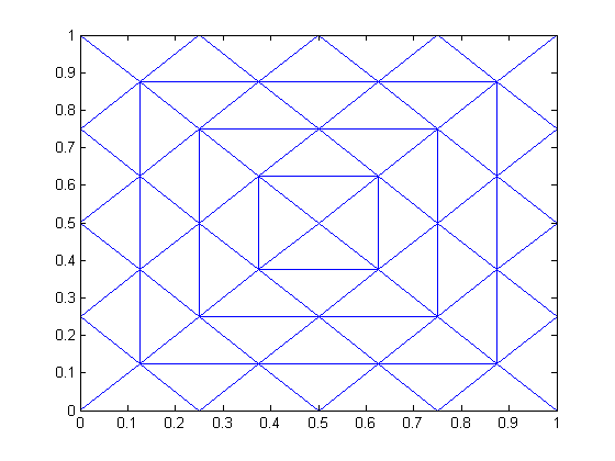
(a)

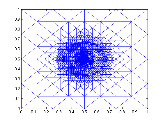
(b)

Fig. 1: (a) The initial triangulation (b) The adaptive refined mesh at the level 10.

Ndof	$\lVert u-u_{\ell}\rVert$	$\lVert{p-p}_{\ell}\rVert$	$\eta_{\ell}$	$\mu_{\ell}$	Marking Case
168	0.0571	1.3649	1.5499	4.8186	B
203	0.0435	0.9670	2.7266	4.1602	B
233	0.0336	0.8209	2.9629	3.3392	B
368	0.0254	0.6160	2.2798	2.3559	B
523	0.0197	0.4471	1.5828	1.6907	B
948	0.0152	0.3287	1.1607	1.1389	B
1783	0.0103	0.2451	0.8943	0.8198	B
3373	0.0074	0.1647	0.6013	0.5797	B
6138	0.0058	0.1334	0.4908	0.4182	A
6918	0.0048	0.1027	0.3692	0.3997	B
12053	0.0041	0.0866	0.3120	0.2941	B
21298	0.0033	0.0698	0.2527	0.2177	A
23198	0.0026	0.0547	0.1991	0.2137	B
40658	0.0022	0.0461	0.1685	0.1599	B

Table 1: Numerical results of AMFEM for Example 5.1

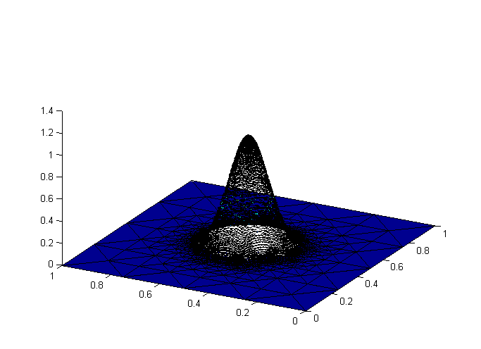
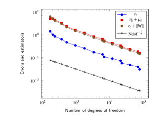
Fig. 2: Discrete solution and convergence plot

Table 5.1 displays the experimental results for errors $\lVert u-u_{\ell}\rVert$ and $\lVert{\bf p-p}_{\ell}\rVert$, the edge and volume estimators $\eta_{\ell}$ and $\mu_{\ell}$, from (10) and (11) for several consecutive levels $\ell$ of AMFEM with the number of degrees of freedom and the marking Case (A) or (B). For this example, the load function $f$ exhibits a relatively large variation in the domain and hence, within the elements. It is observed that the volume estimator $\mu_{\ell}$ is more than the edge-estimator $\eta_{\ell}$ in several levels due to large data oscillations, which results in the use of the marking Case (B) for most of the refinement levels. The reduction of $\mu_{\ell}$ influences the reduction in the edge-estimator and both lead to the optimal convergence rate ${\rm Ndof}^{-1/2}$ for errors, where Ndof denotes the number of degrees of freedom. Fig. 5.1(b) shows the adaptive refined mesh by the AMFEM algorithm at the level 10, where the number of degrees of freedom is 6918. Fig. 5.2 depicts the approximate solution $u_{h}$ and summarises the convergence rates for variables ${\bf p},u$, and sum of the estimators with respect to the number of degrees of freedom.

5.2.

For the Crack problem [2], consider the PDE (1) with coefficients $\mathbf{A}=I,~{}{\bf b}=(x-1,y+1)$ and $\gamma=4$ on$~{}\Omega=\{(x,y)\in\mathbb{R}^{2}:|{{\bf x}}|\leq 1\setminus[0,~{}1]\times\{0\}\}$ with Dirichlet boundary condition and exact solution $~{}u(r,\theta)=r^{{1}/{2}}\sin{\theta}/{2}-{r^{2}}/{2}\sin^{2}(\theta)$.

The initial uniform triangulation $\mathcal{T}_{0}$ has mesh-size $h=0.25$. The adaptive algorithm is performed with parameters $\theta_{A}=0.3,\theta_{B}=0.3$ and $\kappa=1$.

Ndof	$\lVert u-u_{\ell}\rVert$	$\lVert{p-p}_{\ell}\rVert$	$\eta_{\ell}$	$\mu_{\ell}$	Marking Case
46	0.0880	0.4021	2.0875	2.5734	A
56	0.0899	0.3979	3.4950	1.9191	B
98	0.0771	0.3557	2.3290	1.8010	B
161	0.0633	0.3085	1.3106	1.4866	A
207	0.0556	0.2643	1.1180	1.0874	B
383	0.0429	0.2401	0.6512	0.8751	A
469	0.0371	0.2042	0.5813	0.6579	A
628	0.0308	0.1695	0.4662	0.4896	A
901	0.0269	0.1400	0.3579	0.3431	B
1436	0.0207	0.1225	0.1971	0.2704	A
1821	0.0183	0.1023	0.1762	0.1949	A
2618	0.0150	0.0844	0.1433	0.1340	B
3957	0.0123	0.0746	0.0795	0.1086	A
5162	0.0111	0.0603	0.0669	0.0698	A
7482	0.0092	0.0486	0.0528	0.0453	B
12145	0.0074	0.0434	0.0282	0.0384	A
15726	0.0065	0.0351	0.0231	0.0246	A
22520	0.0054	0.0280	0.0169	0.0158	B

Table 2: Numerical results of AMFEM for Example 5.2

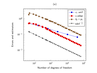
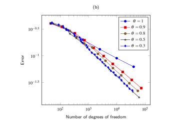
Fig. 3: (a) Convergence plots for $\theta_{A},\theta_{B}=0.3$ (b) Error convergence for $\theta=\theta_{A}=\theta_{B}$ equal to 0.3, 0.5, 0.8, 0.9, 1

Table 5.2 displays the experimental results for the errors $\lVert u-u_{\ell}\rVert$ and $\lVert{\bf p-p}_{\ell}\rVert$, the estimators $\eta_{\ell}$ and $\mu_{\ell}$ for several consecutive levels $\ell$ of AMFEM with the number of degrees of freedom and the marking Case (A) or (B) for this problem. The right-hand function $f$ of (1) in this example is not smooth and the solution has singularity at the origin, and hence the adaptive algorithm utilizes both the marking cases to achieve the optimal convergence rate. Figure 5.3(a) shows optimal convergence rate ${\rm Ndof}^{-1/2}$ for adaptive algorithm while uniform refinement yields a suboptimal convergence rate ${\rm Ndof}^{-1/4}$ for the above mentioned parameters. Figure 5.3(b) shows the convergence rate of the error for different values of $\theta_{A}$ and $\theta_{B}$. This supports the theoretical prediction of the choice of marking parameters $\theta_{A}$ and $\theta_{B}$ in the proof of Theorem 4.5, that is, the quasi-optimality can be achieved only for small values of $\theta_{A}~{}{\rm and}~{}\theta_{B}$.

5.3.

Consider the PDE (1) with coefficients $~{}\mathbf{A}=I,~{}~{}\mathbf{b}=(0,0),$  $\gamma=-8.9$, Dirichlet boundary condition on the L-shaped domain $\Omega=(-1,1)\times(-1,1)\setminus[0,1]\times[-1,0]$ and the exact solution given in polar coordinates as $u(r,\theta)=r^{2/3}\sin\big{(}2\theta/3\big{)}.$

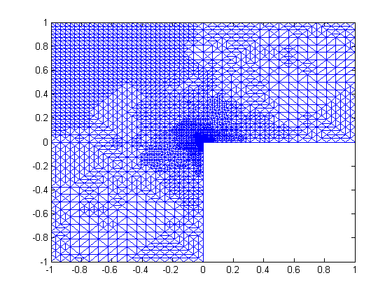
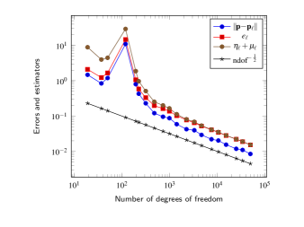
Fig. 4: Adaptive mesh-refinement and the convergence plot

The numerical experiment is performed with initial mesh-size $h=0.25$ and uniform triangulation. The adaptive algorithm is performed with parameter choice $\theta_{A}=0.5,\theta_{B}=0.5$ and $\kappa=2$. Since the forcing function $f$ is smooth, the oscillation term has higher order convergence than the remaining terms in the estimator. In this example, the marking is based on the edge estimator to obtain the optimal convergence. The refinement due to the data oscillations and the volume estimators can be avoided since they play a minor role in the convergence. Figure 5.4 displays the adaptive mesh-refinement and the optimal convergence rate ${\rm Ndof}^{-1/2}$ of the errors and the estimators for a sufficiently small mesh-size $h$.

5.4. Observations

This subsection deals with a few observations.

• If the given function $f$ has large variation in the domain and within the elements, then adaptive algorithm chooses Case (B) marking criteria and achieves the convergence (see 5.1).

• When $f$ is not smooth and the solution also has singularity, then the adaptive algorithm utilizes both the marking cases to achieve the optimal convergence rate (see 5.2).

• For the smooth function $f$, the oscillation has higher order convergence than the remaining estimator terms. In such cases, the data oscillations and the volume estimators have a very minor role in the convergence. Thus, the marking would be based on the edge-based error estimator to capture singularity of the solution (see 5.3).

6 Conclusions

In this work, the convergence and the quasi-optimality of adaptive mixed finite element method is analysed for the non-symmetric and indefinite second order elliptic equations using the lowest order Raviart-Thomas elements. The adaptive algorithm in Subsection 2.1 is designed as a combination of the edge and the volume error estimators. The numerical experiments confirm the efficiency of this algorithm and support the theoretical findings.

Acknowledgements

The first author acknowledges the financial support of Council of Scientific and Industrial Research (CSIR), Government of India. The authors sincerely thank Professor Carsten Carstensen, Humboldt University, Berlin for his constructive comments and suggestions.

References

• [1] M. Ainsworth and J. T. Oden, A posteriori error estimation in finite element analysis, Wiley, New York, 2000.
• [2] C. Bahriawati and C. Carstensen, Three matlab implementation of the lowest order Raviart-Thomas MFEM with a posteriori error control, Comput. Methods Appl. Math., 5 (2005), pp. 333-1361.
• [3] S. C. Brenner and L. R. Scott, The mathematical theory of finite element methods, third ed., Texts in Applied Mathematics, 15, Springer, New York, 2008.
• [4] R. Becker and S. Mao, An optimally convergent adaptive mixed finite element method, Numer. Math., 111 (2008), pp. 35-54.
• [5] R. Becker and S. Mao, A convergent nonconforming adaptive finite element method with quasi-optimal complexity, SIAM J. Numer. Anal., 47 (2010), pp. 4639-4659.
• [6] P. Binev, W. Dahmen, and R. DeVore, Adaptive finite element methods with convergence rates, Numer. Math., 97 (2004), pp. 219-268.
• [7] F. Brezzi and M. Fortin, Mixed and hybrid finite element methods, Springer Verlag, 1991.
• [8] C. Carstensen, A posteriori error estimate for the mixed finite element method, Math. Comp., 66 (1997), pp. 465-476.
• [9] C. Carstensen, A unifying theory of a posteriori finite element error control, Numer. Math., 100 (2005), pp. 617-637.
• [10] C. Carstensen, Convergence of adaptive finite element methods in computational mechanics, Appl. Numer. Math., 59 (2009), pp. 2119-2130.
• [11] C. Carstensen and J. Hu, A unifying theory of a posteriori error control for nonconforming finite element methods, Numer. Math., 107 (2007), pp. 473-502.
• [12] C. Carstensen, Asha. K. Dond, N. Nataraj, and Amiya. K. Pani, Error analysis of nonconforming and mixed FEMs for second-order linear non-selfadjoint and indefinite elliptic problems, http://arxiv.org/abs/1401.4810.
• [13] C. Carstensen and R. Hella, An optimal adaptive mixed finite element method, Math. Comp., 80 (2011), pp. 649-667.
• [14] C. Carstensen and R.H.W. Hoppe, Convergence analysis of adaptive nonconforming finite element methods, Numer. Math., 103 (2006), pp. 251-266.
• [15] C. Carstensen and R. H. W. Hoppe, Error reduction and convergence for an adaptive mixed finite element method, Math. Comp., 75 (2006), pp. 1033-1042.
• [16] C. Carstensen, M. Feischl, M.Page, and D. Praetorius, Axioms of Adaptivity, ASC Report 38/2013, Institute for Analysis and Scientific Computing, Vienna University of Technology.
• [17] J. Cascon, C. Kreuzer, R. H. Nochetto, and K. G. Siebert, Quasi-optimal convergence rate for an adaptive finite element method, SIAM J. Numer. Anal., 46 (2008), pp. 2524-2550.
• [18] J. Cascon, R. H. Nochetto, and K. G. Siebert, Design and convergence of AFEM in $H({\rm div})$, Math. Models Methods Appl. Sci., 17 (2007), pp. 1849-1881.
• [19] J. Chen and L. Li, Convergence and domain decomposition algorithm for nonconforming and mixed methods for nonselfadjoint and indefinite problems, Comput. Methods Appl. Engrg., 173 (1999), pp. 1-20.
• [20] L. Chen, M. Holst, and J. Xu, Convergence and optimality of adaptive mixed finite element methods, Math. Comp., 78 (2009), pp. 35-53.
• [21] H. Chen, X. Xu, and R.H.W. Hoppe, Convergence and Quasi-optimality of adaptive nonconforming finite element methods for some nonsymmetric and indefinite problems, Numer. Math., 116 (2010), pp. 383-419.
• [22] A. Demlow and R Stevenson, Convergence and quasi-optimality of an adaptive finite element method for controlling $L_{2}$ errors, Numer. Math., 117 (2011), pp. 185-218.
• [23] J. Jr. Douglas and J.E. Robert, Global estimates for mixed methods for second order elliptic equations Math. Comput. 44(1985), pp. 39-51.
• [24] M. Feischl, T. F$\ddot{u}$hrer, and D. Praetorius, Adaptive FEM with optimal convergence rates for a certain class of non-symmetric and possibly non-linear problems, ASC Report 43/2012, Institute for Analysis and Scientific Computing, Vienna University of Technology.
• [25] K. Mekchay and R.H. Nochetto, Convergence of adaptive finite element methods for general second order elliptic PDE, SIAM J. Numer. Anal., 43 (2005), pp. 1803-1827.
• [26] L. D. Marini, An inexpensive method for the evaluation of the solution of the lowest order Raviart-Thomas mixed method, SIAM J. Numer. Anal., 22 (1985), pp. 493-496.
• [27] W. D$\ddot{o}$rfler, A convergent adaptive algorithm for Poisson’s equation, SIAM J. Numer. Anal. 33 (1996), pp. 1106-1124.
• [28] P. Morin, R.H. Nochetto, and K.G. Siebert, Data oscillation and convergence of adaptive fem, SIAM J. Numer. Anal., 38 (2000), pp. 466-488.
• [29] P. Morin, R.H. Nochetto, and K.G. Siebert, Convergence of adaptive finite element methods, SIAM Rev., 44 (2002), pp. 631-658.
• [30] P. Morin, K. G. Siebert, and A. Veeser, A basic convergence result for conforming adaptive finite elements, Math. Models Methods Appl. Sci., 18 (2008), pp. 707-737.
• [31] A. H. Schatz, An observation concerning Ritz-Galerkin methods with indefinite bilinear forms, Math. Comput., 28 (1974), pp. 959-962.
• [32] A. H. Schatz and J. Wang, Some new error estimates for Ritz-Galerkin methods with minimal regularity assumptions, Math. Comp., 65 (1996), pp. 19-27.
• [33] R. Stevenson, Optimality of a standard adaptive finite element method, Found. Comput. Math., 7 (2007), pp.245-269.
• [34] R. Verfürth, A posteriori error estimation and adaptive mesh-refinement techniques, J. Comput. Appl. Math., 50 (1994), pp. 67-83.
Appendix I
List of the constants
Constant Dependency on Appears first in Value
I. Natural Constants
$C_{\rm rel}$ Coefficients of (1.1) and interpolation Positive
constants Theorem 3.2
$\epsilon$ Coefficients of (1.1) and interpolation (A posteriori Positive
constants estimates)
$h_{1}$ $\epsilon$ Positive
$C_{\rm eff}$ Coefficients of (1.1), inverse inequality Lemma 3.3 Positive
and finite overlap (efficiency)
$C_{1}$ Coefficients of (1.1) Lemma 3.4 (Volume Positive
estimator reduction)
$C_{2}$ Coefficients of (1.1), inverse inequality Lemma 3.6 (edge Positive
and finite overlap (estimator reduction)
$C_{3}$ Coefficients of (1.1) Lemma 3.7 (Quasi- Positive
orthogonality)
$C_{4}$ Coefficients of (1.1), Lemma 3.9 Positive
interpolation constants (Quasi-reliability)
$\gamma_{0}$ $\left\{\begin{array}[]{l l}0<\gamma_{0}<1&~{}~{}\text{if $T\in\mathcal{T}_{H},$ refined}\\ 1&\quad\text{otherwise}\end{array}\right.$ Corollary 3.5 Positive
II. Contraction property
$\theta_{B}$ $0<\theta_{B}<1$, to be chosen (0,1)
$\delta_{1}$ $<\frac{\theta_{B}}{4-\theta_{B}}$ Lemma 3.4 (0,1)
$\rho_{B}$ $(1+\delta_{1})(1-\frac{\theta_{B}}{4})$ (volume-estimator (0,1)
$\varLambda_{1}$ $C_{1}(1+\frac{1}{\delta_{1}})$ reduction ) (0,1)
$\theta_{A}$ $0<\theta_{A}<1$, to be chosen (0,1)
$\delta_{2}$ $\frac{\theta_{A}}{4-2\theta_{A}}$ Lemma 3.6 (0,1)
$\varLambda_{2}$ $C_{2}(1+\frac{1}{\delta_{2}})$ (edge-estimator (0,1)
$\rho_{A}$ $(1+\frac{1}{\delta_{2}})(1-\frac{\theta_{A}}{2})$ reduction ) (0,1)
$C_{3}$ Coefficient of (1.1) Positive
$\alpha_{2}$ $0.5+7C_{3}^{2}\varLambda_{1}H^{2}$ Lemma 3.6 (0,1)
$\alpha_{3}$ $0.5-7C_{3}^{2}\varLambda_{1}H^{2}$ (Quasi- (0,1)
$\delta_{3}$ $<$1 orthogonality) (0,1)
$\alpha_{1}$ $\delta_{3}+4C_{3}^{2}\epsilon^{2}$ (0,1)
$\alpha_{4}$ $\frac{1}{2}\min\{1,\frac{(1-\rho_{A})\alpha_{3}}{({\varLambda_{1}+\varLambda_{2}})C_{\rm rel}}\}$ (0,1)
$\delta_{3}$ $<\alpha_{4}$ Remark 3.2 (0,1)
$\epsilon$ $(\alpha_{4}-\delta_{3})/(4C_{3}^{2})$ Positive
$h_{2}$ $\epsilon~{}{\rm and}~{}<\frac{1}{\sqrt{14C_{3}^{2}\varLambda_{1}}}$ Positive
$\alpha_{1}$ $<\alpha_{4}$ (0,1)
$C_{5}$ $({\varLambda_{1}+\varLambda_{2}})/{\alpha_{3}}$ Positive
$\alpha$ $C_{5}(1-\alpha_{1})$ Positive
$h_{3}$ $\min\{h_{1},h_{2},\frac{1}{\sqrt{\beta}}\}$ Positive
$E$ $2(C_{5}\varLambda_{3}+C_{5}\alpha_{4}C_{rel})$ Theorem 4.1 Positive