A High-Performance Triple Patterning Layout Decomposer
with Balanced Density

Abstract

Triple patterning lithography (TPL) has received more and more attentions from industry as one of the leading candidate for 14nm/11nm nodes. In this paper, we propose a high performance layout decomposer for TPL. Density balancing is seamlessly integrated into all key steps in our TPL layout decomposition, including density-balanced semi-definite programming (SDP), density-based mapping, and density-balanced graph simplification. Our new TPL decomposer can obtain high performance even compared to previous state-of-the-art layout decomposers which are not balanced-density aware, e.g., by Yu et al. (ICCAD’11), Fang et al. (DAC’12), and Kuang et al. (DAC’13). Furthermore, the balanced-density version of our decomposer can provide more balanced density which leads to less edge placement error (EPE), while the conflict and stitch numbers are still very comparable to our non-balanced-density baseline.

I Introduction

As the minimum feature size further decreases, the semiconductor industry faces great challenge in patterning sub-22nm half-pitch due to the delay of viable next generation lithography, such as extreme ultra violet (EUV) and electric beam lithography (EBL). Triple patterning lithography (TPL), along with self-aligned double patterning (SADP), are solution candidates for the 14nm logic node [1]. Both TPL and SADP are similar to double patterning lithography (DPL), but with different or more exposure/etching processes [2]. SADP may be significantly restrictive on design, i.e., cannot handle irregular arrangements of contacts and does not allow stitching. Therefore, TPL began to receive more attention from industry, especially for metal 1 layer patterns. For example, industry has already explored test-chip patterns with triple patterning and even quadruple patterning [3].

Similar to DPL, the key challenge of TPL lies in the decomposition process where the original layout is divided into three masks. During decomposition, when the distance between any two features is less than the minimum coloring distance $dis_{m}$, they need to be assigned into different masks to avoid a conflict. Sometimes, a conflict can be resolved by splitting a pattern into two touching parts, called stitches. After the TPL layout decomposition, the features are assigned into three masks (colors) to remove all conflicts. The advantage of TPL is that the effective pitch can be tripled which can further improve lithography resolution. Besides, some native conflicts in DPL can be resolved.

In layout decomposition, especially for TPL, density balance should also be considered, along with the conflict and stitch minimization. A good pattern density balance is also expected to be a consideration in mask CD and registration control [4], while unbalanced density would cause lithography hotspots as well as lowered CD uniformity due to irregular pitches [5]. However, from the algorithmic perspective, achieving a balanced density in TPL could be harder than that in DPL. (1) In DPL, two colors can be more implicitly balanced; while in TPL, often times existing/previous strategies may try to do DPL first, and then do some “patch” with the third mask, which causes a big challenge to “explicitly” consider the density balance. (2) Due to the one more color, the solution space is much larger [6]. (3) Instead of global density balance, local density balance should be considered to reduce the potential hotspots, since neighboring patterns are one of the main sources of hotspots. As shown in Fig. 1 (a)(b), when only global density balance is considered, feature $a$ is assigned white color. Since two black features are close to each other, hotspot may be introduced. To consider the local density balance, the layout is partitioned into four bins {$b_{1},b_{2},b_{3},b_{4}$} (see Fig. 1 (c)). Feature $a$ is covered by bins $b_{1}$ and $b_{2}$, therefore it is colored as blue to maintain the local density balances for both bins (see Fig. 1 (d)).

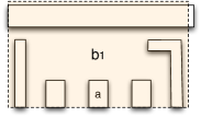
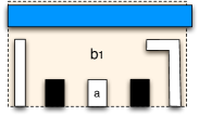
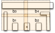
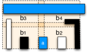
Figure 1:  Decomposed layout with (a) (b) global balanced density. (c) (d) local balanced density in all bins.

There are investigations on TPL layout decomposition [6, 7, 8, 9, 10, 11] or TPL aware design [12, 13, 14]. [6] provided a three coloring algorithm, which adopts a SAT Solver. Yu et al. [7] proposed a systematic study for the TPL layout decomposition, where they showed that this problem is NP-hard. Fang et al. [8] presented several graph simplification techniques to reduce the problem size, and a maximum independent set (MIS) based heuristic for the layout decomposition. [9] proposed a layout decomposer for row structure layout. However, these existing studies suffer from one or more of the following issues: (1) cannot integrate the stitch minimization for the general layout, or can only deal with stitch minimization as a post-process; (2) directly extend the methodologies from DPL, which loses the global view for TPL; (3) assigning colors one by one prohibits the ability for density balance.

In this paper, we propose a high performance layout decomposer for TPL. Compared with previous works, our decomposer provides not only less conflict and stitch number, but also more balanced density. In this work, we focus on the coloring algorithms and leave other layout related optimizations to post-coloring stages, such as compensation for various mask overlay errors introduced by scanner and mask write control processes. However, we do explicitly consider balancing density during coloring, since it is known that mask write overlay control generally benefits from improved density balance.

Our key contributions include the following. (1) Accurately integrate density balance into the mathematical formulation; (2) Develop a three-way partition based mapping, which not only achieves less conflicts, but also more balanced density; (3) Propose several techniques to speedup the layout decomposition; (4) Our experiments show the best results in solution quality while maintaining better balanced density (i.e., less EPE).

The rest of the paper is organized as follows. Section II presents the basic concepts and the problem formulation. Section III gives the overall decomposition flow. Section IV presents the details to improve balance density and decomposition performance, and Section V shows how we further speedup our decomposer. Section VI presents our experimental results, followed by a conclusion in Section VII.

II Problem Formulation

Given input layout which is specified by features in polygonal shapes, we partition the layout into $n$ bins $B=\{b_{1},\dots,b_{n}\}$. Note that neighboring bins may share some overlapping. For each polygonal feature $r_{i}$, we denote its area as $den_{i}$, and its area covered by bin $b_{k}$ as $den_{ki}$. Clearly $den_{i}\geq den_{ki}$ for any bin $b_{k}$. During layout decomposition, all polygonal features are divided into three masks. For each bin $b_{k}$, we define three densities ($d_{k1},d_{k2},d_{k3}$), where $d_{kc}=\sum den_{ki}$, for any feature $r_{i}$ assigned to color $c$. Therefore, we can define the local density uniformity as follows:

Definition 1 (Local Density Uniformity).

For the bin $b_{k}$ $\in S$, the local density uniformity is $\textrm{max}\{d_{kc}\}/\textrm{min}\{d_{kc}\}$ given three densities $d_{k1},d_{k2}$ and $d_{k3}$ for three masks and is used to measure the ratio difference of the densities. A lower value means better local density balance. The local density uniformity is denoted by $DU_{k}$.

For convenience, we use the term density uniformity to refer to local density uniformity in the rest of this paper. It is easy to see that $DU_{k}$ is always larger than or equal to 1. To keep a more balanced density in bin $b_{k}$, we expect $DU_{k}$ as small as possible, i.e., close to 1.

Problem 1 (Density Balanced Layout Decomposition).

Given a layout which is specified by features in polygonal shapes, the layout graphs and the decomposition graphs are constructed. Our goal is to assign all vertices in the decomposition graph into three colors (masks) to minimize the stitch number and the conflict number, while keeping all density uniformities $DU_{k}$ as small as possible.

III Overall Decomposition Flow

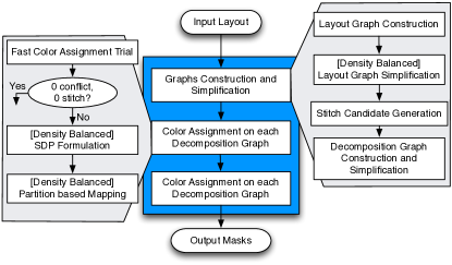
Figure 2:  Overall flow of proposed density balanced decomposer.

The overall flow of our TPL decomposer is illustrated in Fig. 2. It consists of two stages: graph construction / simplification, and color assignment. Given input layout, layout graphs and decomposition graphs are constructed, then graph simplifications [7][8] are applied to reduce the problem size. Two additional graph simplification techniques are introduced in Sec. V-A and V-B. During stitch candidate generation, the methods described in [11] are applied to search all stitch candidates for TPL. In second stage, for each decomposition graph, color assignment is proposed to assign each vertex one color. Before calling SDP formulation, fast color assignment trial is proposed to achieve better speedup (see Section V-C).

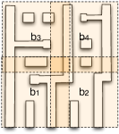
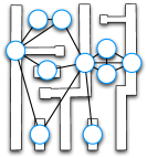
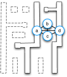
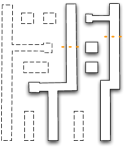
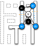
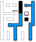
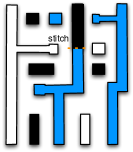
Figure 3:  An example of the layout decomposition flow.

Fig. 3 illustrates an example to show the decomposition process step by step. Given the input layout as in Fig. 3(a), we partition it into a set of bins $\{b_{1},b_{2},b_{3},b_{4}\}$ (see Fig. 3(b)). Then the layout graph is constructed (see Fig. 3(c)), where the ten vertices representing the ten features in the input layout, and each vertex represents a polygonal feature (shape) where there is an edge (conflict edge) between two vertices if and only if those two vertices are within the minimum coloring distance $min_{s}$. During the layout graph simplification, the vertices whose degree equal or smaller than two are iteratively removed from the graph. The simplified layout graph, shown in Fig. 3(d), only contains vertices $a,b,c$ and $d$. Fig. 3(d) shows the projection results. Followed by stitch candidate generation [11], there are two stitch candidates for TPL (see Fig. 3(e)). Based on the two stitch candidates, vertices $a$ and $d$ are divided into two vertices, respectively. The constructed decomposition graph is given in Fig. 3(f). It maintains all the information about conflict edges and stitch candidates, where the solid edges are the conflict edges while the dashed edges are the stitch edges and function as stitch candidates. In each decomposition graph, a color assignment, which contains semidefinite programming (SDP) formulation and partition based mapping, is carried out. During color assignment, the six vertices in the decomposition graph are assigned into three groups: $\{a_{1},c\},\{b\}$ and $\{a_{2},d_{1},d_{2}\}$ (see Fig. 3(g) and Fig. 3(h)). Here one stitch on feature $a$ is introduced. After iteratively recover the removed vertices, the final decomposed layout is shown in Fig. 3(i). Our last process should be decomposition graphs merging, which combines the results on all decomposition graphs. Since this example has only one decomposition graph, this process is skipped.

IV Density Balanced Decomposition

Density balance, especially local density balance, is seamlessly integrated into each step of our decomposition flow. In this section, we first elaborate how to integrate the density balance into the mathematical formulation and corresponding SDP formulation. Followed by some discussion for density balance in all other steps.

IV-A Density Balanced SDP Algorithm

TABLE I: Notations used in color assignment

$CE$	the set of conflict edges
$SE$	the set of stitch edges
$V$	the set of features
$B$	the set of local bins

For each decomposition graph, density balanced color assignment is carried out. Some notations used are listed in Table I. See Appendix for some preliminary of semidefinite programming (SDP) based algorithm.

IV-A1 Density Balanced Mathematical Formulation

The mathematical formulation for the general density balanced layout decomposition is shown in (1), where the objective is to simultaneously minimize the conflict number, the stitch number and the density uniformity of all bins. Here $\alpha$ and $\beta$ are user-defined parameters for assigning the relative weights among the three values.

min $$\sum_{e_{ij}\in CE}c_{ij}+\alpha\sum_{e_{ij}\in SE}s_{ij}+\beta\cdot\sum_{b_{k}\in B}DU_{k}$$ (1)

$$\textrm{s.t}.\ \ c_{ij}=(x_{i}==x_{j})\qquad\qquad\qquad\ \forall e_{ij}\in CE 1a$$ ()

$$s_{ij}=x_{i}\oplus x_{j}\qquad\qquad\qquad\qquad\forall e_{ij}\in SE 1b$$ ()

$$x_{i}\in\{1,2,3\}\qquad\qquad\qquad\qquad\forall r_{i}\in V 1c$$ ()

$$d_{kc}=\sum_{x_{i}=c}den_{ki}\quad\qquad\qquad\forall r_{i}\in V,\ \ b_{k}\in B 1d$$ ()

$$DU_{k}=\textrm{max}\{d_{kc}\}/\textrm{min}\{d_{kc}\}\qquad\forall b_{k}\in B 1e$$ ()

Here $x_{i}$ is a variable representing the color (mask) of feature $r_{i}$, $c_{ij}$ is a binary variable for the conflict edge $e_{ij}\in CE$, and $s_{ij}$ is a binary variable for the stitch edge $e_{ij}\in SE$. The constraints ($1a$) and ($1b$) are used to evaluate the conflict number and stitch number, respectively. The constraint ($1e$) is nonlinear, which makes the program (1) hard to be formulated into integer linear programming (ILP) as in [7]. Similar nonlinear constraints occur in the floorplanning problem [15], where Tayor expansion is used to linearize the constraint into ILP. However, Tayor expansion will introduce the penalty of accuracy. Compared with the traditional time consuming ILP, semidefinite programming (SDP) has been shown to be a better approach in terms of runtime and solution quality tradeoffs [7]. However, how to integrate the density balance into the SDP formulation is still an open question. In the following we will show that instead of using the painful Tayor expansion, this nonlinear constraint can be integrated into SDP without losing any accuracy.

IV-A2 Density Balanced SDP Formulation

In SDP formulation, the objective function is the representation of vector inner products, i.e., $\vec{v_{i}}\cdot\vec{v_{j}}$. At the first glance, the constraint ($1e$) cannot be formulated into an inner product format. However, we will show that density uniformity $DU_{k}$ can be optimized through considering another form $DU_{k}^{*}=d_{k1}\cdot d_{k2}+d_{k1}\cdot d_{k3}+d_{k2}\cdot d_{k3}$. This is based on the following observation: maximizing $DU_{k}^{*}$ is equivalent to minimizing $DU_{k}$.

Lemma 1.

$DU_{k}^{*}=2/3\cdot\sum_{i,j\in V}den_{ki}\cdot den_{kj}\cdot(1-\vec{v_{i}}\cdot\vec{v_{j}})$, where $den_{ki}$ is the density of feature $r_{i}$ in bin $b_{k}$.

Proof.

First of all, let us calculate $d_{1}\cdot d_{2}$. For all vectors $\vec{v_{i}}=(1,0)$ and all vectors $\vec{v_{j}}=(-\frac{1}{2},\frac{\sqrt{3}}{2})$, we can see that

$$\sum_{i}\sum_{j}len_{i}\cdot len_{j}\cdot(1-\vec{v_{i}}\cdot\vec{v_{j}})=\sum_{i}\sum_{j}len_{i}\cdot len_{j}\cdot 3/2$$

$$= 3/2\cdot\sum_{i}len_{i}\sum_{j}len_{j}=3/2\cdot d_{1}\cdot d_{2}$$

So $d_{1}\cdot d_{2}=2/3\cdot\sum_{i}\sum_{j}len_{i}\cdot len_{j}\cdot(1-\vec{v_{i}}\cdot\vec{v_{j}})$, where $\vec{v_{i}}=(1,0)$ and $\vec{v_{j}}=(-\frac{1}{2},\frac{\sqrt{3}}{2})$. We can also calculate $d_{1}\cdot d_{3}$ and $d_{2}\cdot d_{3}$ using similar methods. Therefore,

$$DU_{2} =d_{1}\cdot d_{2}+d_{1}\cdot d_{3}+d_{2}\cdot d_{3}$$

$$=2/3\cdot\sum_{i,j\in V}len_{i}\cdot len_{j}\cdot(1-\vec{v_{i}}\cdot\vec{v_{j}})$$

Because of Lemma 1, the $DU_{k}^{*}$ can be represented as a vector inner product, then we have achieved the following theorem.

Theorem 1.

Maximizing $DU_{k}^{*}$ can achieve better density balance in bin $b_{k}$.

Note that we can remove the constant $\sum_{i,j\in V}den_{ki}\cdot den_{kj}\cdot 1$ in $DU_{k}^{*}$ expression. Similarly, we can eliminate the constants in the calculation of the conflict and stitch numbers. The simplified vector program is as follows:

min $$\sum_{e_{ij}\in CE}(\vec{v_{i}}\cdot\vec{v_{j}})-\alpha\sum_{e_{ij}\in SE}(\vec{v_{i}}\cdot\vec{v_{j}})-\beta\cdot\sum_{b_{k}\in B}DU_{k}^{*}$$ (2)

$$\textrm{s.t}.\ \ DU_{k}^{*}=-\sum_{i,j\in V}den_{ki}\cdot den_{kj}\cdot(\vec{v_{i}}\cdot\vec{v_{j}})\quad\forall b_{k}\in B 2a$$ ()

$$\vec{v_{i}}\in\{(1,0),(-\frac{1}{2},\frac{\sqrt{3}}{2}),(-\frac{1}{2},-\frac{\sqrt{3}}{2})\} 2b$$ ()

Formulation (2) is equivalent to the mathematical formulation (1), and it is still NP-hard to be solved exactly. Constraint ($2b$) requires the solutions to be discrete. To achieve a good tradeoff between runtime and accuracy, we can relax (2) into a SDP formulation, as shown in Theorem 2.

Theorem 2.

Relaxing vector program (2) can get the SDP formulation (3).

SDP:  min $$\ \ \ A\bullet X$$ (3)

$$X_{ii}=1,\ \ \forall i\in V 3a$$ ()

$$X_{ij}\geq-\frac{1}{2},\ \ \forall e_{ij}\in CE 3b$$ ()

$$X\succeq 0 3c$$ ()

where $A_{ij}$ is the entry that lies in the $i$-th row and the $j$-th column of matrix $A$:

$$A_{ij}=\left\{\begin{array}[]{cc}1+\beta\cdot\sum_{k}den_{ki}\cdot den_{kj},&\forall b_{k}\in B,e_{ij}\in CE\\ -\alpha+\beta\cdot\sum_{k}den_{ki}\cdot den_{kj},&\forall b_{k}\in B,e_{ij}\in SE\\ \beta\cdot\sum_{k}den_{ki}\cdot den_{kj},&\textrm{otherwise}\end{array}\right.$$

Due to space limit, the detailed proof is omitted. The solution of (3) is continuous instead of discrete, and provides a lower bound of vector program (2). In other words, (3) provides an approximated solution to (2).

IV-B Density Balanced Mapping

Each $X_{ij}$ in solution of (3) corresponds to a feature pair $(r_{i},r_{j})$. The value of $X_{ij}$ provides a guideline, i.e., whether two features $r_{i}$ and $r_{j}$ should be in same color. If $X_{ij}$ is close to $1$, features $r_{i}$ and $r_{j}$ tend to be in the same color (mask); while if it is close to $-0.5$, $r_{i}$ and $r_{j}$ tend to be in different colors (masks). With these guidelines a mapping procedure is adopted to finally assign all input features into three colors (masks).

IV-B1 Limitations of Greedy Mapping

In [7], a greedy approach was applied for the final color assignment. The idea is straightforward: all $X_{ij}$ values are sorted, and vertices $r_{i}$ and $r_{j}$ with larger $X_{ij}$ value tend to be in the same color. The $X_{ij}$ can be classified into two types: clear and vague. If most of the $X_{ij}$s in matrix $X$ are clear (close to 1 or -0.5), this greedy method may achieve good result. However, if the decomposition graph is not 3-colorable, some values in matrix $X$ are vague. For the vague $X_{ij}$, e.g., 0.5, the greedy method may not be so effective.

IV-B2 Density Balanced Partition based Mapping

Contrary to the previous greedy approach, we propose a partition based mapping, which can solve the assignment problem for the vague $X_{ij}$s in a more effective way. The new mapping is based on a three-way maximum-cut partitioning. The main ideas are as follows. If a $X_{ij}$ is vague, instead of only relying on the SDP solution, we also take advantage of the information in decomposition graph. The information is captured through constructing a graph, denoted by $G_{M}$. Through formulating the mapping as a three-way partitioning on the graph $G_{M}$, our mapping can provide a global view to search better solutions.

Algorithm 1 Partition based Mapping

0:  Solution matrix $X$ of the program (3).

1:  Label each non-zero entry $X_{i,j}$ as a triplet $(X_{ij},i,j)$;

2:  Sort all $(X_{ij},i,j)$ by $X_{ij}$;

3:  for  all triples with $X_{ij}>th_{unn}$ do

4:     Union(i, j);

5:  end for

6:  for  all triples with $X_{ij}<th_{sp}$ do

7:     Separate(i, j);

8:  end for

9:  Construct graph $G_{M}$;

10:  if graph size $\leq$ 3 then

11:     return;

12:  else if graph size $\leq 7$ then

13:     Backtracking based three-way partitioning;

14:  else

15:     FM based three-way partitioning;

16:  end if

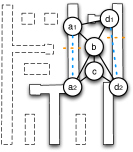
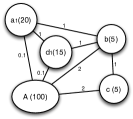
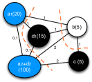
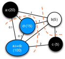
Figure 4: Density Balanced Mapping.  (a) Decomposition graph. (b) Construct graph $G_{M}$.  (c) Mapping result with cut value 8.1 and density uniformities 24.  (d) A better mapping with cut 8.1 and density uniformities 23.

Algorithm 1 shows our partition based mapping procedure. Given the solutions from program (3), some triplets are constructed and sorted to maintain all non-zero $X_{ij}$ values (lines 1–2). The mapping incorporates two stages to deal with the two different types. The first stage (lines 3–8) is similar to that in [7]. If $X_{ij}$ is clear then the relationship between vertices $r_{i}$ and $r_{j}$ can be directly determined. Here $th_{unn}$ and $th_{sp}$ are user-defined threshold values. For example, if $X_{ij}>th_{unn}$, which means that $r_{i}$ and $r_{j}$ should be in the same color, then function Union(i, j) is applied to merge them into a large vertex. Similarly, if $X_{ij}<th_{sp}$, then function Separate(i, j) is used to label $r_{i}$ and $r_{j}$ as incompatible. In the second stage (lines 9–16) we deal with the vague $X_{ij}$ values. During the previous stage some vertices have been merged, therefore the total vertex number is not large. Here we construct a graph $G_{M}$ to represent the relationships among all the remanent vertices (line 9). Each edge $e_{ij}$ in this graph has a weight representing the cost if vertices $i$ and $j$ are assigned into same color. Therefore, the color assignment problem can be formulated as a maximum-cut partitioning problem on $G_{M}$ (line 10–16).

Through assigning a weight to each vertex representing its density, graph $G_{M}$ is able to balance density among different bins. Based on the $G_{M}$, a partitioning is performed to simultaneously achieve a maximum-cut and balanced weight among different parts. Note that we need to modify the gain function, then in each move, we try to achieve a more balanced and larger cut partitions.

An example of the density balanced mapping is shown in Fig. 4. Based on the decomposition graph (see Fig. 4 (a)), SDP is formulated. Given the solutions of SDP, after the first stage of mapping, vertices $a_{2}$ and $d_{2}$ are merged in to a large vertex. As shown in Fig. 4(b), the graph $G_{M}$ is constructed, where each vertex is associated with a weight. There are two partition results with the same cut value 8.1 (see Fig. 4 (c) and Fig. 4 (d)). However, their density uniformities are 24 and 23, respectively. To keep a more balanced density result, the second partitioning in Fig. 4 (c) is adopted as color assignment result.

It is well known that the maximum-cut problem, even for a 2-way partition, is NP-hard. However, we observe that in many cases, after the global SDP optimization, the graph size of $G_{M}$ could be quite small, i.e., less than 7. For these small cases, we develop a backtracking based method to search the entire solution space. Note that here backtracking can quickly find the optimal solution even through three-way partitioning is NP-hard. If the graph size is larger, we propose a heuristic method, motivated by the classic FM partitioning algorithm [16][17]. Different from the classic FM algorithm, we make the following modifications. (1) In the first stage of mapping, some vertices are labeled as incomparable, therefore before moving a vertex from one partition to another, we should check whether it is legal. (2) Classical FM algorithm is for min-cut problem, we need to modify the gain function of each move to achieve a maximum cut.

The runtime complexity of graph construction is $O(m)$, where $m$ is the vertex number in $G_{M}$. The runtime of three-way maximum-cut partitioning algorithm is $O(mlogm)$. Besides, the first stage of mapping needs $O(n^{2}logn)$ [7]. Since $m$ is much smaller than $n$, the complexity of density balanced mapping is $O(n^{2}logn)$.

IV-C Density Balanced Layout Graph Simplification

Here we show that the layout graph simplification, which was proposed in [7], can consider the local density balance as well. During layout graph simplification, we iteratively remove and push all vertices with degree less than or equal to two. After the color assignment on the remained vertices, we iteratively recover all the removed vertices and assign legal colors. Instead of randomly picking one, we search a legal color which is good for the density uniformities.

V Speedup Techniques

Our layout decomposer applies a set of graph simplification techniques proposed by recent works:

• Independent Component Computation [7][8][11];

• Vertex with Degree Less than 3 Removal [7][8][11];

• 2-Edge-Connected Component Computation [7][8][11];

• 2-Vertex-Connected Component Computation [8][11].

Apart from the above graph simplifications, our decomposer proposes a set of novel speedup techniques, which would be introduced in this section.

V-A LG Cut Vertex Stitch Forbiddance

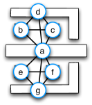
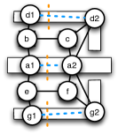
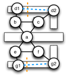
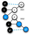
Figure 5: Layout graph cut vertex stitch forbiddance.

A vertex of a graph is called a cut vertex if its removal decomposes the graph into two or more connected components. Cut vertices can be identified through the process of bridge computation [7]. During stitch candidate generation, forbidding any stitch candidate on cut vertices can be helpful for later decomposition graph simplification. Fig. 5 (a) shows a layout graph, where feature $a$ is a cut vertex, since its removal can partition the layout graph into two parts: {b, c, d} and {e, f, g}. If stitch candidates are introduced within $a$, the corresponding decomposition graph is illustrated in Fig. 5 (b), which is hard to be further simplified. If we forbid the stitch candidate on $a$, the corresponding decomposition graph is shown in Fig. 5 (c), where $a$ is still cut vertex in decomposition graph. Therefore we can apply 2-connected component computation [8] to simplify the problem size, and apply color assignment separately (see Fig. 5 (d)).

V-B Decomposition Graph Vertex Clustering

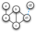
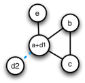
Figure 6: DG vertex clustering to reduce the decomposition graph size.

Decomposition graph vertex clustering is a speedup technique to further reduce the decomposition graph size. As shown in Fig. 6 (a), vertices $a$ and $d_{1}$ share the same conflict relationships against $b$ and $c$. Besides, there is no conflict edges between $a$ and $d_{1}$. If no conflict is introduced, vertices $a$ and $d_{1}$ should be assigned the same color, therefore we can cluster them together, as shown in Fig. 6 (b). Note that the stitch and conflict relationships are also merged. Applying vertex clustering in decomposition graph can further reduce the problem size.

V-C Fast Color Assignment Trial

Although the SDP and the partition based mapping can provide high performance for color assignment, it is still expensive to be applied to all the decomposition graphs. We derive a fast color assignment trial before calling SDP based method. If no conflict or stitch is introduced, our trial solves the color assignment problem in linear time. Note that SDP method is skipped only when decomposition graph can be colored without stitch or conflict, our fast trial does not lose any solution quality. Besides, our preliminary results show that more than half of the decomposition graphs can be decomposed using this fast method. Therefore, the runtime can be dramatically reduced.

Algorithm 2 Fast Color Assignment Trial

0:  Decomposition graph $G$, stack $S$.

1:  while $\exists n\in G$ s.t. $d_{conf}(n)<3$ & $d_{stit}(n)<2$ do

2:     $S.push(n)$; $G.delete(n)$;

3:  end while

4:  if $G$ is not empty then

5:     Recover all vertices in $S$;

6:     return  false;

7:  else

8:     while  $!S.empty()$ do

9:        $n=S.pop()$; $G.add(n)$;

10:        Assign $n$ a legal color;

11:     end while

12:     return  true;

13:  end if

The fast color assignment trial is shown in Algorithm 2. First, we iteratively remove the vertex with conflict degree ($d_{conf}$) less than 3 and stitch degree ($d_{stit}$) less than 2 (lines 1–3). If some vertices cannot be removed, we recover all the vertices in stack $S$, then return $false$; Otherwise, the vertices in $S$ are iteratively popped (recovered) (lines 8–12). For each vertex $n$ popped, since it is connected with at most one stitch edge, we can always assign one color without introducing conflict or stitch.

TABLE II: Comparison of Runtime and Performance.

Circuit	ICCAD’11 [7]				DAC’12 [8]				DAC’13 [11]				SDP+PM
	cn#	st#	cost	CPU(s)	cn#	st#	cost	CPU(s)	cn#	st#	cost	CPU(s)	cn#	st#	cost	CPU(s)
C432	3	1	3.1	0.09	0	6	0.6	0.03	0	4	0.4	0.01	0	4	0.4	0.2
C499	0	0	0	0.07	0	0	0	0.04	0	0	0	0.01	0	0	0	0.2
C880	1	6	1.6	0.15	1	15	2.5	0.05	0	7	0.7	0.01	0	7	0.7	0.3
C1355	1	2	1.2	0.07	1	7	1.7	0.07	0	3	0.3	0.01	0	3	0.3	0.3
C1908	0	1	0.1	0.07	1	0	1	0.1	0	1	0.1	0.01	0	1	0.1	0.3
C2670	2	4	2.4	0.17	2	14	3.4	0.16	0	6	0.6	0.04	0	6	0.6	0.4
C3540	5	6	5.6	0.27	2	15	3.5	0.2	1	8	1.8	0.05	1	8	1.8	0.5
C5315	7	7	7.7	0.3	3	11	4.1	0.27	0	9	0.9	0.05	0	9	0.9	0.7
C6288	82	131	95.1	3.81	19	341	53.1	0.3	14	191	33.1	0.25	1	213	22.3	2.7
C7552	12	15	13.5	0.77	3	46	7.6	0.42	1	21	3.1	0.1	0	22	2.2	1.1
S1488	1	1	1.1	0.16	0	4	0.4	0.08	0	2	0.2	0.01	0	2	0.2	0.3
S38417	44	55	49.5	18.8	20	122	32.2	1.25	19	55	24.5	0.42	19	55	24.5	7.9
S35932	93	18	94.8	89.7	46	103	56.3	4.3	44	41	48.1	0.82	44	48	48.8	21.4
S38584	63	122	75.2	92.1	36	280	38.8	3.7	36	116	47.6	0.77	37	118	48.8	22.2
S15850	73	91	82.1	79.8	36	201	56.1	3.7	36	97	45.7	0.76	34	101	44.1	20.0
avg.	25.8	30.7	28.9	19.1	11.3	60.87	17.42	0.978	10.1	37.4	13.8	0.22	9.07	39.8	13.0	5.23
ratio			2.2	3.65			1.34	0.19			1.06	0.04			1.0	1.0

TABLE III: Comparison on Very Dense Layouts

Circuit	ICCAD 2011 [7]				DAC 2012 [8]				SDP+PM
	cn#	st#	cost	CPU(s)	cn#	st#	cost	CPU(s)	cn#	st#	cost	CPU(s)
mul_top	836	44	840.4	236	457	0	457	0.8	118	271	145.1	57.6
exu_ecc	119	1	119.1	11.1	53	0	53	0.7	22	64	28.4	4.3
c9_total	886	228	908.8	47.4	603	641	667.1	0.52	117	1009	217.9	7.7
c10_total	2088	554	2143.4	52	1756	1776	1933.6	1.1	248	1876	435.6	19
s2_total	2182	390	2221	936.8	1652	5976	2249.6	4	703	5226	1225.6	70.7
s3_total	6844	72	6851.2	7510.1	4731	13853	6116.3	13.1	958	10572	2015.2	254.5
s4_total	NA	NA	NA	$>$10000	3868	13632	5231.2	13	1151	11091	2260.1	306
s5_total	NA	NA	NA	$>$10000	4650	16152	6265.2	12.9	1391	13683	2759.3	350.4
avg.	NA	NA	NA	$>$3600	2221.3	6503.8	2871.6	5.8	588.5	5474	1135.9	134
ratio			-	$>$27.0			2.53	0.05			1.0	1.0

VI Experimental Results

We implement our decomposer in C++ and test it on an Intel Xeon 3.0GHz Linux machine with 32G RAM. ISCAS 85&89 benchmarks from [7] are used, where the minimum coloring spacing $dis_{m}$ was set the same with previous studies [7][8]. Besides, to perform a comprehensive comparison, we also test on other two benchmark suites. The first suite is with six dense benchmarks (“c9_total”-“s5_total”), while the second suite is two synthesized OpenSPARC T1 designs “mul_top” and “exu_ecc” with Nangate 45nm standard cell library [18]. When processing these two benchmark suites we set the minimum coloring distance $dis_{m}=2\cdot w_{min}+3\cdot s_{min}$, where $w_{min}$ and $s_{min}$ denote the minimum wire width and the minimum spacing, respectively. The parameter $\alpha$ is set as $0.1$. The size of each bin is set as $10\cdot dis_{m}\times 10\cdot dis_{m}$. We use CSDP [19] as the solver for the semidefinite programming (SDP).

VI-A Comparison with other decomposers

In the first experiment, we compare our decomposer with the state-of-the-art layout decomposers which are not balanced density aware [7][8][11]. We obtain the binary files from [7] and [8]. Since currently we cannot obtain the binary for decomposer in [11], we directly use the results listed in [11]. Here our decomposer is denoted as “SDP+PM”, where “PM” means the partition based mapping. The $\beta$ is set as 0. In other words, SDP+PM only optimizes for stitch and conflict number. Table III shows the comparison in terms of runtime and performance. For each decomposer we list its stitch number, conflict number, cost and runtime. The columns “cn#” and “st#” denote the conflict number and the stitch number, respectively. “cost” is the cost function, which is set as cn# $+0.1\times$ st#. “CPU(s)” is computational time in seconds.

First, we compare SDP+PM with the decomposer in [7], which is based on SDP formulation as well. From Table III we can see that the new stitch candidate generation (see [11] for more details) and partition-based mapping can achieve better performance (reducing the cost by around 55%). Besides, SDP+PM can get nearly $4\times$ speed-up. The reason is that, compared with [7], a set of speedup techniques, i.e., 2-vertex-connected component computation, layout graph cut vertex stitch forbiddance (Sec. V-A), decomposition graph vertex clustering (Sec. V-B), and fast color assignment trial (Sec. V-C), are proposed. Second, we compare SDP+PM with the decomposer in [8], which applies several graph based simplifications and maximum independent set (MIS) based heuristic. From Table III we can see that although the decomposer in [8] is faster, MIS based heuristic has worse solution qualities (around 33% cost penalty compared to SDP+PM). Compared with the decomposer in [11], although SDP+PM is slower, it can reduce the cost by around 6%.

In addition, we compare SDP-PM with other two decomposers [7][8] for some very dense layouts, as shown in Table IV. We can see that for some cases the decomposer in [7] cannot finish in 1000 seconds. Compared with [8] work, SDP+PM can reduce cost by 65%. It is observed that compared with other decomposers, SDP+PM demonstrates much better performance when the input layout is dense. The reason may be that when the input layout is dense, through graph simplification, each independent problem size may still be quite large, then SDP based approximation can achieve better results than heuristic. It can be observed that for the last three cases our decomposer could reduce thousands of conflicts. Each conflict may require manual layout modification or high ECO efforts, which are very time consuming. Therefore, even our runtime is more than [8], it is still acceptable (less than 6 minutes for the largest benchmark).

VI-B Comparison for Density Balance

TABLE IV: Balanced density impact on EPE

Circuit	SDP+PM			SDP+PM+DB
	cost	CPU(s)	EPE#	cost	CPU(s)	EPE#
C432	0.4	0.2	0	0.4	0.2	0
C499	0	0.2	0	0	0.2	0
C880	0.7	0.3	10	0.7	0.3	7
C1355	0.3	0.3	18	0.3	0.3	15
C1908	0.1	0.3	130	0.1	0.3	58
C2670	0.6	0.4	168	0.6	0.4	105
C3540	1.8	0.5	164	1.8	0.5	79
C5315	0.9	0.7	225	1.0	0.7	115
C6288	22.3	2.7	31	32.0	2.8	15
C7552	2.2	1.1	273	2.5	1.1	184
S1488	0.2	0.3	72	0.2	0.3	44
S38417	24.5	7.9	420	24.5	8.5	412
S35932	48.8	21.4	1342	49.8	24	1247
S38584	48.8	22.2	1332	49.1	23.7	1290
S15850	44.1	20	1149	47.3	21.3	1030
avg.	13.0	5.23	355.6	14.0	5.64	306.7
ratio	1.0	1.0	1.0	1.07	1.08	0.86

In the second experiment, we test our decomposer for the density balancing. We analyze edge placement error (EPE) using Calibre-Workbench [20] and industry-strength setup. For analyzing the EPE in our test cases, we use systematic lithography process variation, such as focus $\pm 50$nm and dose $\pm 5\%$. In Table IV, we compare SDP+PM with “SDP+PM+DB”, which is our density balanced decomposer. Here $\beta$ is set as 0.04 (we have tested different $\beta$ values, we found that bigger $\beta$ does not help much any more; meanwhile, we still want to give conflict and stitch higher weights). Column “cost” also lists the weighted cost of conflict and stitch, i.e., cost $=$ cn#$+0.1\times$st#.

From Table IV we can see that by integrating density balance into our decomposition flow, our decomposer (SDP+PM+DB) can reduce EPE hotspot number by 14%. Besides, density balanced SDP based algorithm can maintain similar performance to the baseline SDP implementation: only 7% more cost of conflict and stitch, and only 8% more runtime. In other words, our decomposer can achieve a good density balance while keeping comparable conflicts/stitches.

TABLE V: Additional Comparison for Density Balance

Circuit	SDP+PM			SDP+PM+DB
	cost	CPU(s)	EPE#	cost	CPU(s)	EPE#
mul_top	145.1	57.6	632	147.5	63.8	630
exu_ecc	28.4	4.3	140	33.9	4.8	138
c9_total	217.9	7.7	60	218.6	8.3	60
c10_total	435.6	19	77	431.3	19.6	76
s2_total	1225.6	70.7	482	1179.3	75	433
s3_total	2015.2	254.5	1563	1937.5	274.5	1421
s4_total	2260.1	306	1476	2176.3	310	1373
s5_total	2759.3	350.4	1270	2673.9	352	1171
avg.	1135.9	134	712.5	1099.8	138.5	662.8
ratio	1.0	1.0	1.0	0.97	1.04	0.93

We further compare the density balance, especially EPE distributions for very dense layouts. As shown in Table V, our density balanced decomposer (SDP+PM+DB) can reduce EPE distribution number by 7%. Besides, for very dense layouts, density balanced SDP approximation can maintain similar performance with plain SDP implementation: only 4% more runtime.

VI-C Scalability of SDP Formulation

Figure 7:  Scalability of SDP Formulation.

In addition, we demonstrate the scalability of our decomposer, especially the SDP formulation. Penrose benchmarks from [6] are used to explore the scalability of SDP runtime. No graph simplification is applied, therefore all runtime is consumed by solving SDP formulation. Fig. 7 illustrates the relationship between graph (problem) size against SDP runtime. Here the X axis denotes the number of nodes (e.g., the problem size), and the Y axis shows the runtime. We can see that the runtime complexity of SDP is less than O($n^{2.2}$).

VII Conclusion

In this paper, we propose a high performance TPL layout decomposer with balanced density. Density balancing is integrated into all the key steps of our decomposition flow. In addition, we propose a set of speedup techniques, such as layout graph cut vertex stitch forbiddance, decomposition graph vertex clustering, and fast color assignment trial. Compared with state-of-the-art frameworks, our decomposer demonstrates the best performance in minimizing the cost of conflicts and stitches. Furthermore, our balanced decomposer can obtain less EPE while maintaining very comparable conflict and stitch results. As TPL may be adopted by industry for 14nm/11nm nodes, we believe more research will be needed to enable TPL-friendly design and mask synthesis.

References

- [1] ITRS. Http://www.itrs.net. [Online]. Available: http://www.itrs.net
- [2] B. Yu, J.-R. Gao, D. Ding, Y. Ban, J.-S. Yang, K. Yuan, M. Cho, and D. Z. Pan, “Dealing with IC manufacturability in extreme scaling,” in IEEE/ACM International Conference on Computer-Aided Design (ICCAD), 2012, pp. 240–242.
- [3] Y. Borodovsky, “Lithography 2009 overview of opportunities,” in Semicon West, 2009.
- [4] K. Lucas, C. Cork, B. Yu, G. Luk-Pat, B. Painter, and D. Z. Pan, “Implications of triple patterning for 14 nm node design and patterning,” in Proc. of SPIE, vol. 8327, 2012.
- [5] J.-S. Yang, K. Lu, M. Cho, K. Yuan, and D. Z. Pan, “A new graph-theoretic, multi-objective layout decomposition framework for double patterning lithography,” in IEEE/ACM Asia and South Pacific Design Automation Conference (ASPDAC), 2010.
- [6] C. Cork, J.-C. Madre, and L. Barnes, “Comparison of triple-patterning decomposition algorithms using aperiodic tiling patterns,” in Proc. of SPIE, vol. 7028, 2008.
- [7] B. Yu, K. Yuan, B. Zhang, D. Ding, and D. Z. Pan, “Layout decomposition for triple patterning lithography,” in IEEE/ACM International Conference on Computer-Aided Design (ICCAD), 2011, pp. 1–8.
- [8] S.-Y. Fang, W.-Y. Chen, and Y.-W. Chang, “A novel layout decomposition algorithm for triple patterning lithography,” in IEEE/ACM Design Automation Conference (DAC), 2012.
- [9] H. Tian, H. Zhang, Q. Ma, Z. Xiao, and M. Wong, “A polynomial time triple patterning algorithm for cell based row-structure layout,” in IEEE/ACM International Conference on Computer-Aided Design (ICCAD), 2012.
- [10] B. Yu, J.-R. Gao, and D. Z. Pan, “Triple patterning lithography (TPL) layout decomposition using end-cutting,” in Proc. of SPIE, vol. 8684, 2013.
- [11] J. Kuang and E. F. Young, “An efficient layout decomposition approach for triple patterning lithography,” in IEEE/ACM Design Automation Conference (DAC), 2013.
- [12] Q. Ma, H. Zhang, and M. D. F. Wong, “Triple patterning aware routing and its comparison with double patterning aware routing in 14nm technology,” in IEEE/ACM Design Automation Conference (DAC), 2012, pp. 591–596.
- [13] Y.-H. Lin, B. Yu, D. Z. Pan, and Y.-L. Li, “TRIAD: A triple patterning lithography aware detailed router,” in IEEE/ACM International Conference on Computer-Aided Design (ICCAD), 2012.
- [14] B. Yu, X. Xu, J.-R. Gao, and D. Z. Pan, “Methodology for standard cell compliance and detailed placement for triple patterning lithography,” in IEEE/ACM International Conference on Computer-Aided Design (ICCAD), 2013.
- [15] P. Chen and E. S. Kuh, “Floorplan sizing by linear programming approximation,” in IEEE/ACM Design Automation Conference (DAC), 2000.
- [16] C. M. Fiduccia and R. M. Mattheyses, “A linear-time heuristic for improving network partitions,” in IEEE/ACM Design Automation Conference (DAC), 1982, pp. 175–181.
- [17] L. A. Sanchis, “Multiple-way network partitioning,” IEEE Trans. Comput., vol. 38, pp. 62–81, January 1989.
- [18] “NanGate FreePDK45 Generic Open Cell Library,” http://www.si2.org/openeda.si2.org/projects/nangatelib.
- [19] B. Borchers, “CSDP, a C library for semidefinite programming,” Optimization Methods and Software, vol. 11, pp. 613 – 623, 1999.
- [20] “Mentor Calibre,” http://www.mentor.com.