Three-dimensional Coherent Structures of Electrokinetic Instability

Abstract

A direct numerical simulation of the three-dimensional elektrokinetic instability near a charge selective surface (electric membrane, electrode, or system of micro-/nanochannels) is carried out and analyzed. A special finite-difference method was used for the space discretization along with a semi-implicit $3\frac{1}{3}$-step Runge–Kutta scheme for the integration in time. The calculations employed parallel computing. Three characteristic patterns, which correspond to the overlimiting currents, are observed: (a) two-dimensional electroconvective rolls, (b) three-dimensional regular hexagonal structures, and (c) three-dimensional structures of spatiotemporal chaos, which are a combination of unsteady hexagons, quadrangles and triangles. The transition from (b) to (c) is accompanied by the generation of interacting two-dimensional solitary pulses.

Introduction

Problems of electrokinetics and micro-/nanofluidics have recently attracted a great deal of attention due to rapid developments in micro-, nano-, and biotechnology. Among the numerous modern micro-/nanofluidic applications of electrokinetics are micropumps, micromixers, mTAs, desalination, fuel cells, etc. (see ChangDem ). The fundamental interest in the problem is connected with a novel type of electrohydrodynamic instability at the micro- and nanoscales: the electrokinetic instability. The electrokinetic instability describes the generation of nonlinear coherent structures near a charge-selective surface under a drop in the electric potential. This instability was recently theoretically predicted by Rubinstein and Zaltzman Rub3 ; Rub3a ; Rub10 and experimentally confirmed in Rub23 ; Mal ; Rub12 ; RubRub1 ; YCh ; KmHn . The linear stability theory of the 1D quiescent steady-state solution, based on a systematic asymptotic analysis of the problem, was developed by Zaltzman and Rubinstein Rub13 . Different aspects of the linear stability of the one-dimensional (1D) solution were also studied in Dem ; DemSh ; KD2 .

Not all important facts of the electrokinetic instability can be described by the asymptotic analysis and linear stability theory. Only direct numerical simulations (DNS) of the Nernst–Planck–Poisson–Navier–Stokes equations give reliable tools to study all the details of the electrokinetic instability. In the first DNS studies DemShel ; ShelDem ; DemChang ; Han1 ; Mani ; DemNikSh , the nontrivial stages of noise-driven nonlinear evolution towards overlimiting regimes were identified, a space charge in the extended space charge region was found to have a typical spike-like distribution, the dynamics of the spikes was investigated along with the physical mechanisms of the secondary instabilities, and it was demonstrated that the transition between the limiting and the overlimiting current regimes can exhibit a hysteretic behavior (subcritical bifurcation).

All these results were obtained in the two-dimensional (2D) formulation. Actually, the electrokinetic instability is three-dimensional (3D) and such a fact can affect the DNS results. In the present paper, for the first time, 3D numerical simulations of the electrokinetic instability are carried out. White-noise initial conditions to mimic “room disturbances” and the subsequent natural evolution of the solution are considered.

The following regimes, which replace each other as the potential drop between the selective surfaces increases, are obtained: a 1D quiescent steady-state solution, 2D steady electroconvective rolls (vortices), unsteady 2D vortices regularly or chaotically changing their parameters, steady 3D hexagonal patterns, and a chaotic spatiotemporal 3D motion.

The space-charge region profile for 2D rolls has long flat and short wedge-like regions with a cusp at the top. The cusp angle does not depend on the parameters and is about $111^{\circ}$. The 3D hexagonal structures consist of six wedge-like lateral faces and six pyramids are located at their intersection. The angle of wedge-like faces is close to that for the 2D rolls, and the dependence of this angle on the parameters of the problem is also weak. A rough evaluation of the pyramid angle gives its value as about $87^{\circ}$.

An interesting phenomenon found is the generation of two-dimensional running solitary waves either inside the hexagonal structure or at one of its lateral sides. If another solitary wave forms, a complex head-on or an oblique pulse–pulse interaction occurs. For large drop of potential, the pulse–pulse interaction becomes strong enough to destroy the hexagonal structure and a transition to spatiotemporal chaos results from such strong pulse interaction.

Formulation of the problem

A symmetric, binary electrolyte with a diffusivity of cations and anions $\tilde{D}$, dynamic viscosity $\tilde{\mu}$, and electric permittivity $\tilde{\varepsilon}$, and bounded by ideal, semiselective ion-exchange membrane surfaces, $\tilde{y}=0$ and $\tilde{y}=\tilde{L}$, is considered. Notations with tildes are used for the dimensional variables, as opposed to their dimensionless counterparts without tildes. $\tilde{x}$, $\tilde{y}$ and $\tilde{z}$ are the coordinates, where $\tilde{x}$ and $\tilde{z}$ are directed along the membrane surface, and $\tilde{y}$ is normal to it.

The characteristic quantities to make the system dimensionless are as follows: $\tilde{L}$ is the distance between the membranes; $\tilde{L}^{2}/\tilde{D}$ is the characteristic time; the dynamic viscosity $\tilde{\mu}$ is taken as a characteristic dynamical quantity; the thermic potential $\tilde{\Phi}_{0}=\tilde{R}\tilde{T}/\tilde{F}$ is taken as a characteristic potential; and the bulk ion concentration at the initial time $\tilde{c}_{0}$ is the characteristic concentration. Here, $\tilde{F}$ is Faraday’s constant, $\tilde{R}$ is the universal gas constant, and $\tilde{T}$ is the absolute temperature.

The electroconvection is described by the equations for ion transport, Poisson’s equation for the electric potential, and the Stokes equations for a creeping flow:

$$\frac{\partial c^{\pm}}{\partial t}+\mathbf{u}\cdot\nabla c^{\pm} =\pm\nabla\cdot\left(c^{\pm}\nabla\Phi\right)+\nabla^{2}c^{\pm}, \nu^{2}\nabla^{2}\Phi =c^{-}-c^{+}\quad\equiv-\rho,$$ (1)

$$-\nabla\Pi+\nabla^{2}\mathbf{u} =\frac{\varkappa}{\nu^{2}}\rho\nabla\Phi, \nabla\cdot\mathbf{u} =0.$$ (2)

Here, $c^{\pm}$ are the concentrations of the cations and anions; $\mathbf{u}=\{u,v,w\}$ is the fluid velocity vector; $\Phi$ is the electrical potential; $\Pi$ is the pressure; $\nu$ is the dimensionless Debye length or Debye number,

$$\nu=\frac{\tilde{\lambda}_{D}}{\tilde{L}},\qquad\tilde{\lambda}_{D}=\left(\frac{\tilde{\varepsilon}\tilde{\Phi}_{0}}{\tilde{F}\tilde{c}_{0}}\right)^{1/2}=\left(\frac{\tilde{\varepsilon}\tilde{R}\tilde{T}}{\tilde{F}^{2}\tilde{c}_{0}}\right)^{1/2},$$

and $\varkappa=\tilde{\varepsilon}\tilde{\Phi}_{0}^{2}/\tilde{\mu}\tilde{D}$ is a coupling coefficient between the hydrodynamics and the electrostatics. It characterizes the physical properties of the electrolyte solution and is fixed for a given liquid and electrolyte.

This system of dimensional equations is complemented by the proper conditions at the lower and upper boundaries, $y=0$ and $y=1$:

$$c^{+}=p,\qquad-c^{-}\frac{\partial\Phi}{\partial y}+\frac{\partial c^{-}}{\partial y}=0,\qquad\mathbf{u}=0.$$ (3)

The potential drop between the membranes is $\Delta V$.

The first boundary condition, prescribing an interface concentration equal to that of the fixed charges inside the membrane, is asymptotically valid for large $p$ and was first introduced by Rubinstein, see, for example, Rub13 . The second boundary condition means there is no flux for negative ions, and the last condition is that the velocity vanishes at the rigid surface. The spatial domain is assumed to be infinitely large in the $x$- and $z$-directions, and the boundedness of the solution as $x,z\to\pm\infty$ is imposed as a condition.

Adding initial conditions for the cations and anions completes the formulation (1)–(3). These initial conditions arise from the following viewpoint: when there is no potential difference between the membranes, the distribution of ions is homogeneous and neutral. This corresponds to the condition $c^{+}=c^{-}=1$. Some kind of perturbation should be superimposed on this distribution, which is natural from the viewpoint of experiment. The so-called “room disturbances” determining the external low-amplitude and broadband white noise should be imposed on the concentration:

$$t=0:\qquad c^{\pm}=1+\int\limits_{-\infty}^{+\infty}\hat{c}^{\pm}(k,m)e^{-i(kx+mz)}\,dkdm.$$ (4)

Here, the phase of the complex function $\hat{c}^{\pm}(k,m)$ is assumed to be a random number with a uniform distribution inside the interval $[0,2\pi]$.

The characteristic electric current $j$ at the membrane’s surface is referred to the limiting current, $j_{\lim}=4$,

$$j=\frac{1}{4}\left(c^{+}\frac{\partial\Phi}{\partial y}+\frac{\partial c^{+}}{\partial y}\right)\text{ for }y=0.$$ (5)

It is also convenient for our further analysis to introduce the electric current averaged with respect to the membrane’s surface $l_{x}\times l_{z}$ and to the time:

$$\langle j(t)\rangle=\frac{1}{{l_{x}l_{z}}}\int\limits_{0}^{l_{x}}{\int\limits_{0}^{l_{z}}}j(x,z,t)\,dxdz,\qquad J=\lim_{T\to\infty}\frac{1}{T}\int\limits_{0}^{T}\langle j(t)\rangle\,dt.$$ (6)

The problem is characterized by three dimensionless parameters: $\Delta V$, $\nu$ (which is a small parameter), and $\varkappa$. The dependence on the concentration, $p$, for the overlimiting regimes is practically absent, and thus $p$ is not included in the mentioned parameters: in all calculations, $p=5$.

The problem is solved for $\nu=10^{-3}$, $\varkappa=0.05\div 0.5$, and the dimensionless potential drop varied within $\Delta V=0\div 60$.

The numerical method

The numerical approach of DemNikSh is generalized for the solution of the system (1)–(6). A finite-difference method with second-order accuracy is applied for the spatial discretization. A uniform grid is used in the homogeneous tangential $x$- and $z$-directions; the grid is stretched in the normal $y$-direction via a $\tanh$ stretching function in order to properly resolve the thin double-ion layers attached to the membrane surfaces. When a fine spatial resolution is used, our system represents a stiff problem. In order to solve this problem, implicit methods require the inversion of rather large matrices and thus are extremely costly, while explicit methods of time advancement require a very small time-step and, hence, are prohibitively ineffective. A semi-implicit method is found to be a reasonable compromise: only a part of the right-hand side of the system is treated implicitly Niki1 . A special semi-implicit $3\frac{1}{3}$-step Runge–Kutta scheme is used for the eventual integration in time. The details of the numerical scheme will be presented elsewhere DemNikSh2 .

For the natural “room disturbances,” the infinite spatial domain is changed to a large enough finite domain that has lengths $l_{x}=l_{z}=l$ in both spatial dimensions, with the corresponding wave number $k=2\pi/l$. The condition that the solution as $x,z\to\infty$ be bounded is changed to periodic boundary conditions. The length of the domain $l$ has to be taken large enough to make the solution independent of the domain size. The wave number $k$ is taken to be 1.

The parallel computing was carried out at the supercomputer “Chebyshev” of the computer cluster SKIF of the Moscow State University, using up to 256 MPI processors. A resolution of 256 points in the $x$- and $z$-directions along with 128 points in the $y$-direction provides adequate results. In order to check their accuracy, the number of points in all directions for some simulations was doubled.

Simulation results

The system (1)–(6) has a 1D quiescent steady state solution which describes the underlimiting and limiting currents. For the limiting currents in a small vicinity of the charge selective surface, there is a thin electric double-ion layer (EDL); right away from this surface an equilibrium diffusion layer forms; the volt–current (VC) curve obeys a linear Ohmic relation. For the limiting currents, the VC curve has a typical saturation of the electric current with respect to the drop of potential. In order to explain this behavior, Rubinstein and Shtilman Rub1 came up with the idea of the nonequilibrium nature of the EDL and of the extended space charge (ESC) region, $0<y<y_{m}$, which is much thicker than the EDL. For the underlimiting and limiting currents, the diffusion is balanced by electromigration, there is no contribution of convection to the ion flux, and the ESC layer thickness, $y_{m}$, is uniform along the membrane surface. (The boundary of the ESC region, $y_{m}$, gives a convenient value to describe the electrokinetic patterns. This boundary is a conventional value; we define it by taking 5% of the maximal value of the space charge density in the ESC region).

The appearance of the extended space charge for the limiting current regimes leads for $\Delta V>\Delta V_{*}$ to a special kind of electrohydrodynamic instability, the electrokinetic instability (see Rub3 ; Rub3a ; Rub13 ). A small inhomogeneity in $y_{m}(x,z)$ along the membrane results in a convective motion of the fluid in the inner ESC region with a tangential slip velocity and leads to the growth of the perturbations: the 1D steady-state equilibria lose their stability and overlimiting currents eventually arise. For the overlimiting currents, the third mechanism, convection, significantly contributes to the ion flux.

In Fig. 1 a map of the regimes and bifurcations is presented: the

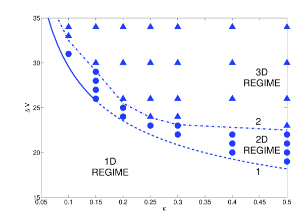
Figure 1: (Color online) Map of regimes and bifurcations, $\Delta V$ vs. $\varkappa$ for $\nu=10^{-3}$. The solid line is the neutral stability curve DemNikSh which separates the 1D and 2D regimes. Circles correspond to realizations of 2D regimes; triangles, to realization of 3D regimes, so that the 2D–3D transition happens on the dashed line.

first coordinate is the potential drop $\Delta V$ and the other is the coupling coefficient $\varkappa$. The curve 1 corresponds to the threshold of instability: for $\varkappa<0.151$, the bifurcation is supercritical and this part of 1 is pictured by the solid line; for $\varkappa>0.151$, the bifurcation is subcritical, this part of the curve is shown by the dashed line (see DemNikSh ). The 1D regimes and the limiting currents are located below 1. The circles and triangles stand for the 2D and 3D regimes, respectively. The dash-dot line 2 separates these regimes and corresponds to the 2D–3D transition.

The dependence of the average of the electric current $J$ over the membrane surface $l_{x}l_{z}=l^{2}$ and the elapsed time $t$ (see Eq.(5)) on the potential drop $\Delta V$ is a convenient integral characteristic of the regimes. Such a VC dependence is shown in Fig. 2 for a typical value of

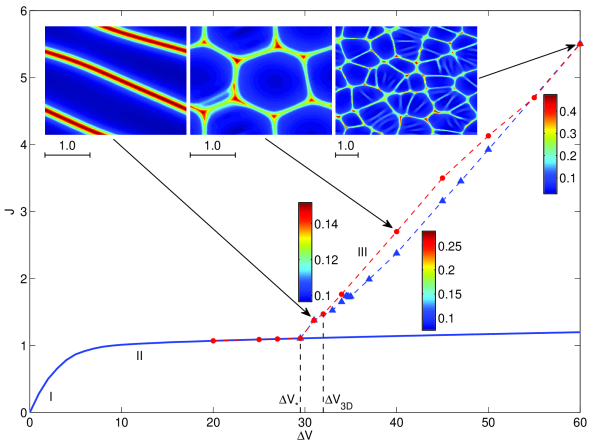
Figure 2: (Color online) VC characteristics for $\varkappa=0.1$ and $\nu=10^{-3}$: I, II and III stand for underlimiting, limiting, and overlimiting currents, respectively. The dashed line joining the circles corresponds to our 3D simulations; the dashed line joining the triangles corresponds to 2D simulations. The inset shows three typical electrokinetic patterns: 2D electroconvective rolls, regular 3D hexagonal structures, and chaotic 3D structures.

the coupling coefficient $\varkappa=0.1$, where the bifurcation is supercritical. Portions of the VC dependence, I, II and III, stand for the underlimiting, limiting, and overlimiting currents, respectively. The dashed line in Fig. 2 joining the circles corresponds to 3D simulations. We find it instructive to plot in this figure also the results of the 2D simulations; they are shown by the dashed line joining the triangles corresponding to the 2D simulations. Until the point $\Delta V=\Delta V_{\text{3D}}$, both dependences coincide. This means that for a small supercriticality, the electrokinetic instability is two-dimensional. This points to the fact that 3D effects increase the ion flux in comparison with the two-dimensional regime, but this increase is not large, about $5\%\div 10\%$. Moreover, for large enough $\Delta V$, $\Delta V>55$, this difference practically disappears.

Our simulations show that four basic coherent structures can be found during the evolution: 2D electroconvective rolls (vortices), squares, triangles, and hexagons.

1. The first coherent structure, spatially periodic stationary electroconvective rolls, can be realized as an attractor, as $t\to\infty$, only in a narrow band near the threshold of instability, between curves $1$ and $2$ of Fig. 1. This is reminiscent of the Rayleigh-Bénard convection (see CrHog ) when near the threshold hexagons and squares are unstable to rolls and there is a closed region of their stability called the “Busse balloon.” Note that the bifurcation picture is different for the Bénard–Marangoni convection, where stable hexagonal patterns can arise at the threshold (see Nep ). The two dimensional coherent structures are of particular interest because of the relative simplicity of their investigation in the 2D formulation. These solutions were analyzed in detail in DemShel ; ShelDem ; DemChang ; Han1 ; Mani ; DemNikSh .

2. For $\Delta V>\Delta V_{\text{3D}}$, above line 2 of Fig. 1, the 2D electroconvective rolls become unstable to three-dimensional perturbations. Theoretically there are three candidates to inherit stability and be a new attractor: squares, triangles, and hexagons CrHog . Our simulations show that for the electrokinetic instability, steady and regular squares and triangles do not exist: they can be seen during the evolution only as a transitional state.

3. Regular steady-state hexagonal patterns are formed just above line 2 of Fig. 1. The white noise initial perturbations eventually evolve towards steady hexagonal patterns.

4. As the driving $\Delta V-\Delta V_{*}$ is increased, the ordered hexagonal structures break down to complex and highly disordered states and the behavior becomes chaotic in time and space. The flow is a combination of unsteady hexagons, quadrangles and triangles.

To complete the VC dependence, three characteristic electrokinetic patterns are shown in the inset to Fig. 2: 2D electroconvective vortices, regular 3D hexagonal structures, and chaotic 3D structures (combinations of unsteady hexagons, quadrangles and triangles). The arrows show the place of these structures at the VC curve and a typical potential drop for their realization. A movie of the evolution of these structures can be found in Vis .

Let us consider some important details of these characteristic patterns: the electroconvective rolls, the hexagons, and the spatiotemporal chaos. In order to present a full picture of the behavior, it is instructive to analyze together the distribution of $y_{m}(x,z)$ along the membrane surface, the charge density $\rho$ inside the ESC region, and the electric current $j(x,z)$ determined by Eq. (5). Their typical snapshots are depicted in Fig. 3, Fig. 4, and Fig. 5.

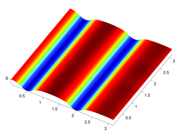
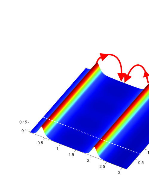
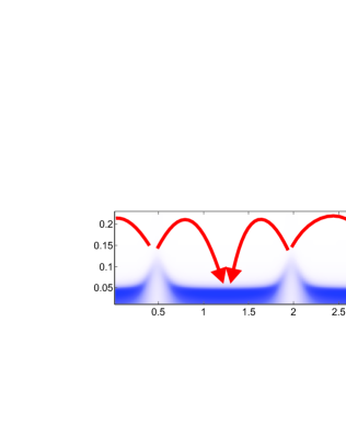
Figure 3: (Color online) Electroconvective rolls for $\Delta V=33$, $\varkappa=0.1$, and $\nu=10^{-3}$. Profile of $y_{m}(x,z)$, cross-section of charge density $\rho$ at $z=z_{*}$, and distribution of the electric current $j(x,z)$. Vortex pairs of liquid flow are shown schematically by the arrows.

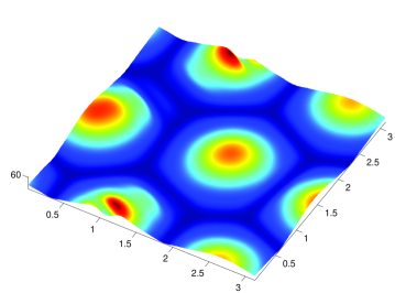
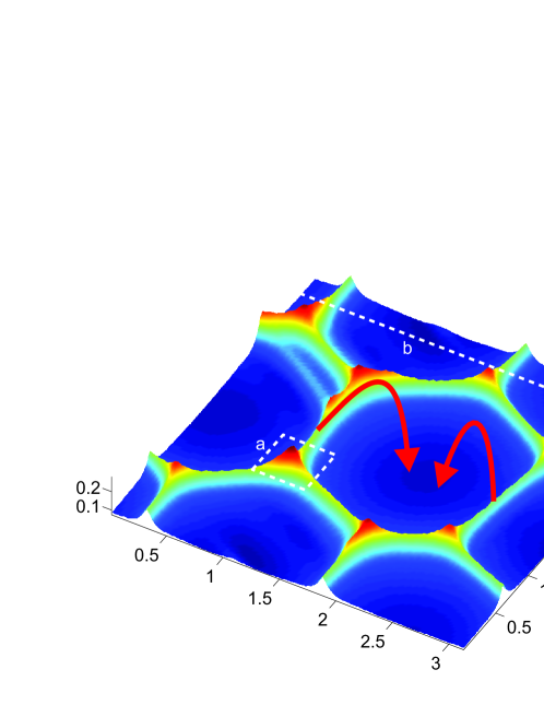
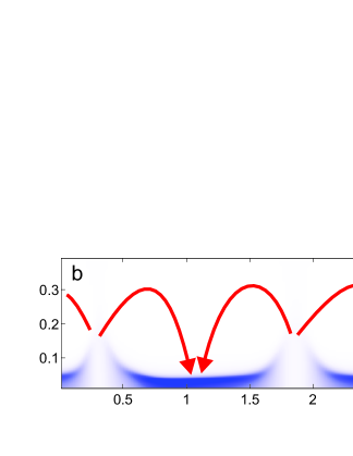
Figure 4: (Color online) Hexagonal coherent structures, $\Delta V=50$, $\varkappa=0.1$, and $\nu=10^{-3}$. Profile of ESC region, $y_{m}(x,z)$; (a) vicinity of the pyramid top; (b) cross-section $z=z_{*}$ of the charge density $\rho$. Distribution of the electric current $j(x,z)$ on the membrane surface. The arrows schematically show the direction of the liquid flow.

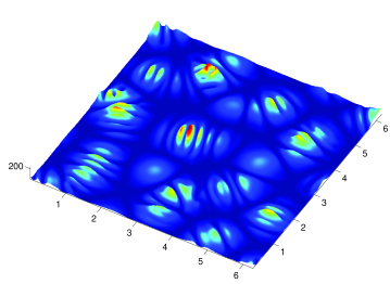
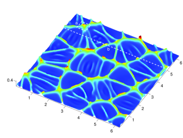
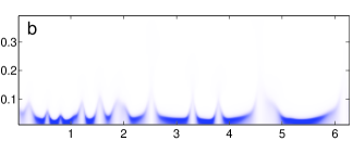
Figure 5: (Color online) Snapshot of $y_{m}$ for the spatiotemporal chaos; (a) vicinity of the pyramid top; (b) cross-section $z=z_{*}$ of the charge density $\rho$. Distribution of the electric current $j(x,z)$ on the membrane surface. $\Delta V=60$, $\varkappa=0.1$, and $\nu=10^{-3}$.

For rolls, the profile $y_{m}(x,z)$ is shown in Fig. 3; it has long flat and short wedge-like regions with a cusp at the top. The wedge angle or the angle between the wedge faces is rather conservative, it practically does not depend on the parameters and is about $105^{\circ}\div 118^{\circ}$.

After loss of stability and after the corresponding bifurcation, the rolls turn into steady three-dimensional structures, see Fig. 4; these structures are conventionally called “hexagons.” The $y_{m}(x,z)$ profile consists of six wedge-like lateral faces and six pyramids are located at their intersection. In the remaining area, $y_{m}(x,z)$ is flat and situated in the lowlands. It is interesting that the angle of wedge-like faces is close to that for the 2D rolls, and the dependence of this angle on the parameters of the problem is also weak. A rough evaluation of the pyramid angle gives its value as about $85^{\circ}\div 90^{\circ}$.

Snapshots of the spatiotemporal chaos are shown in Fig. 5. Now, the $y_{m}(x,z)$ distribution consists of a combination of triangles, quadrangles, and hexagons whose location and form change chaotically. The sides of these geometrical figures are wedges with an angle averaged over time of about $110^{\circ}$. The pyramids formed at the intersection of the sides have a time-average angle at the top of about $90^{\circ}$.

The numerical resolution of the charge density $\rho$ in the thin ESC layer is shown for our three basic patterns in the left part of Fig. 3, Fig. 4, and Fig. 5. The darker regions correspond to large charge densities $\rho$ with a rather sharp boundary between the ESC region, $0<y<y_{m}$, and the diffusion region, $y>y_{m}$. The portions with a small charge in the spikes are joined by the flat regions of large charge. For all three regimes, the minimum of $y_{m}$ corresponds to the maximum of the charge density. At the top of the pyramids, where $y_{m}(x,y)$ reaches its maximum maximorum, the $\rho$ distribution always has its minimum minimorum.

The electric current at the membrane surface, $j(x,z)$, is another important characteristic value whose description complements our understanding of the system behavior, see the top of Fig. 3, Fig. 4, and Fig. 5. For all three basic coherent structures, $j(x,z)$ qualitatively replicates the $y_{m}(x,z)$ profile and $\rho$ distribution in the ESC layer, but smooths their sharp details: for 2D rolls, the localized wedge-like profile of $y_{m}(x,z)$ turns into the nearly sinusoidal profile of $j(x,z)$; for the 3D regular patterns, the hexagon turns into a circle; the triangles, quadrangles, and hexagons of the spatiotemporal chaos transform into a system of circles and ellipses. Moreover, the electric current $j(x,z)$ has minimal values in the vicinity of the cusps and is maximal in the flat regions of the $y_{m}$ and $\rho$ distributions. We attribute this behavior to the fact that the electrical conductivity is smaller in the cusp regions and larger in the lowlands.

Our simulations show that liquid always flows upwards from the cusp points of the $y_{m}$ and $\rho$ distributions and returns to the membrane surface moving towards the flat regions of the $\rho$ distribution. An array of vortex pairs is formed; it is schematically shown in the figures by the arrows. The characteristic size of the electroconvective rolls varies within the range $1.3\div 2.0$, of the regular hexagonal structures the size is about $1.5$, and for the spatiotemporal chaos, about $1.2$.

An interesting phenomenon found is the generation of two-dimensional running solitary waves (pulses). Such waves form spontaneously either inside the hexagonal structure or at one of its lateral sides with subsequent propagation towards the opposite side of the hexagon, see Fig. 5. For relatively small drives $\Delta V-\Delta V_{*}$, the pulse generation is a rare event, moreover the pulse decays during its propagation and eventually completely disappears. As $\Delta V-\Delta V_{*}$ increases, this generation occurs more frequently, the pulse amplitude increases, and the pulse can propagate without decaying and reach the opposite side of the hexagon. If at the neighboring side or somewhere else another solitary wave forms and then departs, a complex pulse–pulse interaction occurs; depending on the spatial location of the waves, it can be a head-on or an oblique interaction. For large $\Delta V-\Delta V_{*}$, the pulse–pulse interaction becomes strong enough to destroy the hexagonal structure and a transition to spatiotemporal chaos results from the interaction. Note that similar phenomena of pulse generation and pulse–pulse interactions have been observed for other kinds of instability, Marangoni–Bénard convection Vel1 ; Vel2 and falling liquid films ChD .

Conclusions

A direct numerical simulation of the elektrokinetic instability in its three-dimensional formulation was carried out. A special numerical algorithm was developed. The calculations employed parallel computing. Three characteristic patterns, which correspond to the overlimiting currents, were observed: two-dimensional electroconvective rolls, three-dimensional regular hexagonal structures, and three-dimensional structures of spatiotemporal chaos, which are combinations of unsteady hexagons, quadrangles and triangles. The distinguishing features of the regular and chaotic three-dimensional regimes were found. The transition from the steady regular three-dimensional patterns to the spatiotemporal chaos was found to be accompanied by the generation of interacting two-dimensional solitary pulses.

References

- (1) H.-C. Chang, G. Yossifon, and E. A. Demekhin, “Nanoscale electrokinetics and microvortices: How microhydrodynamics affects nanofluidic ion flux,” Annu. Rev. Fluid Mech. 44, 401 (2012).
- (2) I. Rubinstein and B. Zaltzman, “Electro-osmotically induced convection at a permselective membrane,” Phys. Rev. E 62, 2238 (2000).
- (3) I. Rubinstein and B. Zaltzman, “Electro-osmotic slip of the second kind and instability in concentration polarization at electrodialysis membranes,” Math. Mod. Meth. Appl. Sci., 11, 263 (2001).
- (4) I. Rubinstein and B. Zaltzman, “Wave number selection in a nonequilibrium electroosmotic instability,” Phys. Rev. E 68, 032501 (2003).
- (5) I. Rubinstein, E. Staude, and O. Kedem, “Role of the membrane surface in concentration polarization at ion-exchange membrane,” Desalination 69, 101 (1988).
- (6) F. Maletzki, H. W. Rossler, and E. Staude, “Ion transfer across electrodialysis membranes in the overlimiting current range: Stationary voltage–current characteristics and current noise power spectra under different condition of free convection,” J. Membr. Sci. 71, 105 (1992).
- (7) I. Rubinshtein, B. Zaltzman, J. Pretz, and C. Linder, “Experimental verification of the electroosmotic mechanism of overlimiting conductance through a cation exchange electrodialysis membrane,” Russ. J. Electrochem. 38, 853 (2002).
- (8) S. M. Rubinstein, G. Manukyan, A. Staicu, I. Rubinstein, B. Zaltzman, R. G. H. Lammertink, F. Mugele, and M. Wessling, “Direct observation of nonequilibrium electroosmotic instability,” Phys. Rev. Lett. 101, 236101 (2008).
- (9) G. Yossifon and H.-C. Chang, “Selection of nonequilibrium overlimiting currents: Universal depletion layer formation dynamics and vortex instability,” Phys. Rev. Lett. 101, 254501 (2008).
- (10) S. J. Kim, Y.-C. Wang, J. H. Lee, H. Jang, and J. Han, “Concentration polarization and nonlinear electrokinetic flow near a nanofluidic channel,” Phys. Rev. Lett. 99, 044501.1 (2007).
- (11) B. Zaltzman and I. Rubinstein, “Electroosmotic slip and electroconvective instability,” J. Fluid Mech. 579, 173 (2007).
- (12) E. A. Demekhin, E. M. Shapar, and V. V. Lapchenko, “Initiation of electroconvection in semipermeable electric membranes,” Doklady Physics 53, 450 (2008).
- (13) E. A. Demekhin, S. V. Polyanskikh and Y. M. Shtemler, “Electroconvective instability of self-similar equilibria,” e-print arXiv: 1001.4502.
- (14) E. N. Kalaidin, S. V. Polyanskikh, and E. A. Demekhin, “Self-similar solutions in ion-exchange membranes and their stability,” Doklady Physics 55, 502 (2010).
- (15) E. A. Demekhin, V. S. Shelistov, and S. V. Polyanskikh, “Linear and nonlinear evolution and diffusion layer selection in electrokinetic instability,” Phys. Rev. E 84, 036318 (2011).
- (16) V. S. Shelistov, N. V. Nikitin, G. S. Ganchenko, and E. A. Demekhin, “Numerical modeling of electrokinetic instability in semipermeable membranes,” Dokl. Phys. 56, 538 (2011).
- (17) H.-C. Chang, E. A. Demekhin, and V. S. Shelistov “Competition between Dukhin’s and Rubinstein’s electrokinetic modes,” Phys. Rev. E 86, 046319 (2012).
- (18) V. S. Pham, Z. Li, K. M. Lim, J. K. White, and J. Han, “Direct numerical simulation of electroconvective instability and hysteretic current–voltage response of a permselective membrane,” Phys. Rev. E 86, 046310 (2012).
- (19) C. L. Druzgalski, M. B. Andersen, and A. Mani, “Direct numerical simulation of electroconvective instability and hydrodynamic chaos near an ion-selective surface,” Phys. Fluids. 25, 110804 (2013).
- (20) E. A. Demekhin, N. V. Nikitin, and V. S. Shelistov, “Direct numerical simulation of electrokinetic instability and transition to chaotic motion,” Phys. Fluids 25, 122001 (2013).
- (21) N. V. Nikitin, “Third-order-accurate semi-implicit Runge–Kutta scheme for incompressible Navier–Stokes equations,” Int. J. Num. Meth. Fluids 51(2), 221 (2006).
- (22) E. A. Demekhin N. V. Nikitin, and V. S. Shelistov, (unpublished).
- (23) I. Rubinstein and L. Shtilman, “Voltage against current curves of cation exchange membranes,” J. Chem. Soc. Faraday Trans. 2 75, 231 (1979).
- (24) M. C. Cross and P. G. Hohenberg, “Pattern formation outside of equilibrium,” Rev. Modern Physics 65, 3, 851 (1993).
- (25) A. A. Nepomnyashcy, M. G. Velarde, and P. Colinet, Interfacial Phenomena and Convection, Chapman & Hall/CRC, London, 2002.
- (26) http://demekhin.kubannet.ru/electrokinetic.php.
- (27) P. D. Wedman, H. Linde, and M. G. Velarde, “Evidence for solitary wave behavior in Marangoni–Bénard convection,” Phys. Fluids A 4, 921 (1992).
- (28) H. Linde, X. Chu, and M. G. Velarde, “Oblique and head-on collision of solitary waves in Marangoni–Bénard convection,” Phys. Fluids A 5, 1068 (1993).
- (29) H.-C. Chang, E. A. Demekhin, and E. N. Kalaidin, “Interaction dynamics of solitary waves on a falling film,” J. Fluid Mech. 294, 123 (1995).