Behaviors of Networks with Antagonistic Interactions and Switching Topologies

Abstract

In this paper, we study the discrete-time consensus problem over networks with antagonistic and cooperative interactions. A cooperative interaction between two nodes takes place when one node receives the true state of the other while an antagonistic interaction happens when the former receives the opposite of the true state of the latter. We adopt a quite general model where the node communications can be either unidirectional or bidirectional, the network topology graph may vary over time, and the cooperative or antagonistic relations can be time-varying. It is proven that, the limits of all the node states exist, and the absolute values of the node states reach consensus if the switching interaction graph is uniformly jointly strongly connected for unidirectional topologies, or infinitely jointly connected for bidirectional topologies. These results are independent of the switching of the interaction relations. We construct a counterexample to indicate a rather surprising fact that quasi-strong connectivity of the interaction graph, i.e., the graph contains a directed spanning tree, is not sufficient to guarantee the consensus in absolute values even under fixed topologies. Based on these results, we also propose sufficient conditions for bipartite consensus to be achieved over the network with joint connectivity. Finally, simulation results using a discrete-time Kuramoto model are given to illustrate the convergence results showing that the proposed framework is applicable to a class of networks with general nonlinear dynamics.

, , , ,

1 Introduction

Distributed consensus algorithms were first introduced in the study of distributed optimization methods in (Tsitsiklis et al. (1986)). Phase synchronization was observed in (Vicsek et al. (1995)) and its mathematical proof was given in (Jadbabaie et al. (2003)). The robustness of the consensus algorithm to link/node failures and time-delays was studied in (Olfati-Saber et al. (2007)). A central problem in consensus study is to investigate the influence of the interaction graph on the convergence or convergence speed of the multi-agent system dynamics. The interaction graph, which describes the information flow among the nodes, is often time-varying due to the complexity of the interaction patterns in practice. Both continuous-time and discrete-time models were studied for consensus algorithms with switching interaction graphs and joint connectivity conditions were established for linear models (Blondel et al. (2005); Ren and Beard (2005); Cao et al. (2008b); Hendrickx and Tsitsiklis (2013)). Nonlinear multi-agent dynamics have also drawn much attention (Shi and Hong (2009); Meng et al. (2013)) since in many practical problems the node dynamics are naturally nonlinear, e.g., the Kuramoto model (Strogatz (2000)).

Although great progress has been made, most of the existing results are based on the assumption that the agents in the network are cooperative. Recently, motivated by opinion dynamics over social networks (Cartwright and Harary (1956); Hegselmann and Krause (2002); Easley and Kleinberg (2010)), consensus algorithms over cooperative-antagonistic networks drew much attention (Altafini (2012, 2013); Shi et al. (2013)). Altafini (Altafini (2013)) assumed that a node receives the opposite of the true state of its neighboring node if they are antagonistic. Therefore, the modeling of such an antagonistic input for agent $i$ is of the form $-(x_{i}+x_{j})$ (in contrast to the form $-(x_{i}-x_{j})$ for cooperative input), where $j$ denotes the antagonistic neighbor of agent $i$. On the other hand, the authors of Shi et al. (2013) assumed that a node receives the opposite of the relative state from its neighboring node if they are antagonistic. Then, the antagonistic input for agent $i$ is modeled by the form $(x_{i}-x_{j})$ in this case. The extension to the case of homogenous single-input high-order dynamical systems was discussed in (Valcher and Misra (2014)). The graph was assumed to be fixed and a spectral analysis approach was used. Instead, we will focus on switching topologies with joint connectivity and take advantage of a detailed state-space analysis approach in this paper. A lifting approach was proposed in Hendrickx (2014) to study opinion dynamics with antagonisms over switching interaction graphs. Some general conditions were established by applying the rich results from the consensus literature. The dissensus problem was studied in (Bauso et al. (2012)), where the focus was to understand when consensus is or is not achieved if death and duplication phenomena occur. Note that in dissensus the control terms for death and duplication phenomena are added to the classical consensus algorithm. However, consensus or bipartite consensus in our study does not denote a control goal, but a final behavior of multi-agent systems. In particular, consensus denotes the final states of all the agents converging to the same value while bipartite consensus denotes the final states of all the agents converging to two opposite values.

Note that most of the existing works on antagonistic interactions are based on the assumption that the interaction graph is fixed. In many practical cases, however, the interactions between agents may vary over time or be dependent on the states. In this paper, we focus on the behavior of multiple agents with antagonistic interactions, discrete-time dynamics, and switching interaction graphs. Both unidirectional and bidirectional topologies are considered. We show that the limits of all node states exist and reach a consensus in absolute values if the switching interaction graph is uniformly jointly strongly connected for unidirectional topologies, or infinitely jointly connected for bidirectional topologies. Here, reaching consensus in absolute values is not a design objective, but rather an emergent behavior that we can observe for cooperative-antagonistic networks. By noting that an antagonistic interaction also represents an arc in the graph, we know that the connectivity of the network may not be guaranteed without antagonistic interactions. Therefore, we actually show that the antagonistic interaction has a similar role as the cooperative interaction in contributing to the consensus of the absolute values of the node states. In addition, a counterexample is constructed that indicates that quasi-strong connectivity of the interaction graph, i.e., the graph has a directed spanning tree, is not sufficient to guarantee consensus of the node states in absolute values even under a fixed topology. Based on these results, we propose sufficient conditions for bipartite consensus to be achieved over a network with joint connectivity. It turns out that the structural balance condition is essentially important and this part of the result can be viewed as an extension of the work Altafini (2013) to the case of general time-varying graphs with joint connectivity. A detailed asymptotic analysis is performed with a contradiction argument to show the main results.

2 Problem Formulation and Main Results

Consider a multi-agent network with agent set $\mathcal{V}=\{1,\dots,n\}$. In the rest of the paper we use agent and node interchangeably. The state-space for the agents is $\mathbb{R}$, and we let $x_{i}\in\mathbb{R}$ denote the state of node $i$. Set $x=(x_{1},x_{2},\dots,x_{n})^{\rm\tiny T}$.

2.1 Interaction Graph

The interaction graph of the network is defined as a sequence of unidirectional graphs, $\mathcal{G}_{k}=(\mathcal{V},\mathcal{E}_{k})$, $k=0,1,\dots$, with node set $\mathcal{V}$ and $\mathcal{E}_{k}\subseteq\mathcal{V}\times\mathcal{V}$ is the set of arcs at time $k$. An arc from node $i$ to $j$ is denoted by $(i,j)$. A path from node $i$ to $j$ is a sequence of consecutive arcs $\{(i,k_{1}),\dots,(k_{l},j)\}$. We assume that $\mathcal{G}_{k}$ is a signed graph, where “+” or “$-$” is associated with each arc $(i,j)\in\mathcal{E}_{k}$. Here, “+” represents cooperative relation and “$-$” represents antagonistic relation. The set of neighbors of node $i$ in $\mathcal{G}_{k}$ is denoted by $\mathcal{N}_{i}(k):=\{j:(j,i)\in\mathcal{E}_{k}\}\cup\{i\}$, and $\mathcal{N}_{i}^{+}(k)$ and $\mathcal{N}^{-}_{i}(k)$ are used to denote the cooperative neighbor sets and antagonistic neighbor sets, respectively. Clearly, $\mathcal{N}_{i}(k)=\mathcal{N}_{i}^{-}(k)\cup\mathcal{N}_{i}^{+}(k)\cup\{i\}$. The joint graph of $\mathcal{G}$ during time interval $[k_{1},k_{2})$ is defined by $\mathcal{G}([k_{1},k_{2}))=\bigcup_{k\in[k_{1},k_{2})}\mathcal{G}_{k}=(\mathcal{V},\bigcup_{k\in[k_{1},k_{2})}\mathcal{E}_{k})$. The sequence of graphs $\{\mathcal{G}_{k}\}_{0}^{\infty}$ is said to be sign consistent if the sign of any arc $(i,j)$ does not change over time. Under the assumption that $\{\mathcal{G}_{k}\}_{0}^{\infty}$ is sign consistent, we can define a signed total graph $\mathcal{G}^{*}:=(\mathcal{V},\mathcal{E}^{*})$, where $\mathcal{E}^{*}=\cup_{k=0}^{\infty}\mathcal{E}_{k}$.

We write $i\rightarrow j$ if there is a path from $i$ to $j$. A root is a node $i$ such that $i\rightarrow j$ for every other node $j\in\mathcal{V}\backslash\{i\}$. A unidirectional graph is quasi-strongly connected if it has a directed spanning tree, i.e., there exists at least one root. A unidirectional graph is called strongly connected if there is a path connecting any two distinct nodes. A unidirectional graph $\mathcal{G}$ is called bidirectional if for any two nodes $i$ and $j$, $(j,i)\in\mathcal{E}$ if and only if $(i,j)\in\mathcal{E}$. A bidirectional graph is connected if it is connected as a bidirectional graph ignoring the arc directions. We introduce the following definition of the joint connectivity of a sequence of graphs.

Definition 2.1.

(i). $\{\mathcal{G}_{k}\}_{0}^{\infty}$ is uniformly jointly strongly connected if there exists a constant $T\geq 1$ such that $\mathcal{G}([k,k+T))$ is strongly connected for any $k\geq 0$.

(ii). $\{\mathcal{G}_{k}\}_{0}^{\infty}$ is uniformly jointly quasi-strongly connected if there exists a constant $T\geq 1$ such that $\mathcal{G}([k,k+T))$ has a directed spanning tree for any $k\geq 0$.

(iii). Suppose $\mathcal{G}_{k}$ is bidirectional for all $k\geq 0$. Then $\{\mathcal{G}_{k}\}_{0}^{\infty}$ is infinitely jointly connected if $\mathcal{G}([k,+\infty))$ is connected for any $k\geq 0$.

2.2 Node Dynamics

The update rule for each node is described by:

$$x_{i}(k+1)= \sum_{j\in\mathcal{N}_{i}(k)}a_{ij}(x,k)x_{j}(k),$$

$$k=0,1,\dots,\quad i=1,2,\dots,n,$$ (1)

where $x_{i}(k)\in\mathbb{R}$ represents the state of agent $i$ at time $k$, $x=(x_{1},x_{2},\dots,x_{n})^{\rm\tiny T}$, and $a_{ij}(x,k)$ represents a nonlinear time-varying function. Equation (1) can be written in the compact form:

$$x(k+1)=A(x,k)x(k),\quad k=0,1,\dots,$$ (2)

where $A(x,k)=[a_{ij}(x,k)]\in\mathbb{R}^{n\times n}$. For $a_{ij}(x,k)$, we impose the following assumption.

Assumption 2.1.

There exists a positive constant $0<\lambda<1$ such that:

(i) $a_{ii}(x,k)\geq\lambda$, for all $i,x,k$, and $\sum_{j\in\mathcal{N}_{i}(k)}|a_{ij}(x,k)|=1$ for all $i,x,k$;

(ii) $a_{ij}(x,k)\geq\lambda$ for all $i,j,x,k$, if $j\in\mathcal{N}_{i}^{+}(k)$; and $a_{ij}(x,k)\leq-\lambda$ for all $i,j,x,k$, if $j\in\mathcal{N}_{i}^{-}(k)$.

Remark 2.1.

The antagonistic interactions commonly exist in social networks and signed graphs are used to describe these interactions. In signed graphs, a positive/negative weight is associated with a cooperative/antagonistic relationship between the two agents. Assumption 2.1 models such a signed graph in a discrete-time dynamics and switching topology setting. Similar modeling can be found in Altafini (2013) with continuous-time dynamics and fixed topology. Clearly, the second part of Assumption 2.1 describes cooperative-antagonistic interactions in the sense that $a_{ij}(x,k)>0$ represents that $i$ is cooperative to $j$, and $a_{ij}(x,k)<0$ represents that $i$ is antagonistic to $j$. In addition, because of complexity of the interaction patterns, $a_{ij}$ may depend on time or relative measurements for agent dynamics (2), instead of being constant. Lots of practical multi-agent system models can be written in this form (e.g., Kuramoto equation, consensus algorithm, and swarming model given in Moreau (2005)). Last but not the least, we want to emphasize that the existence of a positive constant $\lambda$ in Assumption 2.1 is a technical assumption and plays an indispensable role in driving the states of the system asymptotically to converge (see the proofs of the main theorems). This is in fact a very general assumption and has been used extensively in the existing literature (see e.g., Blondel et al. (2005); Shi et al. (2013)). Here, $\lambda$ can be an arbitrarily small constant and thus the assumption on the existence of $\lambda$ will not restrict the usefulness of Assumption 2.1 on practical applications.

2.3 Main Results

Uniform joint strong connectivity is sufficient for convergence of agent states for unidirectional graphs, as stated in the following theorem.

Theorem 2.1.

Suppose that Assumption 2.1 holds and that $\mathcal{G}_{k}$ is unidirectional for all $k\geq 0$. For system (1), $\lim_{k\rightarrow\infty}x_{i}(k)$ exists and $\lim_{k\rightarrow\infty}|x_{i}(k)|=M^{*}$, for all $i\in\mathcal{V}$ and every initial state $x(0)\in\mathbb{R}^{n}$, if $\{\mathcal{G}_{k}\}_{0}^{\infty}$ is uniformly jointly strongly connected, where $M^{*}$ is a nonnegative constant.

For cooperative networks, it is well-known that asymptotic consensus can be achieved if the interaction graph is uniformly quasi-strongly connected, e.g., (Ren and Beard (2005); Cao et al. (2008a)). Note that quasi-strong connectedness is weaker than strong connectedness. Then, a natural question is whether asymptotic consensus in absolute values can be achieved when the interaction graph is uniformly quasi-strongly connected. We construct the following counterexample showing that quasi-strong connectivity is not sufficient for the consensus in absolute values even in case of a fixed graph.

Counterexample. Let $\mathcal{V}=\{1,2,3\}$ and initial state is $x(0)=(1,0,-1)^{\rm\tiny T}$. The interaction graph $\mathcal{G}_{k}=\mathcal{G}$ is fixed and shown in Fig. 1 and

$$A=[a_{ij}]=\left[\begin{matrix}1&0&0\\ 1/3&1/3&1/3\\ -1/2&0&1/2\end{matrix}\right].$$

It is straightforward to check that $\mathcal{G}$ is quasi-strongly connected. However, the states of the agents remain $x_{1}(k)=1$, $x_{2}(k)=0$, and $x_{3}(k)=-1$, for all $k=1,2,\dots$ under system dynamics (1). Thus, the absolute values of the agent states do not reach a consensus.

Figure 1: Signed graph $\mathcal{G}$ used in the counterexample

For bidirectional graphs, we present the following result indicating that the consensus in absolute values can be achieved under weaker connectivity conditions than those in Theorem 2.1 for unidirectional graphs.

Theorem 2.2.

Suppose that Assumption 2.1 holds and $\mathcal{G}_{k}$ is bidirectional for all $k\geq 0$. For system (1), $\lim_{k\rightarrow\infty}x_{i}(k)$ exists and $\lim_{k\rightarrow\infty}|x_{i}(k)|=M^{*}$, for all $i\in\mathcal{V}$ and every initial state $x(0)\in\mathbb{R}^{n}$ if $\{\mathcal{G}_{k}\}_{0}^{\infty}$ is infinitely jointly connected, where $M^{*}$ is a nonnegative constant.

We note that Theorems 2.1 and 2.2 are concerned with consensus of the absolute values of agent states. It is not clear what is the final sign of the states, i.e., the sign of $\lim_{k\rightarrow\infty}x_{i}(k)$ for different $i\in\mathcal{V}$. We next characterize how bipartite consensus, i.e., splitting into two opposite states, can emerge. We first introduce the notion of structural balance, cf., Definition 2 of Altafini (2013).

Definition 2.2.

Suppose that the sequence of graphs $\{\mathcal{G}_{k}\}_{0}^{\infty}$ is sign consistent and $\mathcal{G}^{*}=(\mathcal{V},\mathcal{E}^{*})$ is a signed total graph defined in Section 2.1. $\mathcal{G}^{*}$ is structurally balanced if we can divide $\mathcal{V}$ into two disjoint nonempty subsets $\mathcal{V}_{1}$ and $\mathcal{V}_{2}$ (i.e., $\mathcal{V}_{1}\bigcup\mathcal{V}_{2}=\mathcal{V}$ and $\mathcal{V}_{1}\bigcap\mathcal{V}_{2}=\emptyset$), where negative arcs only exist between these two subsets, i.e., the arc $(i,j)$ is associated with sign “+”, $\forall i,j\in\mathcal{V}_{q}$ ($q\in\{1,2\}$) and the arc $(i,j)$ is associated with sign “$-$”, $\forall i\in\mathcal{V}_{q},j\in\mathcal{V}_{r},q\neq r$ ($q,r\in\{1,2\}$).

Remark 2.2.

Since we assume that the sequence of graphs $\{\mathcal{G}_{k}\}_{0}^{\infty}$ is sign consistent, even if the interconnection graph may be changing with time, the sets ${\mathcal{V}}_{1}$ and ${\mathcal{V}}_{2}$ do not, and hence the two “antagonistic groups” are always the same given that the signed total graph $\mathcal{G}^{*}$ is structurally balanced.

We next establish our result for bipartite consensus.

Theorem 2.3.

Suppose that $\mathcal{G}_{k}$ is unidirectional for all $k\geq 0$ and $\{\mathcal{G}_{k}\}_{0}^{\infty}$ is uniformly jointly strongly connected, or $\mathcal{G}_{k}$ is bidirectional for all $k\geq 0$ and $\{\mathcal{G}_{k}\}_{0}^{\infty}$ is infinitely jointly connected. Also suppose that Assumption 2.1 holds, $\mathcal{G}^{*}$ is structurally balanced, and every negative arc in $\mathcal{G}^{*}$ appears infinitely often in $\{\mathcal{G}_{k}\}_{0}^{\infty}$. For system (1), $\lim_{k\rightarrow\infty}x_{i}(k)=M^{*}$, $i\in\mathcal{V}_{1}$, and $\lim_{k\rightarrow\infty}x_{i}(k)=-M^{*}$, $i\in\mathcal{V}_{2}$, for every initial state $x(0)\in\mathbb{R}^{n}$ , where $M^{*}$ is a constant.

Remark 2.3.

The interpretation of Theorem 2.3 is that under proper graph structure, the agent states in the same cooperative subgroup converge to the same limit and the limits of agents in different cooperative subgroups are exactly opposite. It is not hard to see from Theorem 2.3 that the structural balance condition plays a key role in obtaining such a bipartite consensus behavior. Theorem 2.3 can be viewed as an extension of the result of Altafini (2013) from fixed to switching graphs. We establish conditions for both unidirectional and bidirectional graphs with joint connectivity. A detailed analysis of the asymptotic behavior will be done and a contradiction argument applied to show the main results, in contrast to the spectral analysis approach given in Altafini (2013).

3 Proofs

In this section, we present the proofs of the statements. First a key technical lemma is established, and then the proofs of Theorems 2.1, 2.2, and 2.3 are presented. Since the proofs do not rely on whether or not $a_{ij}$ depends on $x$, without loss of generality, we use $a_{ij}(k)$ to denote $a_{ij}(x,k)$.

Lemma 1.

Suppose that Assumption 2.1 holds. For system (1), it holds that $\|x(k+1)\|_{\infty}\leq\|x(k)\|_{\infty}$, for all $k=0,1,\dots$.

Proof 3.1.

It follows from Assumption 2.1 that $|x_{i}(k+1)|\leq~{}\sum_{j\in\mathcal{N}_{i}(k)}|a_{ij}(k)||x_{j}(k)|\leq~{}\left(\sum_{j\in\mathcal{N}_{i}(k)}|a_{ij}(k)|\right)\\ \times\max_{i\in\mathcal{V}}|x_{i}(k)|=~{}\|x(k)\|_{\infty},$ for all $i$, which leads to the conclusion directly.

3.1 Proof of Theorem 2.1: Consensus in Absolute Values

Since a bounded monotone sequence always admits a limit, Lemma 1 implies that for any initial value $x(0)$, there exists a constant $M^{*}$, such that $\lim_{k\rightarrow\infty}\|x(k)\|_{\infty}=M^{*}$. We further define $\Phi_{i}=\limsup_{k\rightarrow\infty}|x_{i}(k)|,~{}\Psi_{i}=\liminf_{k\rightarrow\infty}|x_{i}(k)|,$ for all $i\in\mathcal{V}$. Clearly, it must hold that $0\leq\Psi_{i}\leq\Phi_{i}\leq M^{*}$. Therefore, $\lim_{k\rightarrow\infty}|x_{i}(k)|=M^{*}$, for all $i\in\mathcal{V}$ if and only if $\Phi_{i}=\Psi_{i}=M^{*}$, $i\in\mathcal{V}$.

In addition, based on the fact that $\lim_{k\rightarrow\infty}\|x(k)\|_{\infty}=M^{*}$, it follows that for any $\varepsilon>0$, there exists a $\widehat{k}(\varepsilon)>0$ such that $M^{*}-\varepsilon\leq\|x(k)\|_{\infty}\leq M^{*}+\varepsilon$, $\forall k\geq\widehat{k}(\varepsilon)$ and $|x_{i}(k)|\leq M^{*}+\varepsilon,~{}~{}\forall i\in\mathcal{V},~{}~{}\forall k\geq\widehat{k}(\varepsilon).$

We next use a contradiction argument. Now suppose that there exists a node ${i_{1}}\in\mathcal{V}$ such that $0\leq\Psi_{i_{1}}<M^{*}$. With the definitions of $\Psi_{i_{1}}$, for any $\varepsilon>0$, there exists a constant $\Psi_{i_{1}}<\alpha_{1}<M^{*}$ and a time instance $k_{1}\geq\widehat{k}(\varepsilon)$ such that $|x_{i_{1}}(k_{1})|\leq\alpha_{1}$. This shows that

$$|x_{i_{1}}(k_{1})|\leq M^{*}-(M^{*}-\alpha_{1})=M^{*}-\xi_{1},$$ (3)

where $\xi_{1}=M^{*}-\alpha_{1}>0$.

First of all, it follows from Lemma 1 that $|x_{j}(k_{1}+s)|\leq\|x(k_{1})\|_{\infty}$, for all $s=1,2,\dots$ and all $j\in\mathcal{V}$. We next fix $i_{1}$ and analyze the trajectory of $x_{i_{1}}$ after $k_{1}$. Then it must be true that for all $s=1,2,\dots$, $|x_{i_{1}}(k_{1}+s)|\leq~{}\sum_{j\in\mathcal{N}_{i_{1}}(k_{1}+s-1)}\left|a_{i_{1}j}(k_{1}+s-1)\right|\left|x_{j}(k_{1}+s-1)\right|\\ =~{}\left|a_{i_{1}i_{1}}(k_{1}+s-1)\right|\left|x_{i_{1}}(k_{1}+s-1)\right|\\ +\sum_{j\in\mathcal{N}_{i_{1}}(k_{1}+s-1)\setminus\{i_{1}\}}|a_{i_{1}j}(k_{1}+s-1)||x_{j}(k_{1}+s-1)|\leq~{}|a_{i_{1}i_{1}}(k_{1}+s-1)||x_{i_{1}}(k_{1}+s-1)|+(1-|a_{i_{1}i_{1}}(k_{1}+s-1)|)\|x(k_{1})\|_{\infty}.$ Also note that $\|x(k_{1})\|_{\infty}\leq M^{*}+\varepsilon$. It thus follows from (3) that

$$|x_{i_{1}}(k_{1}+1)|$$

$$\leq~{}|a_{i_{1}i_{1}}(k_{1})||x_{i_{1}}(k_{1})|+(1-|a_{i_{1}i_{1}}(k_{1})|)\|x(k_{1})\|_{\infty}$$

$$\leq~{}a_{i_{1}i_{1}}(k_{1})(M^{*}-\xi_{1})+(1-a_{i_{1}i_{1}}(k_{1}))(M^{*}+\varepsilon)$$

$$\leq~{}M^{*}+\varepsilon-\lambda\xi_{1},$$ (4)

where we have used the fact that $a_{i_{1}i_{1}}\geq\lambda$ from Assumption 2.1.

By a recursive analysis we can further deduce that

$$|x_{i_{1}}(k_{1}+s)|\leq M^{*}+\varepsilon-\lambda^{s}\xi_{1},\quad s=1,2,\dots.$$ (5)

Next, we consider the time interval $[k_{1},k_{1}+T)$. Since $\mathcal{G}([k_{1},k_{1}+T))$ is strongly connected, there is a path from $i_{1}$ to any other node during the time interval $[k_{1},k_{1}+T)$. This implies that there exists a time instant $k_{2}\in[k_{1},k_{1}+T)$ such that $i_{1}$ is a neighbor of another node $i_{2}$ at $k_{2}$. We next analyze the trajectory of $x_{i_{2}}$ after $k_{2}$. It follows that $|x_{i_{2}}(k_{2}+s)|\leq~{}\sum_{j\in\mathcal{N}_{i_{2}}(k_{2}+s-1)}|a_{i_{2}j}(k_{2}+s-1)||x_{j}(k_{2}+s-1)|=~{}|a_{i_{2}i_{1}}(k_{2}+s-1)||x_{i_{1}}(k_{2}+s-1)|+\sum_{j\in\mathcal{N}_{i_{2}}(k_{2}+s-1)\setminus\{i_{1}\}}\!\!|a_{i_{2}j}(k_{2}+s-1)||x_{j}(k_{2}+s-1)|\leq~{}|a_{i_{2}i_{1}}(k_{2}+s-1)||x_{i_{1}}(k_{2}+s-1)|+(1-|a_{i_{2}i_{1}}(k_{2}+s-1)|)\|x(k_{2})\|_{\infty},$ where we have used the fact that $|x_{i}(k_{2}+s)|\leq\|x(k_{2})\|_{\infty}$, for all $s=1,2,\dots$, and for all $i\in\mathcal{V}$. Noting that $\|x(k_{2})\|_{\infty}\leq M^{*}+\varepsilon$, it thus follows that $|x_{i_{2}}(k_{2}+s)|\leq~{}|a_{i_{2}i_{1}}(k_{2}+s-1)|(M^{*}+\varepsilon-\lambda^{s-1+k_{2}-k_{1}}\xi_{1})+(1-|a_{i_{2}i_{1}}(k_{2}+s-1)|)(M^{*}+\varepsilon)\leq~{}M^{*}+\varepsilon-\lambda^{s+k_{2}-k_{1}}\xi_{1},~{}s=1,2,\dots.$ We can further use the fact $k_{2}-k_{1}<T$ to obtain

$$|x_{i_{2}}(k_{1}+s)|\leq M^{*}+\varepsilon-\lambda^{s}\xi_{1},\ \ s=T,T+1,\dots.$$ (6)

We now reiterate the previous argument for the time interval $[k_{1}+T,k_{1}+2T)$. Again, there is a path from $i_{1}$ to any other node during the time interval $[k_{1}+T,k_{1}+2T)$. There exists a time instant $k_{3}\in[k_{1}+T+1,k_{1}+2T)$ such that either $i_{1}$ or $i_{2}$ is a neighbor of $i_{3}$ ($i_{3}$ is another node different from $i_{1}$ and $i_{2}$) at $k_{3}$. For any of the two cases we can deduce from (5) and (6) that for agent $i_{3}$, it must hold $|x_{i_{3}}(k_{1}+s)|\leq~{}M^{*}+\varepsilon-\lambda^{s}\xi_{1},\ \ s=2T,2T+1,\dots.$

The above analysis can be carried out to intervals $[k_{1}+2T,k_{1}+3T),\dots,[k_{1}+(n-2)T,k_{1}+(n-1)T)$, where $i_{4},\dots,i_{n}$ can be found recursively until they include the whole network. We can therefore finally arrive at $\|x(k_{1}+(n-1)T)\|_{\infty}\leq~{}M^{*}+\varepsilon-\lambda^{(n-1)T}\xi_{1}<~{}M^{*}-{\lambda^{(n-1)T}\xi_{1}}/{2},$ for sufficient small $\varepsilon$ satifying $\varepsilon<{\lambda^{(n-1)T}\xi_{1}}/{2}$. Then, it follows from Lemma 1 that

$$\|x(k)\|_{\infty}<M^{*}-{\lambda^{(n-1)T}\xi_{1}}/{2},$$

for all $k\geq k_{1}+(n-1)T$, which contradicts the fact that $\lim_{k\rightarrow\infty}\|x(k)\|_{\infty}=M^{*}$. Therefore, $\lim_{k\rightarrow\infty}|x_{i}(k)|=M^{*}$, for all $i\in\mathcal{V}$.

3.2 Proof of Theorem 2.1: Existence of State Limits

In this section, we show that $\lim_{k\rightarrow\infty}x_{i}(k)$ exists, for all $i\in\mathcal{V}$. Without loss of generality, $M^{*}$ is assumed to be nonzero and we fix any $i\in\mathcal{V}$. Note that the fact that $\lim_{k\rightarrow\infty}|x_{i}(k)|=M^{*}$ include three possibilities: $\lim_{k\rightarrow\infty}x_{i}(k)=M^{*}$, $\lim_{k\rightarrow\infty}x_{i}(k)=-M^{*}$, or $x_{i}(k)$ switches between $-M^{*}$ and $M^{*}$ infinitely as $k\rightarrow\infty$. The last possibility actually means $\liminf_{k\rightarrow\infty}x_{i}(k)=-M^{*}$ and $\limsup_{k\rightarrow\infty}x_{i}(k)=M^{*}$. We next prove the existence of the limit of $x_{i}(k)$ by showing that this last possibility cannot happen.

Suppose that we do have $\liminf_{k\rightarrow\infty}x_{i}(k)=-M^{*}$, and $\limsup_{k\rightarrow\infty}x_{i}(k)=M^{*}$. The following proof is based on a contradiction argument. We first use $M^{*}$ and $x_{i}(k)$ to bound the trajectory of $x_{i}$ after time instant $k$. Note that for all $s=1,2,\dots,$

$$x_{i}(k+s)= ~{}\sum_{j\in\mathcal{N}_{i}(k+s-1)}a_{ij}(k+s-1)x_{j}(k+s-1)$$

$$\leq ~{}a_{ii}(k+s-1)x_{i}(k+s-1)$$

$$+\!\!\!\!\!\!\!\!\sum_{j\in\mathcal{N}_{i}(k+s-1)\setminus\{i\}}\!\!\!\!\!\!|a_{ij}(k+s-1)||x_{j}(k+s-1)|$$

$$\leq ~{}a_{ii}(k+s-1)x_{i}(k+s-1)$$

$$+(1-a_{ii}(k+s-1))\|x(k)\|_{\infty}.$$

It thus follows that $x_{i}(k+1)\leq\lambda x_{i}(k)+(1-\lambda)\|x(k)\|_{\infty}.$ Therefore, for all $k\geq\widehat{k}(\varepsilon)$, it follows that $x_{i}(k+1)\leq\lambda x_{i}(k)+(1-\lambda)(M^{*}+\varepsilon).$ By a recursive analysis, we know that for all $k\geq\widehat{k}(\varepsilon)$ and all $s=1,2,\dots$,

$$x_{i}(k+s)\leq ~{}\lambda^{s}x_{i}(k)+(1-\lambda^{s})(M^{*}+\varepsilon).$$ (7)

Since $\liminf_{k\rightarrow\infty}x_{i}(k)=-M^{*}$, for any given $\varepsilon$, there exists an infinite sequence $\{\bar{k}_{\chi}\}_{\chi=0}^{\infty}$ such that $\bar{k}_{\chi}>\widehat{k}(\varepsilon)$ and $x_{i}(\bar{k}_{\chi})\leq-(M^{*}-\varepsilon)$, $\chi=0,1,\dots$. In addition, since $\limsup_{k\rightarrow\infty}x_{i}(k)=M^{*}$, for any $\bar{k}_{\chi}\in\{\bar{k}_{\chi}\}_{\chi=0}^{\infty}$, there exists a time instant $\bar{k}_{\overline{\chi}}>\bar{k}_{\chi}$ such that $x_{i}({\bar{k}}_{\overline{\chi}})\geq(M^{*}-\varepsilon)$. By also noting that the state at each step is bounded by the previous step from (7), there must exist a time instant $\bar{k}^{*}_{\chi}\in[\bar{k}_{\chi},\bar{k}_{\overline{\chi}}]$ such that $-\lambda(M^{*}-\varepsilon)+(1-\lambda)(M^{*}+\varepsilon)\leq x_{i}(\bar{k}^{*}_{\chi})\leq~{}-\lambda^{2}(M^{*}-\varepsilon)+(1-\lambda^{2})(M^{*}+\varepsilon)$.

Therefore, for all $\bar{k}_{\chi}$, it follows that

$$|x_{i}(\bar{k}^{*}_{\chi})|\leq ~{}\max\{|(1-2\lambda)M^{*}+\varepsilon|,|(1-2\lambda^{2})M^{*}+\varepsilon|\}$$

$$\leq ~{}M^{*}-(1-\max\{|1-2\lambda|,|1-2\lambda^{2}|\})M^{*}+\varepsilon$$

$$< ~{}M^{*}-\frac{(1-\max\{|1-2\lambda|,|1-2\lambda^{2}|\})M^{*}}{2}$$

if $\varepsilon$ is chosen sufficiently small as

$$\varepsilon<\frac{(1-\max\{|1-2\lambda|,|1-2\lambda^{2}|\})M^{*}}{2}.$$

This contradicts the fact that $\lim_{k\rightarrow\infty}|x_{i}(k)|=M^{*}$ (which was shown in the beginning of Section 3.1) and verifies that $\lim_{k\rightarrow\infty}x_{i}(k)$ exists. Therefore, we have proven Theorem 2.1.

3.3 Proof of Theorem 2.2

In this case, since $\mathcal{G}$ is infinitely jointly connected, the union graph $\mathcal{G}([k_{1},\infty])$ is connected. We can therefore define $k_{2}:=\inf_{k}\big{\{}k\geq k_{1},\mathcal{N}_{i_{1}}(k)\setminus\{i_{1}\}\neq\emptyset\big{\}}.$ We denote $\mathcal{V}_{1}=\mathcal{N}_{i_{1}}(k_{2})$. Obviously, we have that $|x_{i_{1}}(k_{2})|=|x_{i_{1}}(k_{1})|\leq M^{*}-\xi_{1}$, where $\xi_{1}=M^{*}-\alpha_{1}>0$ is defined as in (3). Therefore, following the similar analysis by which we obtained (5) and (6), we know that $|x_{i}(k_{2}+1)|\leq M^{*}+\varepsilon-\lambda\xi_{1},\ i\in\mathcal{V}_{1}.$

Similarly, since the union graph $\mathcal{G}([k_{2}+1,\infty])$ is connected, we can continue to define $k_{3}:=\inf_{k}\Big{\{}k\geq k_{2}+1:\bigcup_{i\in\mathcal{V}_{1}}\left(\mathcal{N}_{i}(k)\setminus\{i\}\right)\neq\emptyset\Big{\}}.$ We also denote $\mathcal{V}_{2}=\bigcup_{i\in\mathcal{V}_{1}}\mathcal{N}_{i}(k_{3})$. Note that $\{i_{1}\}\subseteq\mathcal{V}_{1}\subseteq\mathcal{V}_{2}$ with the definition of neighbor sets. The fact that the graph is bidirectional guarantees that $k_{3}$ is not only the first time instant that there is an arc from ${\mathcal{V}_{1}}$ to another node, but also the first time instant that there is an arc from another node to ${\mathcal{V}_{1}}$ during the time interval $[k_{2}+1,k_{3}]$. Therefore, we can apply Lemma 1 to the subset $\mathcal{V}_{1}$ for time interval $[k_{2}+1,k_{3}]$, and deduce that $|x_{i}(k_{3})|\leq M^{*}+\varepsilon-\lambda\xi_{1},\ i\in{\mathcal{V}_{1}}.$ It then follows from the same analysis that $|x_{i}(k_{3}+1)|\leq M^{*}+\varepsilon-\lambda^{2}\xi_{1},\ i\in\mathcal{V}_{2}.$

The above argument can be carried out recursively for $\mathcal{V}_{3}$, $\mathcal{V}_{4}$, $\dots$ until $\mathcal{V}_{m}=\mathcal{V}$ for some constant $m\leq n-1$. The corresponding $k_{m}$ can be found based on infinite joint connectedness condition, where $|x_{i}(k_{m}+1)|\leq M^{*}+\varepsilon-\lambda^{m}\xi_{1}$, for all $i\in\mathcal{V}$. This indicates that

$$\|x(k_{m}+1)\|_{\infty}\leq~{}M^{*}+\varepsilon-\lambda^{m}\xi_{1}<M^{*}-\lambda^{m}\xi_{1}/2,$$

for sufficient small $\varepsilon$ satisfying $\varepsilon<\lambda^{n-1}\xi_{1}/2$. This contradicts the fact that $\|x(k)\|_{\infty}\geq M^{*}-\varepsilon>M^{*}-\lambda^{m}\xi_{1}/2$, $\forall k\geq\widehat{k}(\varepsilon)$ (which was shown in the beginning of Section 3.1). Therefore, it follows that $\lim_{k\rightarrow\infty}|x_{i}(k)|=M^{*}$, for all $i\in\mathcal{V}$.

Note that the proof given in Section 3.2 does not require connectivity. Therefore, using the same analysis as Section 3.2, we can show that $\lim_{k\rightarrow\infty}x_{i}(k)$ exists, for all $i\in\mathcal{V}$. Therefore, we have proven Theorem 2.2.

3.4 Proof of Theorem 2.3

It follows from Theorem 2.1 that there exists a positive constant $M^{*}$ such that for all $i\in\mathcal{V}$, either $\lim_{k\rightarrow\infty}x_{i}(k)=M^{*}$ or $\lim_{k\rightarrow\infty}x_{i}(k)=-M^{*}$. We can therefore define two subsets of $\mathcal{V}$ as $\overline{\mathcal{V}}_{1}=\{i\in\mathcal{V}:\lim_{k\rightarrow\infty}x_{i}(k)=-M^{*}\},$ and $\overline{\mathcal{V}}_{2}=\{i\in\mathcal{V}:\lim_{k\rightarrow\infty}x_{i}(k)=M^{*}\}.$ Without loss of generality, we assume that $\overline{\mathcal{V}}_{1}$ is nonempty. Since the signed graph $\mathcal{G}^{*}=(V,\mathcal{E}^{*})$ is sign consistent, the sign of each arc $(i,j)\in\mathcal{E}^{*}$ is denoted by $\varrho_{ij}$, where $\varrho_{ij}=+$ or $\varrho_{ij}=-$. We next show that if $(i,j)\in\mathcal{E}^{*}$ and $i,j\in\overline{\mathcal{V}}_{1}$, it is necessary that $\varrho_{ij}=+$.

Suppose it is not true, i.e., suppose $(i,j)\in\mathcal{E}^{*}$, $i,j\in\overline{\mathcal{V}}_{1}$, but $\varrho_{ij}=-$. In the first place, it follows from the definitions of $\overline{\mathcal{V}}_{1}$ and $\overline{\mathcal{V}}_{2}$ that for any $\varepsilon>0$, there exists a positive constant $\widehat{k}_{1}(\varepsilon)$ such that for all $k\geq\widehat{k}_{1}(\varepsilon)$, $-M^{*}-\varepsilon\leq x_{i}\leq-M^{*}+\varepsilon,~{}i\in\overline{\mathcal{V}}_{1},M^{*}-\varepsilon\leq x_{i}\leq M^{*}+\varepsilon,~{}i\in\overline{\mathcal{V}}_{2}.$ Since the arc $(i,j)$ appears infinitely often in $\{\mathcal{G}_{k}\}_{0}^{\infty}$, it follows that there exists an infinite subsequence $\{\tilde{k}_{\chi}\}_{\chi=0}^{\infty}$ such that $\tilde{k}_{\chi}\geq\widehat{k}_{1}(\varepsilon)$ and $(i,j)\in\mathcal{E}_{\tilde{k}_{\chi}}$ for all $\chi=0,1,\dots$. Consider any $\tilde{k}_{\chi}$. We know that

$$x_{j}(\tilde{k}_{\chi}+1)= ~{}a_{jj}(\tilde{k}_{\chi})x_{j}(\tilde{k}_{\chi})+a_{ji}(\tilde{k}_{\chi})x_{i}(\tilde{k}_{\chi})$$

$$+\!\!\!\!\!\!\!\!\sum_{l\in\mathcal{N}_{j}(\tilde{k}_{\chi})\setminus\{j,i\}}\!\!\!\!\!\!a_{jl}(\tilde{k}_{\chi})x_{l}(\tilde{k}_{\chi})$$

$$\geq ~{}~{}-a_{jj}(\tilde{k}_{\chi})(M^{*}+\varepsilon)+a_{ji}(\tilde{k}_{\chi})(-M^{*}+\varepsilon)$$

$$~{}-\sum_{l\in\mathcal{N}_{j}(\tilde{k}_{\chi})\setminus\{j,i\}}|a_{jl}(\tilde{k}_{\chi})|(M^{*}+\varepsilon)$$

$$= ~{}-a_{jj}(\tilde{k}_{\chi})(M^{*}+\varepsilon)+a_{ji}(\tilde{k}_{\chi})(-M^{*}+\varepsilon)$$

$$-(1-a_{jj}(\tilde{k}_{\chi})-|a_{ji}(\tilde{k}_{\chi})|)(M^{*}+\varepsilon)$$

$$\geq ~{}(2\lambda-1)M^{*}-\varepsilon,$$

where we have used the fact that $a_{ji}(\tilde{k}_{\chi})\leq 0$ from Assumption 2.1. If we choose $\varepsilon$ sufficiently small satisfying $\varepsilon<\lambda M^{*}$, it then follows that $x_{j}(\tilde{k}_{\chi}+1)>-M^{*}+\varepsilon$. Note that $x_{j}(\tilde{k}_{\chi}+1)>-M^{*}+\varepsilon$ holds for all $\chi=0,1,\dots$. This shows that $\liminf_{\chi\rightarrow\infty}x_{j}(\tilde{k}_{\chi}+1)>-M^{*}+\varepsilon$, which contradicts that $j\in\overline{\mathcal{V}}_{1}$. We thus know that if $(i,j)\in\mathcal{E}^{*}$ and $i,j\in\overline{\mathcal{V}}_{1}$, then $\varrho_{ij}=+$.

Next, since $\mathcal{G}^{*}=(\mathcal{V},\mathcal{E}^{*})$ is structurally balanced, $\mathcal{V}$ is divided into two disjoint nonempty subsets $\mathcal{V}_{1}$ and $\mathcal{V}_{2}$, where $\varrho_{kl}=+$, for all $k,l\in\mathcal{V}_{1}$ and $k,l\in\mathcal{V}_{2}$, and $\varrho_{kl}=-$ for all $k\in\mathcal{V}_{1}$, $l\in\mathcal{V}_{2}$ and $k\in\mathcal{V}_{2}$, $l\in\mathcal{V}_{1}$.

It therefore follows that $\overline{\mathcal{V}}_{1}\subseteq\mathcal{V}_{1}$ from the reasoning that $(i,j)\in\mathcal{E}^{*}$ and $i,j\in\overline{\mathcal{V}}_{1}$ implies $\varrho_{ij}=+$. Therefore, we know that $\overline{\mathcal{V}}_{2}$ is nonempty. In addition, $\varrho_{kl}=+$, for all $k,l\in\mathcal{V}_{2}$. We thus know that $\overline{\mathcal{V}}_{1}=\mathcal{V}_{1}$ and $\overline{\mathcal{V}}_{2}=\mathcal{V}_{2}$. Therefore, it follows that $\lim_{k\rightarrow\infty}x_{i}(k)=M^{*}$, $i\in\mathcal{V}_{1}$ and $\lim_{k\rightarrow\infty}x_{i}(k)=-M^{*}$, $i\in\mathcal{V}_{2}$ for every initial state $x(0)\in\mathbb{R}^{n}$ , where $M^{*}$ is a constant.

4 Numerical Example

Consider the following discrete-time Kuramoto oscillator system with antagonistic and cooperative links:

$$\theta_{i}(k+1)=\theta_{i}(k)-\mu\sum_{j\in\mathcal{N}_{i}(k)\setminus\{i\}}\sin\Big{(}\theta_{i}(k)-R_{ij}(k)\theta_{j}(k)\Big{)},$$ (8)

where $\theta_{i}(k)$ denotes the state of node $i$ at time $k$, $\mu>0$ is the stepsize, and $R_{ij}(k)\in\{1,-1\}$ represents the cooperative or antagonistic relationship between node $i$ and node $j$. Note that with $R_{ij}(k)\equiv 1$, system (8) corresponds to the classical Kuramoto oscillator model (Strogatz (2000)). Let $\delta\in(0,\frac{\pi}{2})$ be a given constant and suppose $\theta_{i}(0)\in(-\frac{\pi}{2}+\delta,\frac{\pi}{2}-\delta)$ for all $i\in\mathcal{V}$. Here $\delta$ can be any positive constant sufficiently small. System (8) can be rewritten as

$$\theta_{i}(k+1)= ~{}\theta_{i}(k)-\mu\!\!\!\sum_{j\in\mathcal{N}_{i}(k)\setminus\{i\}}\!\!\!\frac{\sin(\theta_{i}(k)-R_{ij}(k)\theta_{j}(k))}{\theta_{i}(k)-R_{ij}(k)\theta_{j}(k)}$$

$$~{}\times(\theta_{i}(k)-R_{ij}(k)\theta_{j}(k)).$$

Note that the function $\sin x/x$ is well-defined for $x\in(-\infty,\infty)$. Therefore, we can define

$$a_{ij}(\theta,k)=\\ \frac{\sin(\theta_{i}(k)-R_{ij}(k)\theta_{j}(k))}{\theta_{i}(k)-R_{ij}(k)\theta_{j}(k)}R_{ij}(k),\ \ j\in\mathcal{N}_{i}(k)\setminus\{i\},$$

and $a_{ii}(\theta,k)=1-\mu\sum_{j\in\mathcal{N}_{i}(k)\setminus\{i\}}|a_{ij}(\theta,k)|$, where $\theta=(\theta_{1},\theta_{2},\dots,\theta_{n})^{\rm\tiny T}$, so that (8) is re-written into the form of (1).

Lemma 1 ensures that $0<\lambda^{*}\leq\frac{\sin(\theta_{i}(k)-R_{ij}(k)\theta_{j}(k))}{\theta_{i}(k)-R_{ij}(k)\theta_{j}(k)}\leq 1,$ where $\lambda^{*}=\frac{\sin(\pi-2\delta)}{\pi-2\delta}$. This gives us $|a_{ij}(\theta,k)|\geq\lambda^{*}$, for all $i$ and $j\in\mathcal{N}_{i}(k)\setminus\{i\}$. In addition, by selecting $\mu<\frac{1-\lambda^{*}}{n}$, we can guarantee that $|a_{ii}(\theta,k)|\geq\lambda^{*}$ for all $\theta$ and $k$. Therefore, we can use Theorems 2.1, 2.2, and 2.3 to study the behavior of Kuramoto oscillator with antagonistic links.

We next verify the theoretical results using simulations. For the case of unidirectional topology, we assume that the topology switches periodically as at time instants $\eta_{l}=l~{}s$, $l=1,2,\dots$, where $\mathcal{G}_{1}$, $\mathcal{G}_{2}$, $\mathcal{G}_{3}$ are represented in Fig. 2. The system matrices associated with $\mathcal{G}_{1}$, $\mathcal{G}_{2}$, $\mathcal{G}_{3}$ are given by $A_{1}=\left[\begin{smallmatrix}1&0&0\\ 0&1&0\\ -0.5&0&0.5\end{smallmatrix}\right],~{}A_{2}=\left[\begin{smallmatrix}1&0&0\\ 0&0.5&-0.5\\ 0&0&1\end{smallmatrix}\right],A_{3}=\left[\begin{smallmatrix}0.5&0.5&0\\ 0&1&0\\ 0&0.5&0.5\end{smallmatrix}\right].$

The initial state is $x(0)=(-1.5,1,0)^{\rm\tiny T}$ and $\mu=0.1$. Fig. 3 shows the convergence of states over unidirectional switching topologies. We see that the absolute values of the states converge for this group of oscillators with antagonistic interactions and switching topologies, in accordance with the conclusion from Theorem 2.1. Note all agent states converge to zero, instead of achieving bipartite consensus.

Figure 2: Graphs $\mathcal{G}_{1}$, $\mathcal{G}_{2}$, $\mathcal{G}_{3}$ considered in the example.

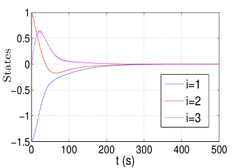
Figure 3: Convergence for unidirectional topology

For the case of bidirectional topology, we assume the topology switches between $\mathcal{G}_{4}$ and $\mathcal{G}_{5}$ in Fig. 4. The topology is $\mathcal{G}_{4}$ except at time intervals $[l^{2},l^{2}+1]$, where the topology is $\mathcal{G}_{5}$, $l=1,2,\dots$. The signed matrices associated with $\mathcal{G}_{4}$, $\mathcal{G}_{5}$ are $A_{4}=\left[\begin{smallmatrix}0.5&0&-0.5\\ 0&1&0\\ -0.5&0&0.5\end{smallmatrix}\right],~{}A_{5}=\left[\begin{smallmatrix}1&0&0\\ 0&0.5&0.5\\ 0&0.5&0.5\end{smallmatrix}\right].$ The initial states and $\mu$ are the same as previously. Fig. 5 shows the convergence of states over this bidirectional switching topology. We see that the absolute values of the agent states converge to the same limit, in accordance with the conclusion from Theorems 2.2 and 2.3. Bipartite consensus is achieved in this case.

Figure 4: Graphs $\mathcal{G}_{4}$ and $\mathcal{G}_{5}$ considered in the example.

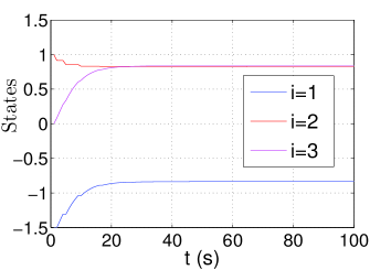
Figure 5: Convergence for bidirectional topology

5 Conclusions

In this paper, we studied the consensus problem of multi-agent systems over cooperative-antagonistic networks in a discrete-time setting. Both unidirectional and bidirectional topologies were considered. It was proven that the limits of all agent states exist and reach a consensus in absolute values if the topology is uniformly jointly strongly connected or infinitely jointly connected. We also gave an example to show that uniform quasi-strong connectedness is not sufficient to guarantee consensus in absolute values. We further proposed sufficient conditions for bipartite consensus to be achieved over networks with joint connectivity. Examples were given to explain coordination of multiple nonlinear systems with antagonistic interactions using the proposed algorithms. Future works include investigating time-delay influence and other types of antagonistic interaction models.

References

• Altafini (2012) Altafini, C., 2012. Dynamics of opinion forming in structurally balanced social networks. PloS One (7(6):e38135).
• Altafini (2013) Altafini, C., 2013. Consensus problems on networks with antagonistic interactions. IEEE Transactions on Automatic Control 58 (4), 935–946.
• Bauso et al. (2012) Bauso, D., Giarre, L., Pesenti, R., 2012. Quantized dissensus in networks of agents subject to death and duplication. IEEE Transactions on Automatic Control 57 (3), 783–788.
• Blondel et al. (2005) Blondel, V. D., Hendrickx, J. M., Olshevsky, A., Tsitsiklis, J. N., 2005. Convergence in multiagent coordination, consensus, and flocking. In: 44th IEEE Conference on Decision and Control. pp. 2996–3000.
• Cao et al. (2008a) Cao, M., Morse, A. S., Anderson, B. D. O., 2008a. Reaching a consensus in a dynamically changing environment: A graphical approach. SIAM Journal of Control and Optimization 47 (2), 575–600.
• Cao et al. (2008b) Cao, M., Morse, A. S., Anderson, B. D. O., 2008b. Reaching a consensus in a dynamically changing environment: convergence rates, measurement delays, and asynchronous events. SIAM Journal of Control and Optimization 47 (2), 601–623.
• Cartwright and Harary (1956) Cartwright, D., Harary, F., 1956. Structural balance: a generalization of Heider’s theory. Psychological review 63 (5), 277–293.
• Easley and Kleinberg (2010) Easley, D., Kleinberg, J., 2010. Networks, Crowds, and Markets: Reasoning About a Highly Connected World. Cambridge University Press, Cambridge.
• Hegselmann and Krause (2002) Hegselmann, R., Krause, U., 2002. Opinion dynamics and bounded confidence models, analysis, and simulation. Journal of Artifical Societies and Social Simulation 5 (3), 1–33.
• Hendrickx (2014) Hendrickx, J. M., December 2014. A lifting approach to models of opinion dynamics with antagonisms. In: Proceedings of the IEEE Conference on Decision and Control. Los Angeles, CA, USA, 2118–2123.
• Hendrickx and Tsitsiklis (2013) Hendrickx, J. M., Tsitsiklis, J. N., 2013. Convergence of type-symmetric and cut-balanced consensus seeking systems. IEEE Transactions Automatic Control 58 (1), 214–218.
• Jadbabaie et al. (2003) Jadbabaie, A., Lin, J., Morse, A. S., 2003. Coordination of groups of mobile autonomous agents using nearest neighbor rules. IEEE Transactions on Automatic Control 48 (6), 988–1001.
• Meng et al. (2013) Meng, Z., Lin, Z., Ren, W., 2013. Robust cooperative tracking for multiple non-identical second-order nonlinear systems. Automatica 49 (8), 2363–2372.
• Moreau (2005) Moreau, L., 2005. Stability of multi-agent systems with time-dependent communication links. IEEE Transactions on Automatic Control 50 (2), 169–182.
• Olfati-Saber et al. (2007) Olfati-Saber, R., Fax, J. A., Murray, R. M., 2007. Consensus and cooperation in networked multi-agent systems. Proceedings of the IEEE 95 (1), 215–233.
• Ren and Beard (2005) Ren, W., Beard, R. W., 2005. Consensus seeking in multiagent systems under dynamically changing interaction topologies. IEEE Transactions on Automatic Control 50 (5), 655–661.
• Shi and Hong (2009) Shi, G., Hong, Y., 2009. Global target aggregation and state agreement of nonlinear multi-agent systems with switching topologies. Automatica 45 (5), 1165–1175.
• Shi et al. (2013) Shi, G., Johansson, M., Johansson, K. H., 2013. How agreement and disagreement evolve over random dynamic networks. IEEE Journal on Selected Areas in Communications 31 (6), 1061–1071.
• Strogatz (2000) Strogatz, S. H., 2000. From Kuramoto to Crawford: exploring the onset of synchronization in populations of coupled oscillators. Physica D: Nonlinear Phenomena 143 (1-4), 1–20.
• Tsitsiklis et al. (1986) Tsitsiklis, J. N., Bertsekas, D., Athans, M., 1986. Distributed asynchronous deterministic and stochastic gradient optimization algorithms. IEEE Transactions Automatic Control 31 (9), 803–812.
• Valcher and Misra (2014) Valcher, M. E., Misra, P., 2014. On the consensus and bipartite consensus in high- order multi-agent dynamical systems with antagonistic interactions. Systems and Control Letters 66, 94–103.
• Vicsek et al. (1995) Vicsek, T., Czirok, A., Jacob, E. B., Cohen, I., Schochet, O., 1995. Novel type of phase transitions in a system of self-driven particles. Physical Review Letters 75 (6), 1226–1229.