Abstract

We construct polarized spin reversal operator (PSRO) which yields a class of representations for the $BC_{N}$ type of Weyl algebra, and subsequently use this PSRO to find out novel exactly solvable variants of the $BC_{N}$ type of spin Calogero model. The strong coupling limit of such spin Calogero models generates the $BC_{N}$ type of Polychronakos spin chains with PSRO. We derive the exact spectra of the $BC_{N}$ type of spin Calogero models with PSRO and compute the partition functions of the related spin chains by using the freezing trick. We also find out an interesting relation between the partition functions of the $BC_{N}$ type and $A_{N-1}$ type of Polychronakos spin chains. Finally, we study spectral properties like level density and distribution of spacing between consecutive energy levels for $BC_{N}$ type of Polychronakos spin chains with PSRO.

PACS No. : 02.30.Ik, 05.30.-d, 75.10.Pq, 75.10.Jm

Keywords: Exactly solvable quantum spin models, Polarized spin reversal operator, Partition function

1 Introduction

Exactly solvable one-dimensional quantum many body systems with long-range interactions have been studied intensively during last few decades [1, 2, 3, 4, 5, 6, 7, 8, 9, 10, 11, 12] and have been applied in various topics of contemporary physics as well as mathematics like generalized exclusion statistics, electric transport in mesoscopic systems, ${\cal N}=4$ super Yang-Mills theory, random matrix theory, multivariate orthogonal polynomials and Yangian quantum groups [13, 14, 15, 16, 17, 18, 19, 20, 21, 22, 23, 24, 25, 26, 27, 28, 29, 30]. Investigation of this type of quantum mechanical systems having only dynamical degrees of freedom was initiated by Calogero, who found the exact spectrum of a Hamiltonian describing particles on a line, subject to a harmonic confining potential and two-body long-range interaction inversely proportional to the square of the inter-particle distances  [1]. An exactly solvable trigonometric variant of this rational Calogero model, with particles moving on a circle and interacting through two-body potentials proportional to the inverse square of their chord distances, was subsequently studied by Sutherland [2, 3].

In a parallel development, Haldane and Shastry pioneered the study of quantum integrable spin chains with long-range interaction  [5, 6]. They found an exactly solvable quantum spin-$\frac{1}{2}~{}$chain with long-range interactions, whose ground state coincides with the $U\rightarrow\infty$ limit of Gutzwiller’s variational wave function for the Hubbard model, and yields a one-dimensional analogue of the resonating valence bond state. The lattice sites of this su($2$) Haldane–Shastry (HS) spin chain are equally spaced on a circle and all spins interact with each other through pairwise exchange interactions inversely proportional to the square of their chord distances. Integrable models possessing both spin and dynamical degrees of freedom, like su($m$) spin generalization of the Sutherland model, have been studied subsequently in the literature [31, 32, 33]. Furthermore, a close connection between the su($m$) spin generalization of the Sutherland model and the HS chain with su($m$) spin degrees of freedom has been established by using the method of ‘freezing trick’ [7, 34]. Indeed, by applying the above mentioned method, it can be shown that in the strong coupling limit the particles of the su($m$) spin Sutherland model ‘freeze’ at the equilibrium position of the scalar part of the potential, and the dynamical and spin degrees of freedom decouple from each other. Moreover, since such equilibrium positions of the particles coincide with the equally spaced lattice points of the HS spin chain, the dynamics of the decoupled spin degrees of freedom naturally leads to the Hamiltonian of the su($m$) HS model. In a similar way, application of this freezing trick to the su($m$) spin Calogero model with harmonic confining potential yields the Polychronakos spin chain (also known as Polychronakos–Frahm (PF) spin chain in the literature) with Hamiltonian given by [7, 9]

$$\mathcal{H}_{\mathrm{PF}}^{(m)}=\sum_{1\leqslant i<j\leqslant N}\frac{1+P_{ij}}{(\rho_{i}-\rho_{j})^{2}}\,,$$ (1.1)

where $\rho_{i}$ denotes the $i$-th zero of the Hermite polynomial of degree $N$ and $P_{ij}$ is the exchange operator interchanging the ‘spins’ (taking $m$ possible values) of $i$-th and $j$-th lattice sites. Thus, unlike the case of HS spin chain, the lattice sites of the PF spin chain are inhomogeneously distributed on a line. Due to the decoupling of the spin and dynamical degrees of freedom of the su($m$) spin Calogero model for large values of its coupling constant, an expression for the partition function of the su($m$) PF spin chain can be obtained by first computing the spectrum and partition function of the su($m$) spin Calogero model and then dividing such partition function by that of the spinless Calogero model [8]. Similarly, the partition function of su($m$) HS spin chain can be computed by dividing the partition function of the su($m$) spin Sutherland model at the strong coupling limit by that of the spinless Sutherland model [10].

The Hamiltonians of the above mentioned translational invariant su($m$) HS and PF spin chains, in which the strength of interaction between any two spins depends only on the difference of their site coordinates, have a close connection with the $A_{N-1}$ type of root system [4]. Variants of these spin chains associated with other root systems have also been studied in the literature and applied in the context of one dimensional physical systems with boundaries which break the translational invariance. In particular, the spectrum of an equally spaced spin-$\frac{1}{2}~{}$HS chain related to the $BC_{N}$ root system has been studied by Bernerd et al. [35]. A key feature in the Hamiltonian of this spin chain is the presence of reflection operators like $\hat{P}_{i}$ (defined on the $i$-th lattice site) satisfying the relation $\hat{P}_{i}^{2}=1\hskip-2.84526pt{\rm l}$. Since the internal space associated with each lattice site is two dimensional for this spin chain, the reflection operator yields three inequivalent representations: $\hat{P}_{i}=\pm 1\hskip-2.84526pt{\rm l}$ and $\hat{P}_{i}=\sigma^{x}$, where $\sigma^{x}$ is a Pauli matrix. For the case $\hat{P}_{i}=1\hskip-2.84526pt{\rm l}$ (or, $\hat{P}_{i}=-1\hskip-2.84526pt{\rm l}$), this spin-$\frac{1}{2}~{}$chain becomes su($2$) invariant and coincides (up to an additive constant) with a spin model with open boundary condition, which was first considered by Simons and Altshuler [36]. On the other hand, for the case $\hat{P}_{i}=\sigma^{x}$, where $\hat{P}_{i}$ can be interpreted as the spin reversal operator due to its action on the states of the $i$-th lattice site as $\hat{P}_{i}|\frac{1}{2}\rangle=|\!-\!\frac{1}{2}\rangle$, $\hat{P}_{i}|\!-\frac{1}{2}\!\rangle=|\frac{1}{2}\rangle$, this spin-$\frac{1}{2}~{}$chain associated with the $BC_{N}$ root system breaks the su($2$) symmetry.

Taking $\hat{P}_{i}$ as the spin reversal operator (denoted by $P_{i}$) for any possible value of the ‘spin’ degrees of freedom ($m\geqslant 2$), and also allowing the possibility of having unequally spaced lattice sites on a circle, the above mentioned HS spin chain associated with the $BC_{N}$ root system has been generalized by Enciso et al. [37]. By employing the freezing trick, the partition functions for this type of generalization of the HS spin chain and a similar generalization of the PF spin chain have also been calculated for all values of $m$ [37, 38]. However, to the best of our knowledge, the partition functions for the Simons-Altshuler (SA) type generalizations of HS and PF spin chains, corresponding to the cases $\hat{P}_{i}=\pm 1\hskip-2.84526pt{\rm l}$, have not been computed till now for any value of $m$. Since SA type generalizations of HS and PF spin chains would be su($m$) invariant, exact solutions of these spin chains may play an important role in describing boundary effects in physical systems which break the translational invariance but respect the internal su($m$) symmetry.

Even though $\hat{P}_{i}=\pm 1\hskip-2.84526pt{\rm l}$ and $\hat{P}_{i}=\sigma^{x}$ are the only possible inequivalent representations of the reflection operator $\hat{P}_{i}$ for the case $m=2$, in this paper it will be shown that the situation is slightly more complex for the case $m>2$. Since each inequivalent representation of the reflection operator $\hat{P}_{i}$ on a complex $m$-dimensional vector space may lead to a different type of HS or PF spin chain associated with the $BC_{N}$ root system, at present our main aim is to construct all possible inequivalent representations of $\hat{P}_{i}$ for any value of $m$ and compute the partition functions of the corresponding PF spin chains through the freezing trick. Interestingly, it will turn out that, in general a representation of $\hat{P}_{i}$ can be characterized as a polarized spin reversal operator (PSRO) which acts like the identity operator on some spin components and acts like the spin reversal operator on the rest of the spin components. In a particular limit, such PSRO coincides with the usual spin reversal operator $P_{i}$ which changes the signs of all spin components and, in the opposite limit, such PSRO yields $\hat{P}_{i}=1\hskip-2.84526pt{\rm l}$ (or, $\hat{P}_{i}=-1\hskip-2.84526pt{\rm l}$). The latter representation of $\hat{P}_{i}$ would allow us to construct a su($m$) invariant SA type generalization of the PF spin chain, which is described by the Hamiltonian

$${\mathcal{H}}^{(m,0)}=\sum_{1\leqslant i\neq j\leqslant N}\frac{y_{i}+y_{j}}{(y_{i}-y_{j})^{2}}\,(1+P_{ij})\,,$$ (1.2)

where $y_{i}$ denotes the $i$-th zero of the generalized Laguerre polynomial $L_{N}^{\beta-1}$. Hence, the lattice sites of this su($m$) invariant Hamiltonian (1.2) implicitly depend on the real positive parameter $\beta$.

The organization of this paper is as follows. In Section 2, at first we review the key role played by the $BC_{N}$ type of Weyl algebra in deriving the spectrum of the $BC_{N}$ type of spin Calogero model. Then we construct the PSRO which, along with the spin exchange operator $P_{ij}$, yields new representations of the $BC_{N}$ type of Weyl algebra in the internal space associated with $N$ number of particles or lattice sites. In Section 3, we use such PSRO to obtain novel exactly solvable variants of the $BC_{N}$ type of spin Calogero model and subsequently take the strong coupling limit of these models to construct $BC_{N}$ type of PF spin chains with PSRO. Next, we derive the exact spectrum of the $BC_{N}$ type of spin Calogero models with PSRO and also compute the partition functions of the related spin chains by using the freezing trick. In Section 4, we derive an interesting relation between the partition function of the $BC_{N}$ type of PF spin chain with PSRO and that of the $A_{N-1}$ type of PF spin chain. Then we establish a duality relation between the partition functions of the $BC_{N}$ type of anti-ferromagnetic and ferromagnetic PF spin chains with PSRO. In Section 5, we compute the ground state and the highest state energy levels corresponding to the $BC_{N}$ type of PF spin chains with PSRO. In Section 6, we study a few spectral properties of the $BC_{N}$ type of PF spin chains with PSRO, like the energy level density and nearest neighbour spacing distribution. In Section 7, we summarize our results and also mention some possible directions for future study.

2 Construction of the PSRO

Similar to the case of $A_{N-1}$ type of quantum integrable systems with long-range interaction, $BC_{N}$ type of Dunkl operators and the corresponding auxiliary operator (which is a quadratic sum of all Dunkl operators) play a central role in calculating the exact spectrum of the $BC_{N}$ type of spin Calogero model and its scalar counterpart [38]. The form of such $BC_{N}$ type of auxiliary operator is given by

$$\mathbb{H}=-\sum_{i=1}^{N}\frac{\partial^{2}}{\partial x_{i}^{2}}+a\,\sum_{i\neq j}\left[\frac{a-K_{ij}}{(x_{ij}^{-})^{2}}+\frac{a-\widetilde{K}_{ij}}{(x_{ij}^{+})^{2}}\right]+\beta a\,\sum_{i=1}^{N}\frac{\beta a-K_{i}}{x_{i}^{2}}+\frac{a^{2}}{4}\,r^{2}\,,$$ (2.1)

where $a>\frac{1}{2},~{}\beta>0$ are some real coupling constants and the notations $x_{ij}^{-}\equiv x_{i}-x_{j}$, $x_{ij}^{+}\equiv x_{i}+x_{j}$ and $r^{2}\equiv\sum_{i=1}^{N}x_{i}^{2}$ are used. Moreover, $K_{ij}$ and $K_{i}$ are coordinate permutation and sign reversing operators, defined by

$$(K_{ij}f)(x_{1},\dots,x_{i},\dots,x_{j},\dots,x_{N})=f(x_{1},\dots,x_{j},\dots,x_{i},\dots,x_{N})\,,$$ (2.2a)

$$(K_{i}f)(x_{1},\dots,x_{i},\dots,x_{N})=f(x_{1},\dots,-x_{i},\dots,x_{N})\,,$$ (2.2b)

and $\widetilde{K}_{ij}=K_{i}K_{j}K_{ij}$. Thus the operators $K_{ij}$, $K_{i}$ and $\mathbb{H}$ act on the functions of the coordinate space, which is denoted by $C^{\infty}(\mathbb{R}^{N})$ . By using Eq. (2.2), it is easy to check that $K_{ij}$ and $K_{i}$ give a realization of the $BC_{N}$ type of Weyl algebra generated by $\mathcal{W}_{ij}$ and $\mathcal{W}_{i}\,$:

$$\mathcal{W}_{ij}^{2}=1\hskip-2.84526pt{\rm l}\,,~{}~{}~{}~{}\mathcal{W}_{ij}\mathcal{W}_{jk}=\mathcal{W}_{ik}\mathcal{W}_{ij}=\mathcal{W}_{jk}\mathcal{W}_{ik}\,,~{}~{}~{}~{}\mathcal{W}_{ij}\mathcal{W}_{kl}=\mathcal{W}_{kl}\mathcal{W}_{ij}\,,$$ (2.3a)

$$\mathcal{W}_{i}^{2}=1\hskip-2.84526pt{\rm l}\,,~{}~{}~{}~{}\mathcal{W}_{i}\mathcal{W}_{j}=\mathcal{W}_{j}\mathcal{W}_{i}\,,~{}~{}~{}~{}\mathcal{W}_{ij}\mathcal{W}_{k}=\mathcal{W}_{k}\mathcal{W}_{ij}\,,~{}~{}~{}~{}\mathcal{W}_{ij}\mathcal{W}_{j}=\mathcal{W}_{i}\mathcal{W}_{ij}\,.$$ (2.3b)

The Hamiltonian of the $BC_{N}$ type of spin Calogero model, as considered in Ref. [38], is quite similar in form to that of the auxiliary operator (2.1). However, this Hamiltonian acts not only on the functions of the coordinate space, but on a direct product space like $C^{\infty}(\mathbb{R}^{N})\otimes\mathcal{S}$ , where

$$\mathcal{S}\equiv\underbrace{\mathcal{C}_{m}\otimes\mathcal{C}_{m}\cdots\otimes\mathcal{C}_{m}}_{N}\,,$$ (2.4)

with $\mathcal{C}_{m}$ denoting the $m$-dimensional complex vector space associated with each particle. In terms of orthonormal basis vectors, the total spin space $\mathcal{S}$ may be expressed as

$$\mathcal{S}=\Big{\langle}|s_{1},\cdots,s_{N}\rangle^{*}~{}\Big{|}s_{i}\in\{-M,-M+1,\cdots,M\};~{}M=\frac{m-1}{2}\Big{\rangle}\,.$$ (2.5)

The spin exchange operator $P_{ij}$ and the spin reversal operator $P_{i}$ are defined on the space $\mathcal{S}$ as

$$P_{ij}|s_{1}\,,\cdots,s_{i}\,,\cdots,s_{j}\,,\cdots,s_{N}\rangle^{*}=|s_{1}\,,\cdots,s_{j}\,,\cdots,s_{i}\,,\cdots,s_{N}\rangle^{*}$$ (2.6a)

$$P_{i}|s_{1}\,,\cdots,s_{i}\,,\cdots,s_{N}\rangle^{*}=|s_{1}\,,\cdots,-s_{i}\,,\cdots,s_{N}\rangle^{*}\,.$$ (2.6b)

It is easy to check that, similar to the case of $K_{ij}$ and $K_{i}$, $P_{ij}$ and $P_{i}$ also give a realization of the $BC_{N}$ type of Weyl algebra (2.3). By using the operators $P_{ij}$ and $P_{i}$, one can define the Hamiltonian of the $BC_{N}$ type of spin Calogero model as [38]

$$H^{(m)}=-\sum_{i=1}^{N}\frac{\partial^{2}}{\partial x_{i}^{2}}+a\sum_{i\neq j}\left[\frac{a+P_{ij}}{(x_{ij}^{-})^{2}}+\frac{a+\widetilde{P}_{ij}}{(x_{ij}^{+})^{2}}\right]+\beta a\sum_{i=1}^{N}\frac{\beta a-\epsilon P_{i}}{x_{i}^{2}}+\frac{a^{2}}{4}r^{2}\,,$$ (2.7)

where $\epsilon=\pm 1$ and $\widetilde{P}_{ij}\equiv P_{i}P_{j}P_{ij}$. Note that the Hamiltonian (2.7) of $BC_{N}$ spin Calogero model can be reproduced from the auxiliary operator (2.1) through simple substitutions like

$$H^{(m)}=\mathbb{H}\big{|}_{K_{ij}\rightarrow-P_{ij},\,K_{i}\rightarrow\epsilon P_{i}}\,.$$ (2.8)

Consequently, the Hilbert space and the spectrum of $H^{(m)}$ can be obtained from those of $\mathbb{H}$ by applying a projector $\Lambda$ which satisfies the relations [38]

$$K_{ij}P_{ij}\Lambda=\Lambda K_{ij}P_{ij}=-\Lambda$$ (2.9a)

$$K_{i}P_{i}\Lambda=\Lambda K_{i}\,P_{i}=\epsilon\Lambda\,.$$ (2.9b)

For constructing the projector $\Lambda$, it is important to observe that both of the two sets of operators given by $K_{ij},~{}K_{i}$ and $P_{ij},~{}P_{i}$ yield realizations of the $BC_{N}$ type of Weyl algebra (2.3) on the spaces $C^{\infty}(\mathbb{R}^{N})$ and $\mathcal{S}$ respectively. Hence, it is possible to define another set of operators like $\Pi_{ij}=K_{ij}P_{ij},~{}\Pi_{i}=K_{i}P_{i}$, which will yield a realization of the $BC_{N}$ type of Weyl algebra (2.3) on the space $C^{\infty}(\mathbb{R}^{N})\otimes\mathcal{S}$ . Let us now define an operator $\Lambda_{0}$ on the space $C^{\infty}(\mathbb{R}^{N})\otimes\mathcal{S}$ as

$$\Lambda_{0}=\frac{1}{N!}\sum_{i=1}^{N!}\,\varepsilon_{l}\,\mathcal{P}_{l}\,,$$ (2.10)

where $\mathcal{P}_{l}$ denotes an element of the realization of the permutation group generated by the operators $\Pi_{ij}$ and $\varepsilon_{l}$ is the signature of $\mathcal{P}_{l}$. For example, corresponding to the simplest $N=2$ and $N=3$ cases, $\Lambda_{0}$ is given by

$$N=2:~{}~{}~{}~{}~{}~{}\Lambda_{0}=\frac{1}{2}\left(1-\Pi_{12}\right)\,,$$

$$N=3:~{}~{}~{}~{}~{}~{}\Lambda_{0}=\frac{1}{6}\left(1-\Pi_{12}-\Pi_{13}-\Pi_{23}+\Pi_{12}\Pi_{13}+\Pi_{12}\Pi_{23}\right)\,.$$

It is easy to show that $\Lambda_{0}$ in Eq. (2.10) satisfies the relations

$$\Lambda_{0}^{2}=\Lambda_{0},~{}~{}K_{ij}P_{ij}\Lambda_{0}=\Lambda_{0}K_{ij}P_{ij}=-\Lambda_{0}\,.$$

Hence $\Lambda_{0}$ acts as an antisymmetriser with respect to the simultaneous interchange of the coordinate and the spin degrees of freedom. With the help of this $\Lambda_{0}$, it is possible to finally construct the projector $\Lambda$ as [39]

$$\Lambda=\frac{1}{2^{N}}\left(\prod_{j=1}^{N}\left(1+\epsilon\,\Pi_{j}\right)\right)\Lambda_{0}\,.$$ (2.11)

Using the fact that $\Pi_{ij}$ and $\Pi_{i}$ yield a realization of the $BC_{N}$ type of Weyl algebra (2.3), one can easily verify that the projector $\Lambda$ satisfies the relations (2.9). Hence, with the help of the projector given in (2.11), it is possible to compute the spectrum of $H^{(m)}$ from the known spectrum of the auxiliary operator.

Even though the projector (2.11) is constructed for a particular representation of the $BC_{N}$ type of Weyl algebra (2.3), such a projector can also be written in an abstract algebraic form [40]. Therefore, if we can modify the action of $P_{i}$ given in Eq. (2.6b) so that, along with $P_{ij}$ in (2.6a), this modified version of $P_{i}$ yields an inequivalent representation of the $BC_{N}$ type of Weyl algebra (2.3), then it would be possible to explicitly construct the corresponding projector in exactly same way. Consequently, such modified version of $P_{i}$ would lead to a new $BC_{N}$ type of spin Calogero model whose spectrum can be computed by using the method of projector. For the purpose of finding out modified versions of $P_{i}$ which may give inequivalent representations of the $BC_{N}$ type of Weyl algebra, at first we notice that the spin reversal operator $P_{i}$ in Eq. (2.6b) acts nontrivially only on the $i$-th spin space. Hence, this $P_{i}$ can also be written in the form

$$\begin{array}[]{clc}{P_{i}=1\hskip-2.84526pt{\rm l}\otimes\cdots\otimes 1\hskip-2.84526pt{\rm l}}&{\otimes~{}~{}P~{}~{}\otimes}&{\!\!1\hskip-2.84526pt{\rm l}\otimes\cdots\otimes 1\hskip-2.84526pt{\rm l}}\,,\\ {}\hfil&{\text{i-th place}}&{}\hfil\end{array}$$ (2.12)

where $P$ acts on $\mathcal{C}^{m}$ as

$$P|s_{i}\rangle^{*}=|-s_{i}\rangle^{*}\,.$$ (2.13)

In analogy with this case, we assume that all modified versions of $P_{i}$ act nontrivially only on the $i$-th spin space. Due to the relation $\mathcal{W}_{i}^{2}=1\hskip-2.84526pt{\rm l}$ within Eq. (2.3b), such modified versions of $P_{i}$ can be treated as involutions on the $i$-th spin space. It is known that the Hamiltonian of the $BC_{N}$ type of spin Calogero model, with reflection operators formally defined as involutions on the corresponding spin spaces, yields a quantum integrable system with mutually commuting conserved quantities [41]. Consequently, the spin Calogero models which we shall construct in the next section by using modified versions of $P_{i}$ would also represent quantum integrable systems.

For the purpose of explicitly finding out all possible modified versions of $P_{i}$, which act as involutions on the $i$-th spin space and also satisfy the $BC_{N}$ type of Weyl algebra (2.3), let us arbitrarily partition $m$ into two parts as $m=m_{1}+m_{2}$, where $m_{1}\geqslant m_{2}\geqslant 0$. Evidently, the internal space $\mathcal{C}_{m}$ associated with the $i$-th particle can always be written as a direct sum of any two orthogonal subspaces of dimension $m_{1}-m_{2}$ and $2m_{2}$ respectively:

$$\mathcal{C}_{m}=\mathcal{C}_{m_{1}-m_{2}}\oplus\mathcal{C}_{2m_{2}}\,,$$ (2.14)

where $\mathcal{C}_{m_{1}-m_{2}}$ and $\mathcal{C}_{2m_{2}}$ are defined in terms of orthonormal basis vectors as

$$\mathcal{C}_{m_{1}-m_{2}}=\Big{\langle}|\alpha\rangle^{\prime}~{}\Big{|}\,\alpha\in\{1,2,\cdots,m_{1}-m_{2}\}\Big{\rangle}\,,~{}\mathcal{C}_{2m_{2}}=\Big{\langle}|\beta\rangle^{\prime\prime}~{}\Big{|}\,\beta\in\{1,2,\cdots,2m_{2}\}\Big{\rangle}\,.$$ (2.15)

In analogy with Eq. (2.12), we propose a modification of $P_{i}$ in the form

$$\begin{array}[]{clc}{P_{i}=1\hskip-2.84526pt{\rm l}\otimes\cdots\otimes 1\hskip-2.84526pt{\rm l}}&{\otimes~{}~{}P^{(m_{1},m_{2})}~{}~{}\otimes}&{\!\!1\hskip-2.84526pt{\rm l}\otimes\cdots\otimes 1\hskip-2.84526pt{\rm l}}\,,\\ {}\hfil&{\text{~{}~{}~{}~{}i-th place}}&{}\hfil\end{array}$$ (2.16)

where $P^{(m_{1},m_{2})}$ acts in a rather different way on the two subspaces $\mathcal{C}_{m_{1}-m_{2}}$ and $\mathcal{C}_{2m_{2}}$ of the space $\mathcal{C}_{m}$. More precisely, $P^{(m_{1},m_{2})}$ acts like an identity operator on the space $\mathcal{C}_{m_{1}-m_{2}}$ and acts like a spin reversal operator on the even dimensional space $\mathcal{C}_{2m_{2}}$. Thus, the action of $P^{(m_{1},m_{2})}$ on the basis vectors of $\mathcal{C}_{m_{1}-m_{2}}$ is given by

$$P^{(m_{1},m_{2})}|\alpha\rangle^{\prime}=|\alpha\rangle^{\prime}\,.$$ (2.17)

Moreover, in analogy with Eq. (2.13), the action of $P^{(m_{1},m_{2})}$ on the first basis vector of $\mathcal{C}_{2m_{2}}$ would give the last basis vector of this space, on the second basis vector would give the last but one basis vector, and so on. Hence, in general, the action of $P^{(m_{1},m_{2})}$ on the basis vectors of $\mathcal{C}_{2m_{2}}$ may be written as

$$P^{(m_{1},m_{2})}|\beta\rangle^{\prime\prime}=|2m_{2}+1-\beta\rangle^{\prime\prime}\,.$$ (2.18)

Since $P^{(m_{1},m_{2})}$ acts like a spin reversal operator only on a subspace of $\mathcal{C}_{m}$, and acts trivially on the complementary subspace, it is natural to call $P_{i}^{(m_{1},m_{2})}$ as a PSRO associated with the $i$-th particle. Note that the relation $\left(P^{(m_{1},m_{2})}\right)^{2}=1\hskip-2.84526pt{\rm l}$ is satisfied for both of the spaces $\mathcal{C}_{m_{1}-m_{2}}$ and $\mathcal{C}_{2m_{2}}$. For the purpose of representing $P^{(m_{1},m_{2})}$ in a more convenient form, let us take another set of orthonormal basis vectors of $\mathcal{C}_{2m_{2}}$ as

$$|\beta\rangle_{\pm}=\frac{1}{\sqrt{2}}\,\big{(}\,|\beta\rangle^{\prime\prime}\pm|2m_{2}+1-\beta\rangle^{\prime\prime}\,\big{)}\,,$$ (2.19)

where $\beta\in\{1,2,\ldots,m_{2}\}$. By using Eq. (2.18), it is easy to check that

$$P^{(m_{1},m_{2})}|\beta\rangle_{\pm}=\pm\,|\beta\rangle_{\pm}\,.$$ (2.20)

Due to Eq. (2.14), we can choose an orthonormal set of basis vectors for the space $\mathcal{C}_{m}$ as

$$\mathcal{C}_{m}=\Big{\langle}\,|s\rangle\,\Big{|}\,s\in\{1,2,\cdots,m_{1}+m_{2}\}\,\Big{\rangle}\,,$$ (2.21)

where $|s\rangle=|\alpha\rangle^{\prime}$ with $\alpha=s$ for $s\in\{1,2,\cdots,m_{1}-m_{2}\}$, $|s\rangle=|\beta\rangle_{+}$ with $\beta=s-m_{1}+m_{2}$ for $s\in\{m_{1}-m_{2}+1,m_{1}-m_{2}+2,\cdots,m_{1}\}$ and $|s\rangle=|\beta\rangle_{-}$ with $\beta=s-m_{1}$ for $s\in\{m_{1}+1,m_{1}+2,\cdots,m_{1}+m_{2}\}$. Using Eqs. (2.17) and (2.20), it is easy to show that $P^{(m_{1},m_{2})}$ acts as a diagonal matrix on the basis vectors (2.21) of $\mathcal{C}_{m}$:

$$P^{(m_{1},m_{2})}=\begin{pmatrix}1&\\ &\ddots&\\ &&1&\\ &&&-1&\\ &&&&\ddots&\\ &&&&&-1&\\ \end{pmatrix}\,,$$ (2.22)

where there are $m_{1}$ number of 1’s and $m_{2}$ number of -1’s along the main diagonal. Combining Eqs. (2.4) and (2.21), we express the total spin space $\mathcal{S}$ through a set of orthonormal basis vectors as

$$\mathcal{S}=\Big{\langle}|s_{1},\cdots,s_{N}\rangle~{}\Big{|}s_{i}\in\{1,2,\cdots,m\}\Big{\rangle}\,.$$ (2.23)

Due to Eqs. (2.16) and (2.22), $P_{i}^{(m_{1},m_{2})}$ acts on these basis vectors as

$$P_{i}^{(m_{1},m_{2})}|s_{1},\cdots,s_{i},\cdots,s_{N}\rangle=(-1)^{f(s_{i})}|s_{1},\cdots,s_{i},\cdots,s_{N}\rangle,$$ (2.24)

where

$$f(s_{i})=\left\{\begin{array}[]{ll}0,&\mbox{~{}for $s_{i}\in\{1,2,\ldots,m_{1}\}$, }\\ 1,&\mbox{~{}for $s_{i}\in\{m_{1}+1,\ldots,m_{1}+m_{2}\}$. }\end{array}\right.$$

In analogy with Eq. (2.6a), we define the action of $P_{ij}$ on the basis vectors (2.23) as

$$P_{ij}|s_{1}\,,\cdots,s_{i}\,,\cdots,s_{j}\,,\cdots,s_{N}\rangle=|s_{1}\,,\cdots,s_{j}\,,\cdots,s_{i}\,,\cdots,s_{N}\rangle\,.$$ (2.25)

Using Eqs. (2.24) and (2.25), one can easily check that $P_{i}^{(m_{1},m_{2})}$ and $P_{ij}$ yield a realization of the $BC_{N}$ type of Weyl algebra (2.3). In this context it may be recalled that, while constructing $P_{i}^{(m_{1},m_{2})}$ as a PSRO, we have previously assumed that $m_{1}\geqslant m_{2}$. However, this condition is really not necessary for showing that $P_{i}^{(m_{1},m_{2})}$ and $P_{ij}$ yield a realization of the $BC_{N}$ type of Weyl algebra. Therefore, in the rest of this article we shall take Eq. (2.24), with any possible values of $m_{1}$ and $m_{2}$ satisfying the condition $m_{1}+m_{2}=m$, as the definition of PSRO. Since the trace of $P_{i}^{(m_{1},m_{2})}$ in Eq. (2.24) is given by

$$\operatorname{tr}P_{i}^{(m_{1},m_{2})}=m^{N-1}(m_{1}-m_{2})\,,$$ (2.26)

it is evident that, for any given value of $m$, $P_{i}^{(m_{1},m_{2})}$ with each distinct set of values for $m_{1}$ and $m_{2}$ would lead to an inequivalent realization of the $BC_{N}$ type of Weyl algebra. In the next section, we shall use such PSRO to obtain new exactly solvable variants of the $BC_{N}$ type of spin Calogero model (2.7) and the related PF spin chain. It may be observed that the trace of the spin reversal operator $P_{i}$ in Eq. (2.6b) is given by

$$\operatorname{tr}P_{i}=m^{N-1}\times\left(m\operatorname{mod}2\right)\,.$$ (2.27)

Comparing Eq. (2.26) with Eq. (2.27) we find that, the trace of $P_{i}^{(m_{1},m_{2})}$ coincides with that of $\epsilon P_{i}$ in the special case $m_{1}=m_{2}$ ($m_{1}=m_{2}+\epsilon$) for even (odd) values of $m$. Since both of the operators $P_{i}^{(m_{1},m_{2})}$ and $\epsilon P_{i}$ can only have eigenvalues $\pm 1$, these two operators yield exactly same set of eigenvalues and lead to equivalent representations of the $BC_{N}$ type of Weyl algebra for the above mentioned choice of $m_{1}$ and $m_{2}$. It may also be noted that, for the special case $m_{1}=m,~{}m_{2}=0$, $P_{i}^{(m_{1},m_{2})}$ in Eq. (2.24) reduces to the trivial identity operator.

3 Spectra and partition functions of $BC_{N}$ type models with PSRO

In this section, we shall use the PSRO for obtaining new variants of the $BC_{N}$ type of spin Calogero model (2.7) and subsequently take the strong coupling limit of such spin Calogero models to construct the corresponding $BC_{N}$ type of PF spin chains. Next, by using the method of projector which has been discussed in the previous section, we shall find out the exact spectrum of $BC_{N}$ type of spin Calogero models with PSRO. Finally we shall compute the partition functions of the $BC_{N}$ type of PF spin chains with PSRO by using the freezing trick.

Substituting $\epsilon P_{i}$ by $P_{i}^{(m_{1},m_{2})}$ in the Hamiltonian (2.7), we obtain the Hamiltonians of the $BC_{N}$ type of spin Calogero models with PSRO as

$$H^{(m_{1},m_{2})}=-\sum_{i=1}^{N}\frac{\partial^{2}}{\partial x_{i}^{2}}+a\sum_{i\neq j}\left[\frac{a+P_{ij}}{(x_{ij}^{-})^{2}}+\frac{a+\widetilde{P}_{ij}^{(m_{1},m_{2})}}{(x_{ij}^{+})^{2}}\right]+\beta a\sum_{i=1}^{N}\frac{\beta a-P_{i}^{(m_{1},m_{2})}}{x_{i}^{2}}+\frac{a^{2}}{4}r^{2},$$ (3.1)

where $\widetilde{P}_{ij}^{(m_{1},m_{2})}\equiv P_{i}^{(m_{1},m_{2})}P_{j}^{(m_{1},m_{2})}P_{ij}$. Since $P_{i}^{(m_{1},m_{2})}$ and $\epsilon P_{i}$ yield equivalent representations of the $BC_{N}$ type of Weyl algebra in the special case $m_{1}=m_{2}$ ($m_{1}=m_{2}+\epsilon$) for even (odd) values of $m$, $H^{(m_{1},m_{2})}$ (3.1) would reduce to $H^{(m)}$ (2.7) after an appropriate similarity transformation in this special case. In another special case given by $m_{1}=m,~{}m_{2}=0$, where $P_{i}^{(m_{1},m_{2})}$ reduces to the identity operator, $H^{(m_{1},m_{2})}$ (3.1) yields an SA type extension of spin Calogero model given by

$$H^{(m,0)}=-\sum_{i=1}^{N}\frac{\partial^{2}}{\partial x_{i}^{2}}+a\sum_{i\neq j}(a+P_{ij})\left[\frac{1}{(x_{ij}^{-})^{2}}+\frac{1}{(x_{ij}^{+})^{2}}\right]+\beta a(\beta a-1)\sum_{i=1}^{N}\frac{1}{x_{i}^{2}}+\frac{a^{2}}{4}r^{2}\,.$$ (3.2)

It may be noted that, the above Hamiltonian has been obtained earlier by using an auxiliary operator, which was constructed through a combination of several $A_{N-1}$ type of Dunkl operators [42]. However, at present we have obtained this Hamiltonian (3.2) as a special case of (3.1), which will be shown to be related to the $B_{N}$ type of Dunkl operators. Thus the Hamiltonian $H^{(m,0)}$ is surprisingly related to both $A_{N-1}$ and $B_{N}$ types of Dunkl operators.

Since the potentials of the Hamiltonian $H^{(m_{1},m_{2})}$ (3.1) become singular in the limits $x_{i}\pm x_{j}\to 0$ and $x_{i}\to 0$, the configuration space of this Hamiltonian can be taken as one of the maximal open subsets of $\mathbb{R}^{N}$ on which linear functionals $x_{i}\pm x_{j}$ and $x_{i}$ have constant signs, i.e., one of the Weyl chambers of the $BC_{N}$ root system. Let us choose this configuration space as the principal Weyl chamber given by

$$C=\{\mathbf{x}\equiv(x_{1},x_{2},\cdots,x_{N}):~{}0<x_{1}<x_{2}<\ldots<x_{N}\}\,.$$ (3.3)

Note that this configuration space does not depend on the values of $m_{1}$ and $m_{2}$, and coincides with the configuration space of $H^{(m)}$ [38]. The Hamiltonian of the $BC_{N}$ type of PF spin chains with PSRO can be obtained from the Hamiltonian (3.1) in the limit $a\to\infty$ by means of the freezing trick. To this end, we express $H^{(m_{1},m_{2})}$ (3.1) in powers of the coupling constant $a$ as

$$H^{(m_{1},m_{2})}=-\sum_{i=1}^{N}\frac{\partial^{2}}{\partial x_{i}^{2}}+a^{2}\,U+O(a)\,,$$ (3.4)

with

$$U(x)=\sum_{i\neq j}\left[\frac{1}{(x_{ij}^{-})^{2}}+\frac{1}{(x_{ij}^{+})^{2}}\right]+\beta^{2}\sum_{i=1}^{N}\frac{1}{x_{i}^{2}}+\frac{r^{2}}{4}.$$ (3.5)

As the coefficient of $a^{2}$ order term in (3.4) dominates in the limit $a\to\infty$, the particles of the spin dynamical model (3.1) concentrate at the coordinates $\xi_{i}$ of the minimum $\boldsymbol{\xi}$ of the potential $U$ in $C$. Since the Hamiltonian (3.1) can be written in the form

$$H^{(m_{1},m_{2})}=H_{sc}+a\,\mathfrak{H}^{(m_{1},m_{2})}\,,$$ (3.6)

where $H_{sc}$ is the scalar (spinless) Calogero model of $B_{N}$ type given by

$$H_{sc}=-\sum_{i=1}^{N}\frac{\partial^{2}}{\partial x_{i}^{2}}+a(a-1)\sum_{i\neq j}\bigg{[}\frac{1}{(x_{ij}^{-})^{2}}+\frac{1}{(x_{ij}^{+})^{2}}\bigg{]}+\sum_{i}\frac{a\beta(a\beta-1)}{x_{i}^{2}}+\frac{a^{2}}{4}\,r^{2}\,,$$ (3.7)

and

$$\mathfrak{H}^{(m_{1},m_{2})}=\sum_{i\neq j}\left[\frac{1+P_{ij}}{(x_{i}-x_{j})^{2}}+\frac{1+\widetilde{P}_{ij}^{(m_{1},m_{2})}}{(x_{i}+x_{j})^{2}}\right]+\beta\sum_{i=1}^{N}\frac{1-P_{i}^{(m_{1},m_{2})}}{x_{i}^{2}}\,,$$ (3.8)

it follows that the dynamical and internal degrees of freedom of $H^{(m_{1},m_{2})}$ decouple from each other in the limit $a\to\infty$. Moreover, in this freezing limit, the internal degrees of freedom of $H^{(m_{1},m_{2})}$ are governed by the Hamiltonian $\mathcal{H}^{(m_{1},m_{2})}=\mathfrak{H}^{(m_{1},m_{2})}|_{\mathbf{x}\to\boldsymbol{\xi}}$, which is explicitly given by

$$\mathcal{H}^{(m_{1},m_{2})}=\sum_{i\neq j}\left[\frac{1+P_{ij}}{(\xi_{i}-\xi_{j})^{2}}+\frac{1+\widetilde{P}_{ij}^{(m_{1},m_{2})}}{(\xi_{i}+\xi_{j})^{2}}\right]+\beta\sum_{i=1}^{N}\frac{1-P_{i}^{(m_{1},m_{2})}}{\xi_{i}^{2}}\,.$$ (3.9)

The operator $\mathcal{H}^{(m_{1},m_{2})}$ in the above equation represents the Hamiltonian of the $BC_{N}$ type of PF spin chain with PSRO, whose lattice sites $\xi_{i}$ are the coordinates of the unique minimum $\boldsymbol{\xi}$ of the potential $U$ (3.5) within the configuration space $C$ (3.3). The uniqueness of such minimum was established in Ref. [43] by expressing the potential $U$ in terms of the logarithm of the ground state wave function of the scaler Calogero model (3.7). The ground state wave function of this scaler Calogero model takes the form

$$\mu({\bf x})=e^{-\frac{a}{4}r^{2}}~{}\prod_{i}|x_{i}|^{\beta a}~{}\prod_{i<j}|x_{i}^{2}-x_{j}^{2}|^{a},$$ (3.10)

and the corresponding ground state energy is given by

$$E_{0}=Na\Big{(}\beta a+a(N-1)+\frac{1}{2}\Big{)}\,.$$ (3.11)

Since the sites $\xi_{i}$ coincide with the coordinates of the (unique) critical point of $\log\mu({\bf x})$ in $C$, they can be determined through the set of relations [43, 38]

$$\sum_{\stackrel{{\scriptstyle j=1}}{{(j\neq i)}}}^{N}\,\frac{2y_{i}}{y_{i}-y_{j}}\,=\,y_{i}-\beta\,,$$ (3.12)

where $\xi_{i}=\sqrt{2y_{i}}$ and $y_{i}$’s satisfying (3.12) represent the zero points of the generalized Laguerre polynomial $L_{N}^{\beta-1}$. Due to the presence of the operator $P_{i}^{(m_{1},m_{2})}$, the Hamiltonian (3.9) is not su($m$) invariant in general. However, in the special case given by $m_{1}=m,~{}m_{2}=0$, $\mathcal{H}^{(m_{1},m_{2})}$ in (3.9) reduces to the su($m$) invariant SA type generalization of the PF spin chain (1.2), whose partition function has not been computed till now. On the other hand, using a similarity transformation in the special case given by $m_{1}=m_{2}$ ($m_{1}=m_{2}+\epsilon$) for even (odd) values of $m$, $\mathcal{H}^{(m_{1},m_{2})}$ can be reduced to the Hamiltonian

$$\mathcal{H}^{(m)}=\sum_{i\neq j}\left[\frac{1+P_{ij}}{(\xi_{i}-\xi_{j})^{2}}+\frac{1+\widetilde{P}_{ij}}{(\xi_{i}+\xi_{j})^{2}}\right]+\beta\sum_{i=1}^{N}\frac{1-\epsilon P_{i}}{\xi_{i}^{2}}\,,$$ (3.13)

whose partition function has been computed earlier by using the freezing trick [38].

We have already seen that the spin and dynamical degrees of freedom of the Hamiltonian (3.1) decouple in the freezing limit $a\to\infty$. Hence, due to Eq. (3.6), eigenvalues of ${H}^{(m_{1},m_{2})}$ are approximately given by

$$E_{ij}\simeq E_{i}^{sc}+a\,\mathcal{E}_{j}\,,$$ (3.14)

where $E_{i}^{sc}$ and $\mathcal{E}_{j}$ are two arbitrary eigenvalues of $H_{sc}$ and $\mathcal{H}^{(m_{1},m_{2})}$ respectively. By using the asymptotic relation (3.14), one can easily derive an exact formula for the partition function $\mathcal{Z}_{N}^{(m_{1},m_{2})}(T)$ of the spin chain (3.9) as

$$\mathcal{Z}_{N}^{(m_{1},m_{2})}(T)=\lim_{a\rightarrow\infty}\frac{Z^{(m_{1},m_{2})}_{N}(aT)}{Z_{N}(aT)}\,,$$ (3.15)

where $Z_{N}^{(m_{1},m_{2})}(aT)$ denotes the partition function for the spin dynamical model (3.1) and $Z_{N}(aT)$ denotes that of the scalar model (3.7). Therefore, we can evaluate the partition function $\mathcal{Z}_{N}^{(m_{1},m_{2})}(T)$ of the spin chain (3.9) by computing first the spectra and partition functions of the Hamiltonians $H^{(m_{1},m_{2})}$ and $H_{sc}$. To this end, we shall follow the approach of Ref. [38], where the auxiliary operator (2.1) and related Dunkl operators have played a key role. The form of rational Dunkl operators of $BC_{N}$ type are given by

$$J_{i}^{-}=\frac{\partial}{\partial x_{i}}+a\sum_{j\neq i}\left[\frac{1}{x_{ij}^{-}}(1-K_{ij})\,+\frac{1}{x_{ij}^{+}}(1-\widetilde{K}_{ij})\right]+\beta a\,\frac{1}{x_{i}}(1-K_{i})\,,$$ (3.16)

where $i\in\{1,2,\dots,N\}$. The auxiliary operator (2.1) can be written through these Dunkl operators as

$$\mathbb{H}=\mu(\mathbf{x})\left[-\sum_{i}\big{(}J_{i}^{-}\big{)}^{2}+a\sum_{i}x_{i}\frac{\partial}{\partial x_{i}}+E_{0}\right]\mu^{-1}(\mathbf{x})\,.$$ (3.17)

Evidently, the Dunkl operators (3.16) map any monomial $\prod_{i}x_{i}^{n_{i}}$ into a polynomial of total degree $n_{1}+n_{2}+\cdots+n_{N}-1$. Therefore, if we consider a Hilbert space having a set of basis vectors like

$$\phi_{\bf{n}}({\bf x})=\mu({\bf x})\prod_{i}x_{i}^{n_{i}},$$ (3.18)

with $n_{i}$’s being arbitrary non-negative integers, and partially order these basis vectors according to the total degree $|\mathbf{n}|\equiv n_{1}+n_{2}+\cdots+n_{N}$, then it follows from Eq. (3.17) that the operator $\mathbb{H}$ would become an upper triangular matrix in the aforesaid nonorthonormal basis. More precisely,

$$\mathbb{H}\phi_{\bf{n}}({\bf x})=E_{\mathbf{n}}\phi_{\bf{n}}({\bf x})+\sum_{|{\bf m}|<|{\bf n}|}c_{{\bf m}{\bf n}}\,\phi_{\bf m}({\bf x})\,,$$ (3.19)

where

$$E_{\bf n}=a|{\bf n}|+E_{0}\,,$$ (3.20)

and the coefficients $c_{{\bf m}{\bf n}}$ are real constants. Since the diagonal elements of any upper triangular matrix coincide with its eigenvalues, the spectrum of $\mathbb{H}$ is given by Eq. (3.20) where $n_{i}$’s can be taken as arbitrary non-negative integers.

Note that the Hamiltonians of both scalar Calogero model (3.7) and the spin Calogero model with PSRO (3.1) may be obtained from the auxiliary operator (2.1) through formal substitutions like

$$H_{sc}=\mathbb{H}|_{K_{ij},\,K_{i}\rightarrow 1}\,,$$ (3.21a)

$$H^{(m_{1},m_{2})}=\mathbb{H}|_{K_{ij}\rightarrow-P_{ij}^{(m_{1},m_{2})},\,K_{i}\rightarrow P_{i}^{(m_{1},m_{2})}}\,.$$ (3.21b)

Consequently, it would be possible to compute the spectra of these Hamiltonians from the known spectrum of the auxiliary operator with the help of appropriate projectors. For the purpose of obtaining the spectrum of $H_{sc}$ (3.7), one considers scalar functions of the form [38]

$$\psi_{\mathbf{n}}(\mathbf{x})=\Lambda_{sc}\,\phi_{\bf{n}}({\bf x})\,,$$ (3.22)

where $\Lambda_{sc}$ is the symmetriser with respect to both permutations and sign reversals, i.e., it satisfies the relations given by

$$K_{ij}\Lambda_{sc}=\Lambda_{sc}K_{ij}=\Lambda_{sc}\,,~{}~{}~{}~{}K_{i}\Lambda_{sc}=\Lambda_{sc}K_{i}=\Lambda_{sc}\,.$$ (3.23)

By using these relations, it can be shown that the functions (3.22) form a (nonorthonormal) basis of the Hilbert space of $H_{sc}$, provided that $n_{i}=2k_{i}$ are even integers and $k_{1}\geqslant k_{2}\geqslant\cdots\geqslant k_{N}$. As before, one can define a partial ordering among these basis vectors by comparing their degree. Due to Eqs. (3.21a) and (3.23), it follows that $H_{sc}$ (3.7) can be written as an upper triangular matrix with diagonal elements $E^{sc}_{\bf n}$ also given by the right hand side of Eq. (3.20). Thus one obtains the exact partition function of the $BC_{N}$ type of scalar Calogero model (3.7) as [38]

$$Z_{N}(aT)=\sum_{k_{1}\geqslant k_{2}\geqslant\dots\geqslant\,k_{N}\geqslant\,0}q^{2|{\bf k}|+\tilde{E}_{0}}=\frac{q^{\tilde{E}_{0}}}{\prod\limits_{j=1}^{N}(1-q^{2j})}\,,$$ (3.24)

where $q=e^{-1/(k_{B}T)}$ and $\tilde{E}_{0}=E_{0}/a$.

Next, for the purpose of finding out the spectrum and partition function of the $BC_{N}$ type of spin Calogero model with PSRO (3.1), let us assume that their exists a projector $\Lambda^{(m_{1},m_{2})}$ which would satisfy the relations

$$K_{ij}P_{ij}\,\Lambda^{(m_{1},m_{2})}=\Lambda^{(m_{1},m_{2})}\,K_{ij}P_{ij}=\,-\,\Lambda^{(m_{1},m_{2})}\,,$$ (3.25a)

$$K_{i}P_{i}^{(m_{1},m_{2})}\Lambda^{(m_{1},m_{2})}=\Lambda^{(m_{1},m_{2})}K_{i}\,P_{i}^{(m_{1},m_{2})}=\Lambda^{(m_{1},m_{2})}\,.$$ (3.25b)

Following the procedure of constructing $\Lambda$ (2.11) in Sec. 2, we obtain such $\Lambda^{(m_{1},m_{2})}$ as

$$\Lambda^{(m_{1},m_{2})}=\frac{1}{2^{N}}\left\{\prod_{j=1}^{N}\Big{(}1+\Pi_{j}^{(m_{1},m_{2})}\Big{)}\right\}\Lambda_{0}\,,$$ (3.26)

where $\Pi_{j}^{(m_{1},m_{2})}=K_{j}P_{j}^{(m_{1},m_{2})}$ and $\Lambda_{0}$ is given in Eq. (2.10). Apart from satisfying the relations (3.25), $\Lambda^{(m_{1},m_{2})}$ given in (3.26) commutes with the auxiliary operator (2.1):

$$\left[\Lambda^{(m_{1},m_{2})},\mathbb{H}\right]=0\,.$$ (3.27)

With the help of this $\Lambda^{(m_{1},m_{2})}$, let us define a set of state vectors depending on both coordinates and spins as

$$\psi_{\bf{n}}^{\bf{s}}\equiv\psi_{n_{1},\ldots,n_{i},\ldots,n_{j},\ldots,n_{N}}^{s_{1},\ldots,s_{i},\ldots,s_{j},\ldots,s_{N}}=\Lambda^{(m_{1},m_{2})}\left(\phi_{\bf{n}}({\bf x})|{\bf s}\rangle\right)\,,$$ (3.28)

where $\phi_{\bf{n}}$ is given in (3.18) and $|\mathbf{s}\rangle\equiv|s_{1},\cdots,s_{N}\rangle$ is an arbitrary basis element of the spin space $\mathcal{S}$ (2.23). However, it should be noted that $\psi_{\bf{n}}^{\bf{s}}$’s defined in Eq. (3.28) do not form a set of linearly independent state vectors. Indeed, by using Eqs. (3.25a), (2.2a) and (2.25), it is easy to show that $\psi_{\bf{n}}^{\bf{s}}$’s satisfy the antisymmetry condition

$$\psi_{n_{1},\ldots,n_{i},\ldots,n_{j},\ldots,n_{N}}^{s_{1},\ldots,s_{i},\ldots,s_{j},\ldots,s_{N}}=-\psi_{n_{1},\ldots,n_{j},\ldots,n_{i},\ldots,n_{N}}^{s_{1},\ldots,s_{j},\ldots,s_{i},\ldots,s_{N}}\,.$$ (3.29)

Furthermore, due to Eqs. (3.25b), (2.2b) and (2.24), it follows that

$$\psi_{n_{1},\ldots,n_{N}}^{s_{1},\ldots,s_{N}}=(-1)^{n_{i}+f(s_{i})}~{}\psi_{n_{1},\ldots,n_{N}}^{s_{1},\ldots,s_{N}}\,.$$ (3.30)

The above relation implies that for constructing any nontrivial $\psi_{n_{1},\ldots,n_{N}}^{s_{1},\ldots,s_{N}}$, we must take $s_{i}\in\{1,2,\ldots,m_{1}\}$ for even values of $n_{i}$ and $s_{i}\in\{m_{1}+1,m_{1}+2,\ldots,m_{1}+m_{2}\}$ for odd values of $n_{i}$. Using Eqs. (3.29) and (3.30) it is easy to check that, $\psi_{\bf{n}}^{\bf{s}}$’s defined through Eq. (3.28) would be nontrivial and linearly independent provided the following three conditions are imposed on the corresponding $n_{i}$’s and $s_{i}$’s.

1) We take an ordered form of $\mathbf{n}$, which separately arranges its even and odd components into two nonincreasing sequences as

$${\bf n}~{}\equiv~{}(\mathbf{n_{e}},\mathbf{n_{o}}) = (\overbrace{2l_{1},\ldots,2l_{1}}^{k_{1}},\,\ldots,\,\overbrace{2l_{s},\ldots,2l_{s}}^{k_{s}},$$ (3.31)

$$\overbrace{2p_{1}+1,\ldots,2p_{1}+1}^{g_{1}},\,\ldots,\,\overbrace{2p_{t}+1,\ldots,2p_{t}+1}^{g_{t}})\,,$$

where $0\leqslant s,\,t\leqslant N$, $l_{1}>l_{2}>\ldots>l_{s}\geqslant 0$ and $p_{1}>p_{2}>\ldots>p_{t}\geqslant 0$. 2) The allowed values of $s_{i}$ corresponding to each $n_{i}$ are given by

$$s_{i}\in\left\{\begin{array}[]{ll}\{1,2,\ldots,m_{1}\}\,,&\mbox{for}~{}n_{i}\in\mathbf{n_{e}}\,,\\ \{m_{1}+1,m_{1}+2,\ldots,m_{1}+m_{2}\}\,,&\mbox{for}~{}n_{i}\in\mathbf{n_{o}}\,.\end{array}\right.$$ (3.32)

3) If $n_{i}=n_{j}$ and $i<j$, then $s_{i}>s_{j}$. We have already discussed how the condition 2) has emerged from Eq. (3.30). Due to the condition 2), the numbers of allowed spin components are different for even and odd values of $n_{i}$ (except for the particular case where $m_{1}=m_{2}$, corresponding to even values of $m$). Hence, for the sake of convenience, we have taken $\mathbf{n}$ in (3.31) such that its even and odd components are separated before arranging among themselves. Note that any given $\mathbf{n}$ can be brought in the ordered form (3.31) through an appropriate permutation of its components. Therefore, we can impose the condition 1) as a consequence of Eq. (3.29). Finally, the ordering of spin components in condition 3) can also be imposed due to Eq. (3.29). However, it should be noted that, the choice (3.31) for an ordered form of $\mathbf{n}$ does not uniquely follow from Eq. (3.29). For example, while constructing the basis vectors for the Hilbert space of $H^{(m)}$ (2.7), the ordered form (3.31) of $\mathbf{n}$ has been chosen earlier for odd values of $m$, but a quite different ordered form of $\mathbf{n}$ (which arranges all components of $\mathbf{n}$ in a nonincreasing sequence, without separating them into even and odd parts) has been chosen for even values of $m$ [38].

All linearly independent $\psi_{\bf{n}}^{\bf{s}}$’s (3.28), satisfying the above mentioned three conditions, may now be taken as a set of (nonorthonormal) basis vectors for the Hilbert space of the $BC_{N}$ type of spin Calogero model with PSRO (3.1). We define a partial ordering among these basis vectors as: $\psi_{\bf{n}}^{\bf{s}}>\psi_{\bf{n}^{\prime}}^{\bf{s}^{\prime}}\,$,   if $|\bf{n}|>|\bf{n}^{\prime}|$. Using equations (3.25), (3.27), and (3.19), we find that $H^{(m_{1},m_{2})}$ (3.1) acts as an upper triangular matrix on these partially ordered basis vectors:

$$H^{(m_{1},m_{2})}\,\psi_{\bf{n}}^{\bf{s}}=E_{\mathbf{n}}^{\mathbf{s}}\,\psi_{\bf{n}}^{\bf{s}}+\sum_{|\bf{m}|<|\bf{n}|}~{}C_{{\bf mn}}\,\psi_{\bf{m}}^{\bf{s}}\,,$$ (3.33)

where

$$E_{\mathbf{n}}^{\mathbf{s}}=a|{\bf{n}}|+E_{0}\,.$$ (3.34)

Due to such triangular form of $H^{(m_{1},m_{2})}$, all eigenvalues of this Hamiltonian are given by Eq. (3.34), where the quantum number $\mathbf{n}$ satisfies the condition 1) and the quantum number $\mathbf{s}$ satisfies the conditions 2) and 3). Since the right hand side of Eq. (3.34) does not depend on the spin quantum number $\mathbf{s}$, $E_{\mathbf{n}}^{\mathbf{s}}$’s are highly degenerate in general. Using the conditions 2) and 3), we find out the spin degeneracy $d^{\,m_{1},m_{2}}_{\,\bf k,\bf g}$ for the eigenvalue $E_{\mathbf{n}}^{\mathbf{s}}$ as

$$d^{\,m_{1},m_{2}}_{\,\bf k,\bf g}=\prod_{i=1}^{s}C^{m_{1}}_{k_{i}}\prod_{j=1}^{t}C^{m_{2}}_{g_{j}}~{}.$$ (3.35)

Thus, the degeneracy factors of the energy levels for the spectrum of $H^{(m_{1},m_{2})}$ (3.1) explicitly depend on the discrete parameters $m_{1}$ and $m_{2}$.

Since the degree of the monomial $\phi_{\mathbf{n}}(\mathbf{x})$ (3.18) with $\mathbf{n}$ arranged in the form (3.31) is given by $|\mathbf{n}|=2\sum_{i=1}^{s}l_{i}k_{i}+2\sum_{j=1}^{t}p_{j}g_{j}+t\,,$ the energy eigenvalues (3.34) of $H^{(m_{1},m_{2})}$ can be written as

$$E_{\mathbf{n}}^{\mathbf{s}}=2a\sum_{i=1}^{s}l_{i}k_{i}+2a\sum_{j=1}^{t}p_{j}g_{j}+at+E_{0}\,.$$ (3.36)

Let us denote the numbers of the even and the odd components of $\mathbf{n}$ by $N_{1}$ and $N_{2}$ respectively, which can take all possible values ranging from $0$ to $N$, and satisfy the condition $N_{1}+N_{2}=N$. From Eq. (3.31) it follows that

$$N_{1}=\sum_{i=1}^{s}k_{i},~{}~{}~{}~{}N_{2}=\sum_{j=1}^{t}g_{j}\,.$$

Thus we find that ${\bf k}\equiv\{k_{1},k_{2},\ldots,k_{s}\}\in\mathcal{P}_{N_{1}}$ and ${\bf g}\equiv\{g_{1},g_{2},\ldots,g_{t}\}\in\mathcal{P}_{N_{2}}$, where $\mathcal{P}_{N_{1}}$ and $\mathcal{P}_{N_{2}}$ denote the sets of all ordered partitions of $N_{1}$ and $N_{2}$ respectively. Next, we sum over the Boltzmann weights corresponding to all possible $\mathbf{n}$ in the ordered form (3.31), by using the corresponding energy eigenvalues (3.36) and their degeneracy factors (3.35). Thus we obtain the canonical partition function for the $BC_{N}$ type of spin Calogero model with PSRO (3.1) as

$$Z_{N}^{(m_{1},m_{2})}(aT)=q^{\tilde{E}_{0}}\!\!\!\!\sum_{\stackrel{{\scriptstyle N_{1},N_{2}}}{{(N_{1}+N_{2}=N)}}}\sum_{{\bf k}\in\mathcal{P}_{N_{1}},\,{\bf g}\in\mathcal{P}_{N_{2}}}\!\!d^{\,m_{1},m_{2}}_{\,\bf k,\bf g}\!\!\sum_{l_{1}>\dots>l_{s}\geqslant 0}~{}\sum_{p_{1}>\dots>p_{t}\geqslant 0}q^{2\sum\limits_{i=1}^{s}l_{i}k_{i}+2\sum\limits_{j=1}^{t}p_{j}g_{j}+t}\,,$$

where $q=e^{-1/(k_{B}T)}$ and $\tilde{E}_{0}=E_{0}/a$. Summing over $l_{i}$’s and $p_{j}$’s through appropriate change of variables, as done in Ref [38] while calculating the partition function of $H^{(m)}$ (2.7) for odd values of $m$, we get a simplified expression for the above partition function as

$$Z_{N}^{(m_{1},m_{2})}(aT)=q^{\tilde{E}_{0}}\sum_{\stackrel{{\scriptstyle N_{1},N_{2}}}{{(N_{1}+N_{2}=N)}}}\sum_{{\bf k}\in\mathcal{P}_{N_{1}},\,{\bf g}\in\mathcal{P}_{N_{2}}}d^{\,m_{1},m_{2}}_{\,\bf k,\bf g}\,q^{-(N+\kappa_{s})}\prod_{i=1}^{s}\frac{q^{2\kappa_{i}}}{1-q^{2\kappa_{i}}}\prod_{j=1}^{t}\frac{q^{2\zeta_{j}}}{1-q^{2\zeta_{j}}}\,,$$ (3.37)

where $\kappa_{i}=\sum_{l=1}^{i}k_{l}$ and $\zeta_{j}=\sum_{l=1}^{j}g_{l}$ denote the partial sums corresponding to the partitions ${\bf k}\in\mathcal{P}_{N_{1}}$ and ${\bf g}\in\mathcal{P}_{N_{2}}$ respectively. Using Eqs. (3.15), (3.24) and (3.37), we finally obtain an expression for the partition function of the $BC_{N}$ type of PF spin chain with PSRO (3.9) as

$$\mathcal{Z}_{N}^{(m_{1},m_{2})}(T)=\prod_{l=1}^{N}(1-q^{2l})\sum_{\stackrel{{\scriptstyle N_{1},N_{2}}}{{(N_{1}+N_{2}=N)}}}\sum_{{\bf k}\in\mathcal{P}_{N_{1}},\,{\bf g}\in\mathcal{P}_{N_{2}}}d^{\,m_{1},m_{2}}_{\,\bf k,\bf g}\,q^{-(N+\kappa_{s})}\prod_{i=1}^{s}\frac{q^{2\kappa_{i}}}{1-q^{2\kappa_{i}}}\prod_{j=1}^{t}\frac{q^{2\zeta_{j}}}{1-q^{2\zeta_{j}}}\,.$$ (3.38)

However, from the above equation it is not clear whether $\mathcal{Z}_{N}^{(m_{1},m_{2})}(q)$ can be expressed as a polynomial function of $q$, which is expected for the case of any finite system with integer energies. In the following, we shall try to express $\mathcal{Z}_{N}^{(m_{1},m_{2})}(q)$ as a polynomial of $q$ by using the $q$-binomial coefficients. To this end, we define complementary sets of the two sets $\{\kappa_{1},\kappa_{2},\ldots,\kappa_{s}\}$ and $\{\zeta_{1},\zeta_{2},\ldots,\zeta_{t}\}$ as $\{1,2,\ldots,N_{1}-1,N_{1}\}-\{\kappa_{1},\kappa_{2},\ldots,\kappa_{s}\}\equiv\{\kappa_{1}^{\prime},\kappa_{2}^{\prime},\ldots,\kappa^{\prime}_{N_{1}-s}\}$ and $\{1,2,\ldots,N_{2}-1,N_{2}\}-\{\zeta_{1},\zeta_{2},\ldots,\zeta_{t}\}\equiv\{\zeta_{1}^{\prime},\zeta_{2}^{\prime},\ldots,\zeta^{\prime}_{N_{2}-t}\}$, respectively. Using the elements belonging to these complementary sets, one can write

$$\prod_{i=1}^{s}\frac{1}{1-q^{2\kappa_{i}}}=\frac{\prod\limits_{i=1}^{N_{1}-s}(1-q^{2\kappa^{\prime}_{i}})}{\prod\limits_{i=1}^{N_{1}}(1-q^{2i})}~{},~{}~{}~{}~{}\prod_{j=1}^{t}\frac{1}{1-q^{2\zeta_{j}}}=\frac{\prod\limits_{j=1}^{N_{2}-t}(1-q^{2\zeta^{\prime}_{j}})}{\prod\limits_{j=1}^{N_{2}}(1-q^{2j})}\,.$$ (3.39)

Substituting (3.39) to (3.38), we get

$$\mathcal{Z}_{N}^{(m_{1},m_{2})}(T) = \sum_{\stackrel{{\scriptstyle N_{1},N_{2}}}{{(N_{1}+N_{2}=N)}}}\sum_{{\bf k}\in\mathcal{P}_{N_{1}},\,{\bf g}\in\mathcal{P}_{N_{2}}}d^{\,m_{1},m_{2}}_{\,\bf k,\bf g}\,q^{-(N+\kappa_{s})+2\sum\limits_{j=1}^{s}\kappa_{j}+2\sum\limits_{j=1}^{t}\zeta_{j}}$$

$$~{}~{}~{}~{}~{}~{}~{}~{}~{}~{}~{}\times\prod\limits_{i=1}^{N_{1}-s}(1-q^{2\kappa^{\prime}_{i}})\prod\limits_{j=1}^{N_{2}-t}(1-q^{2\zeta^{\prime}_{j}})\frac{\prod\limits_{l=1}^{N}(1-q^{2l})}{\prod\limits_{i=1}^{N_{1}}(1-q^{2i})\prod\limits_{j=1}^{N_{2}}(1-q^{2j})}\,.$$

Since $\kappa_{s}=N_{1}$ and $\zeta_{t}=N_{2}$, the above equation can also be expressed as

$$\mathcal{Z}_{N}^{(m_{1},m_{2})}(T)=\hskip-11.38092pt\sum_{\stackrel{{\scriptstyle N_{1},N_{2}}}{{(N_{1}+N_{2}=N)}}}\sum_{{\bf k}\in\mathcal{P}_{N_{1}},\,{\bf g}\in\mathcal{P}_{N_{2}}}\hskip-11.38092ptd^{\,m_{1},m_{2}}_{\,\bf k,\bf g}\,q^{N_{2}+2\sum\limits_{i=1}^{s-1}\kappa_{i}+2\sum\limits_{j=1}^{t-1}\zeta_{j}}\prod\limits_{i=1}^{N_{1}-s}(1-q^{2\kappa^{\prime}_{i}})\prod\limits_{j=1}^{N_{2}-t}(1-q^{2\zeta^{\prime}_{j}})\genfrac{[}{]}{0.0pt}{}{\,N\,}{N_{1}}_{q^{2}}\,,$$ (3.40)

where $\genfrac{[}{]}{0.0pt}{}{\,N\,}{N_{1}}_{q^{2}}$ denotes a $q$-binomial coefficient defined by

$$\genfrac{[}{]}{0.0pt}{}{\,N\,}{N_{1}}_{q^{2}}=\frac{\prod\limits_{l=1}^{N}(1-q^{2l})}{\prod\limits_{i=1}^{N_{1}}(1-q^{2i})\prod\limits_{j=1}^{N-N_{1}}(1-q^{2j})}\,.$$

It is well known that a $q$-binomial coefficient like $\genfrac{[}{]}{0.0pt}{}{\,N\,}{N_{1}}_{q^{2}}$ can be written as an even polynomial of degree $2N_{1}(N-N_{1})$ in $q$ [44]. Hence, the partition function (3.40) of the $BC_{N}$ type of PF spin chain with PSRO (3.9) is finally expressed as a polynomial in $q$. Since the partition function (3.40) does not depend on the parameter $\beta$ which is present in the Hamiltonian (3.9), it is evident that the energy levels of this Hamiltonian do not change with the variation of $\beta$.

Let us now compare the partition function (3.40) with the previously obtained partition function [38] of the spin chain (3.13). As expected, in the special given by $m_{1}=m_{2}+\epsilon$ for odd values of $m$, (3.40) reproduces the partition function of the spin chain (3.13). However, in the special case given by $m_{1}=m_{2}$ for even values of $m$, (3.40) yields an equivalent but apparently different looking expression for the partition function of the spin chain (3.13). This happens because the ordering of $\mathbf{n}$, which was chosen earlier while computing the partition function of the spin chain (3.13), is same as (3.31) for odd values of $m$, but different from (3.31) for even values of $m$. It may also be noted that, for even values of $m$, the partition function of the $BC_{N}$ type of PF spin chain (3.13) can be related in a very simple way to the partition function of the $A_{N-1}$ type of PF spin chain (1.1) with $m/2$ number of internal degrees of freedom [38]. However, no such simple relation is known to exist between the partition functions of the $BC_{N}$ and $A_{N-1}$ types of PF spin chains for odd values of $m$. In the following section, we shall establish a novel relation between the partition functions of the $BC_{N}$ type of PF spin chains with PSRO and $A_{N-1}$ type of PF spin chain, which would remain uniformly valid for all possible choice of $m_{1}$ and $m_{2}$ corresponding to both even and odd values of $m$.

4 Relation with the partition function of $A_{N-1}$ type PF spin chain

For the purpose of making a connection between the partition function (3.40) of the $BC_{N}$ type of PF spin chain with PSRO and that of the $A_{N-1}$ type of PF spin chain, at first we observe that the spin degeneracy factor $d^{\,m_{1},m_{2}}_{\,\bf k,\bf g}$ (3.35) may be written as

$$d^{\,m_{1},m_{2}}_{\,\bf k,\bf g}=d_{m_{1}}({\bf k})d_{m_{2}}({\bf g})\,,$$ (4.1)

where

$$d_{m_{1}}({\bf k})=\prod_{i=1}^{s}C^{m_{1}}_{k_{i}},~{}~{}~{}~{}d_{m_{2}}({\bf g})=\prod_{j=1}^{t}C^{m_{2}}_{g_{j}}\,.$$

Substituting $d^{\,m_{1},m_{2}}_{\,\bf k,\bf g}$ in Eq. (4.1) to Eq. (3.40), we obtain

$$\mathcal{Z}_{N}^{(m_{1},m_{2})}(T)=\sum_{\stackrel{{\scriptstyle N_{1},N_{2}}}{{(N_{1}+N_{2}=N)}}}q^{N_{2}}\genfrac{[}{]}{0.0pt}{}{\,N\,}{N_{1}}_{q^{2}}\left(\sum_{{\bf k}\in\mathcal{P}_{N_{1}}}d_{m_{1}}({\bf k})q^{2\sum_{j=1}^{s-1}\kappa_{j}}\prod_{j=1}^{N_{1}-s}(1-q^{2\kappa_{j}^{\prime}})\right)$$

$$~{}~{}~{}~{}~{}~{}~{}~{}~{}~{}~{}~{}~{}~{}~{}~{}~{}~{}~{}~{}~{}~{}~{}~{}~{}~{}~{}~{}~{}~{}~{}~{}~{}~{}~{}~{}~{}~{}~{}~{}\times\left(\sum_{{\bf g}\in\mathcal{P}_{N_{2}}}\,d_{m_{2}}({\bf g})q^{2\sum_{j=1}^{t-1}\zeta_{j}}\prod_{j=1}^{N_{2}-t}(1-q^{2\zeta_{j}^{\prime}})\right)\,.$$ (4.2)

In this context it may be noted that, there exists several different but equivalent expressions for the partition function of the $A_{N-1}$ type of PF spin chain (1.1) in the literature [8, 26, 45, 29]. For our present purpose, we shall use the following expression [45, 29] for the partition function of the $A_{N-1}$ type of PF spin chain (1.1) with $m$ internal degrees of freedom:

$$\mathcal{Z}^{A,m}_{N}(T)=\sum_{{\bf f}\in\mathcal{P}_{N}}d_{m}({\bf f})q^{\sum_{j=1}^{r-1}\mathcal{F}_{j}}\prod_{j=1}^{N-r}(1-q^{\mathcal{F}_{j}^{\prime}})\,.$$ (4.3)

where $\mathbf{f}\equiv\{f_{1},f_{2}\cdots f_{r}\}$, $d_{m}({\bf f})=\prod_{i=1}^{r}C^{m}_{f_{i}}$, the partial sums are given by $\mathcal{F}_{j}=\sum_{i=1}^{j}f_{i}$, and the complementary partial sums are defined as $\{\mathcal{F}_{1}^{\prime},\mathcal{F}_{1}^{\prime},\cdots,\mathcal{F}_{N-r}^{\prime}\}\equiv\{1,2,\cdots,N\}-\{\mathcal{F}_{1},\mathcal{F}_{2},\cdots,\mathcal{F}_{r}\}$. Let us now multiply $\mathcal{H}_{\mathrm{PF}}^{(m)}$ in (1.1) by a factor of two and define a scaled Hamiltonian for the $A_{N-1}$ type of PF spin chain as

$$\widetilde{\mathcal{H}}_{\mathrm{PF}}^{(m)}\equiv 2\mathcal{H}_{\mathrm{PF}}^{(m)}=\sum_{i\neq j}\frac{1+P_{ij}}{(\rho_{i}-\rho_{j})^{2}}\,.$$ (4.4)

Since all energy levels of $\widetilde{\mathcal{H}}_{\mathrm{PF}}^{(m)}$ are related to those of $\mathcal{H}_{\mathrm{PF}}^{(m)}$ by a scale factor of two, the partition function of $\widetilde{\mathcal{H}}_{\mathrm{PF}}^{(m)}$ (which is denoted by $\widetilde{\mathcal{Z}}^{A,m}_{N}(T)$) can be obtained from the r.h.s. of Eq. (4.3) by simply substituting $q^{2}$ to the place of $q$:

$$\widetilde{\mathcal{Z}}^{A,m}_{N}(T)=\sum_{{\bf f}\in\mathcal{P}_{N}}d_{m}({\bf f})q^{2\sum_{j=1}^{r-1}\mathcal{F}_{j}}\prod_{j=1}^{N-r}(1-q^{2\mathcal{F}_{j}^{\prime}})\,.$$ (4.5)

Using (4.5), we finally express $\mathcal{Z}_{N}^{(m_{1},m_{2})}(T)$ in (4.2) as

$$\mathcal{Z}_{N}^{(m_{1},m_{2})}(T)=\sum_{N_{1}=0}^{N}q^{N-N_{1}}\genfrac{[}{]}{0.0pt}{}{\,N\,}{N_{1}}_{q^{2}}\widetilde{\mathcal{Z}}^{A,m_{1}}_{N_{1}}(T)\,\widetilde{\mathcal{Z}}^{A,m_{2}}_{N-N_{1}}(T)\,.$$ (4.6)

Thus we obtain a remarkable relation between the partition function of the $BC_{N}$ type of PF spin chain with PSRO and the partition functions of several $A_{N-1}$ type of PF spin chains, which can be applied for all possible values of $m_{1}$ and $m_{2}$.

However, it should be observed that, even in the special cases like $m_{1}=m_{2}$ for even values of $m$, our relation (4.6) does not coincide with the previously derived relation [38] between the partition functions of the $BC_{N}$ and $A_{N-1}$ types of PF spin chains. To shed some light on this matter through a particular example, let us choose the simplest case given by $m_{1}=m_{2}=1$ for $m=2$. Since $d_{1}({\bf f})=1$ for $\mathbf{f}=\{1,1,\cdots,1\}\in\mathcal{P}_{N}$, and $d_{1}({\bf f})=0$ for any other $\mathbf{f}$ within the set $\mathcal{P}_{N}$, from Eq. (4.5) it follows that $\widetilde{\mathcal{Z}}^{A,1}_{N}(T)=q^{N(N-1)}$. Hence, by putting $m_{1}=m_{2}=1$ in Eq. (4.6), we find that

$$\mathcal{Z}_{N}^{(1,1)}(T)=\sum_{N_{1}=0}^{N}q^{(N-N_{1})^{2}+N_{1}(N_{1}-1)}\genfrac{[}{]}{0.0pt}{}{\,N\,}{N_{1}}_{q^{2}}.$$ (4.7)

As has been mentioned earlier, in the particular case given by $m_{1}=m_{2}=1$, the $BC_{N}$ type of PF spin chain with PSRO (3.9) reduces to the $BC_{N}$ type of PF spin chain (3.13) with $m=2$. For this case, the previously derived relation between the partition functions of the $BC_{N}$ and $A_{N-1}$ types of PF spin chains yields [38]

$$\mathcal{Z}_{N}^{(1,1)}(T)=q^{\frac{N(N-1)}{2}}\prod_{i=1}^{N}(1+q^{i}).$$ (4.8)

Comparing the r.h.s. of Eqs. (4.7) and (4.8), we obtain an interesting identity of the form

$$\prod_{i=1}^{N}(1+q^{i})=\sum_{l=0}^{N}q^{\frac{(N-2l)(N-2l+1)}{2}}\genfrac{[}{]}{0.0pt}{}{\,N\,}{l}_{q^{2}}.$$

Let us now consider another particular case given by $m_{1}=m$, $m_{2}=0$, for which the $BC_{N}$ type of PF spin chain with PSRO (3.9) reduces to the SA type generalization (1.2) of the PF spin chain. Due to Eq. (3.32), it is evident that there exists no odd sector of $\mathbf{n}$ in (3.31), i.e., $N_{2}=0$ in this case. Therefore, the summation variable $N_{1}$ can only take the value $N$ (instead of its usual range from $0$ to $N$) in the r.h.s. of Eqs. (4.2) and (4.6). Consequently, in this special case, Eq. (4.6) yields

$$\mathcal{Z}_{N}^{(m,0)}(T)=\widetilde{\mathcal{Z}}^{A,m}_{N}(T)\,.$$ (4.9)

The above equality between two partition functions implies that the spectrum of the SA type generalization of the PF spin chain (1.2) with arbitrary value of the parameter $\beta$ is exactly same with that of the $A_{N-1}$ type of PF spin chain (4.4). This result is quite surprising, since the form of the two Hamiltonians given in (1.2) and (4.4) apparently differ from each other. Indeed, only in the simplest case of $N=2$, we are able to analytically show that the two Hamiltonians given in (1.2) and (4.4) coincide with each other for any value of $\beta$. On the other hand, by ordering the zero points of the Hermite polynomial $H_{N}$ and the generalized Laguerre polynomial $L_{N}^{\beta-1}$ on the real line as $\rho_{1}>\rho_{2}>\cdots>\rho_{N}$ and $y_{1}>y_{2}>\cdots>y_{N}$ respectively, one can numerically verify that the following inequalities hold for finite values of $\beta$ and for some $N\geqslant 3$:

$$\frac{y_{i}+y_{j}}{(y_{i}-y_{j})^{2}}\neq\frac{1}{(\rho_{i}-\rho_{j})^{2}}\,,$$ (4.10)

where $1\leqslant i<j\leqslant N$. Even though the above inequalities hold for finite values of $\beta$, things become more interesting in the limit of $\beta$ tending to infinity. In fact, we numerically find that the asymptotic relations given by

$$\underset{\beta\rightarrow\infty}{\mathrm{Lim}}\,\frac{y_{i}+y_{j}}{(y_{i}-y_{j})^{2}}=\frac{1}{(\rho_{i}-\rho_{j})^{2}}\,,$$ (4.11)

where $1\leqslant i<j\leqslant N$, hold for $N=3$ and $N=4$ cases. Being encouraged by such numerical evidence, we conjecture that the asymptotic relations given in Eq. (4.11) hold for arbitrary values of $N$. This conjecture clearly implies that

$$\widetilde{\mathcal{H}}_{\mathrm{PF}}^{(m)}=\underset{\beta\rightarrow\infty}{\mathrm{Lim}}\,{\mathcal{H}}^{(m,0)}\,,$$ (4.12)

i.e., the scaled Hamiltonian (4.4) of the $A_{N-1}$ type of PF spin chain may be seen as a particular limit of the Hamiltonian (1.2) corresponding to the SA type generalization of the PF spin chain. Moreover, since the spectrum of ${\mathcal{H}}^{(m,0)}$ does not depend on the value of $\beta$, this Hamiltonian may be interpreted as an isospectral deformation of $\widetilde{\mathcal{H}}_{\mathrm{PF}}^{(m)}$.

It is well known that the partition functions of the $A_{N-1}$ type of ferromagnetic and anti-ferromagnetic PF spin chains satisfy a duality relation [8, 11, 28]. This type of duality relation has also been established for the case of $BC_{N}$ type of anti-ferromagnetic PF spin chain (3.13) and its ferromagnetic counterpart [38]. Since the partition functions of the $BC_{N}$ type of PF spin chains with PSRO can be expressed through the partition functions of the $A_{N-1}$ type of PF spin chains, it is expected that the partition functions of the former type of ferromagnetic and anti-ferromagnetic spin chains would also satisfy a duality relation. For the purpose of finding out such duality relation, we define the ferromagnetic counterpart corresponding to the $BC_{N}$ type of anti-ferromagnetic PF spin chain with PSRO (3.9) as

$$\widehat{\mathcal{H}}^{(m_{2},m_{1})}=\sum_{i\neq j}\left[\frac{1-P_{ij}}{(\xi_{i}-\xi_{j})^{2}}+\frac{1-\widetilde{P}_{ij}^{(m_{2},m_{1})}}{(\xi_{i}+\xi_{j})^{2}}\right]+\beta\sum_{i=1}^{N}\frac{1-P_{i}^{(m_{2},m_{1})}}{\xi_{i}^{2}}.$$ (4.13)

Next, by using Eq. (2.26), we find that trace of the operators $P_{i}^{(m_{2},m_{1})}$ and $-P_{i}^{(m_{1},m_{2})}$ coincide with each other. Since the eigenvalues of both $P_{i}^{(m_{2},m_{1})}$ and $-P_{i}^{(m_{1},m_{2})}$ can only be $\pm 1$, these two operators with exactly same eigenvalues must be related through a similarity transformation. Hence, there exists a symmetric operator $M$ such that

$$MP_{i}^{(m_{2},m_{1})}M^{-1}=-P_{i}^{(m_{1},m_{2})},~{}~{}MP_{ij}M^{-1}=P_{ij},~{}~{}M\widetilde{P}_{ij}^{(m_{1},m_{2})}M^{-1}=\widetilde{P}_{ij}^{(m_{2},m_{1})}\,.$$ (4.14)

Using Eqs. (4.13) and (4.14), we get

$$M\widehat{\mathcal{H}}^{(m_{2},m_{1})}M^{-1}=\sum_{i\neq j}\left[\frac{1-P_{ij}}{(\xi_{i}-\xi_{j})^{2}}+\frac{1-\widetilde{P}_{ij}^{(m_{1},m_{2})}}{(\xi_{i}+\xi_{j})^{2}}\right]+\beta\sum_{i=1}^{N}\frac{1+P_{i}^{(m_{1},m_{2})}}{\xi_{i}^{2}}.$$ (4.15)

Adding up the expressions in Eqs. (3.9) and (4.15), we obtain

$$\mathcal{H}^{(m_{1},m_{2})}+M\widehat{\mathcal{H}}^{(m_{2},m_{1})}M^{-1}=2\sum_{i\neq j}(h_{ij}+\tilde{h}_{ij})+\beta\sum_{i=1}^{N}\frac{1}{y_{i}}\,,$$ (4.16)

where $h_{ij}=\frac{1}{(\xi_{i}-\xi_{j})^{2}}$ and $\widetilde{h}_{ij}=\frac{1}{(\xi_{i}+\xi_{j})^{2}}$. Using the relation (3.12) satisfied by the zero points of the generalized Laguerre polynomial, it can be shown that [46, 47, 38]

$$\sum_{i\neq j}(h_{ij}+\tilde{h}_{ij})=\frac{N(N-1)}{2}\,,~{}~{}\sum_{i=1}^{N}\frac{1}{y_{i}}=\frac{N}{\beta}\,.$$ (4.17)

Consequently, Eq. (4.16) can be written as

$$\mathcal{H}^{(m_{1},m_{2})}+M\widehat{\mathcal{H}}^{(m_{2},m_{1})}M^{-1}=N^{2}.$$ (4.18)

Since $\widehat{\mathcal{H}}^{(m_{2},m_{1})}$ and $M\widehat{\mathcal{H}}^{(m_{2},m_{1})}M^{-1}$ are isospectral Hamiltonians, from the above equation it follows that

$$\widehat{\mathcal{E}}_{j}=N^{2}-\mathcal{E}_{j}\,,$$ (4.19)

where $\mathcal{E}_{j}$ and $\widehat{\mathcal{E}}_{j}$ denote the eigenvalues of $\mathcal{H}^{(m_{1},m_{2})}$ and $\widehat{\mathcal{H}}^{(m_{2},m_{1})}$ respectively. Due to Eq. (4.19), there exists a one-to-one correspondence between the eigenvalues of $\mathcal{H}^{(m_{1},m_{2})}$ and those of $\widehat{\mathcal{H}}^{(m_{2},m_{1})}$. Hence, one can easily derive a duality relation between the partition functions of the anti-ferromagnetic spin chain (4.13) and that of the ferromagnetic spin chain (3.9) as

$$\widehat{\mathcal{Z}}_{N}^{(m_{2},m_{1})}(T)=q^{N^{2}}\,\mathcal{Z}_{N}^{(m_{1},m_{2})}(T)|_{q\to q^{-1}}\,,$$ (4.20)

where $\widehat{\mathcal{Z}}_{N}^{(m_{2},m_{1})}(T)$ denotes the partition function of the anti-ferromagnetic spin chain. Since $\mathcal{Z}_{N}^{(m_{1},m_{2})}(T)|_{q\to q^{-1}}$ may be obtained from the r.h.s. of Eq. (3.40) after replacing $q$ by $q^{-1}$, the duality relation (4.20) can be used to derive an expression for the partition function of the anti-ferromagnetic spin chain (4.13).

5 Ground state and highest state energies for spin chains with PSRO

In the present section, at first our aim is to calculate the ground state energy $\mathcal{E}_{min}$ of the $BC_{N}$ type of anti-ferromagnetic PF spin chain with PSRO (3.9) by using the freezing trick. To this end, we consider Eq. (3.14) which implies that

$$\mathcal{E}_{min}=\lim_{a\rightarrow\infty}\frac{1}{a}(E_{min}-E^{sc}_{min}),$$ (5.1)

where $E^{sc}_{min}$ and $E_{min}$ represent the ground state energies of the $BC_{N}$ type of scalar Calogero model (3.7) and spin Calogero model with PSRO (3.1), respectively. It has been mentioned earlier that the eigenvalues of the $BC_{N}$ type of scalar Calogero model are given by Eq. (3.20), where $n_{i}$’s are even integers satisfying the relation $n_{1}\geqslant n_{2}\geqslant\cdots\geqslant n_{N}\geqslant 0$. Hence, by choosing all $n_{i}$ as zero, one finds that $E^{sc}_{min}=E_{0}$. Due to Eq. (3.34), we can express the ground state energy of spin Calogero model with PSRO as $E_{min}=a|{\bf{n}}|_{min}+E_{0}$, where $|{\bf{n}}|_{min}$ represents the minimum value of $|{\bf{n}}|$ for all possible choice of the multi-index ${\bf n}$ compatible with the conditions $1)-3)$ of section 3. Substituting these expressions of $E_{min}$ and $E^{sc}_{min}$ in Eq. (5.1), we obtain

$$\mathcal{E}_{min}=|{\bf{n}}|_{min}\,.$$ (5.2)

For the purpose of calculating $|{\bf{n}}|_{min}$, it is convenient to consider two different ranges of the number $l$ defined by $l=N\,\text{mod}~{}m$. Evidently, $N$ can be expressed through $l$ as

$$N=km+l\,,$$ (5.3)

where $k$ is a nonnegative integer. For the case $0\leqslant l<m_{1}$, let us construct a multi-index $\mathbf{n}$ by combining the following even and odd components according to (3.31):

$$\mathbf{n_{e}}=\overbrace{2k,\ldots,2k}^{l},\,\overbrace{2(k-1),\ldots,2(k-1)}^{m_{1}},~{}\ldots~{},\,\overbrace{2,\ldots,2}^{m_{1}},\,\overbrace{0,\ldots,0}^{m_{1}}\,,~{}$$

$$\mathbf{n_{o}}=\overbrace{2k-1,\ldots,2k-1}^{m_{2}},~{}\ldots~{},\,\overbrace{3,\ldots,3}^{m_{2}},\,\overbrace{1,\ldots,1}^{m_{2}}\,.$$

Applying the conditions 2) and 3) of section 3, it is easy to check that such $\mathbf{n}$ yields $|{\bf{n}}|_{min}$ with value given by

$$|{\bf{n}}|_{min}=k\big{\{}(k-1)m+2l+m_{2}\big{\}}\,.$$ (5.4)

Using Eqs. (5.2), (5.4) and (5.3), we express the ground state energy of the anti-ferromagnetic spin chain with PSRO (3.9) as

$$\mathcal{E}_{min}=\frac{1}{m}(N-l)(N+l-m_{1}),~{}~{}~{}\text{where}~{}~{}0\leqslant l<m_{1}.$$ (5.5)

Subsequently, for the case $m_{1}\leqslant l<m$, we construct a multi-index $\mathbf{n}$ by combining the following even and odd components according to (3.31):

$$\mathbf{n_{e}}=\overbrace{2k,\ldots,2k}^{m_{1}},~{}\ldots~{},\,\overbrace{2,\ldots,2}^{m_{1}}\,,\,\overbrace{0,\ldots,0}^{m_{1}}\,,~{}$$

$$\mathbf{n_{o}}=\overbrace{2k+1,\ldots,2k+1}^{l-m_{1}},\,\overbrace{2k-1,\ldots,2k-1}^{m_{2}},~{}\ldots,\,\overbrace{3,\ldots,3}^{m_{2}},\,\overbrace{1,\ldots,1}^{m_{2}}\,.$$

Again, applying the conditions 2) and 3) of section 3, we find that such $\mathbf{n}$ yields $|{\bf{n}}|_{min}$ with value given by

$$|{\bf{n}}|_{min}=k\big{\{}(k-1)m+2l+m_{2}\big{\}}+(l-m_{1})\,.$$ (5.6)

Using Eqs. (5.2), (5.6) and (5.3), we obtain the ground state energy of the anti-ferromagnetic spin chain (3.9) as

$$\mathcal{E}_{min}=\frac{1}{m}(N-l)(N+l-m_{1})+(l-m_{1}),~{}~{}~{}\text{where}~{}~{}m_{1}\leqslant l<m.$$ (5.7)

It is easy to check that in the special case given by $m_{1}=m_{2}$ ($m_{1}=m_{2}+\epsilon$) for even (odd) values of $m$, Eqs. (5.5) and (5.7) reproduce the ground state energy obtained in Ref. [38] for the spin chain (3.13). Next, let us consider another special case given by $m_{1}=m,~{}m_{2}=0$, for which the spin chain with PSRO (3.9) reduces to the SA type generalization (1.2) of the PF spin chain. It is evident that Eq. (5.7) is not relevant for this case. Hence, by using Eq. (5.5), we obtain the ground state energy of the spin chain (1.2) as

$$\mathcal{E}_{min}=\frac{(N-l)(N+l-m)}{m},~{}\text{where}~{}l\equiv N\,\text{mod}\,m\,,$$ (5.8)

which, as expected, is exactly double of the ground state energy associated with the $A_{N-1}$ type of anti-ferromagnetic PF spin chain (1.1) [45].

Next, we want to find out the highest energy level $\mathcal{E}_{max}$ for the $BC_{N}$ type of anti-ferromagnetic PF spin chain with PSRO (3.9). Since $P_{ij}^{2}=\big{(}\tilde{P}_{ij}^{(m_{1},m_{2})}\big{)}^{2}=\big{(}P_{i}^{(m_{1},m_{2})}\big{)}^{2}=1\hskip-2.84526pt{\rm l}$, each of these operators can have the eigenvalues $\pm 1$. If there exists a simultaneous eigenstate of these operators such that the eigenvalues of $P_{ij}$, $\tilde{P}_{ij}^{(m_{1},m_{2})}$ and $P_{i}^{(m_{1},m_{2})}$ are given by $+1$, $+1$ and $-1$ respectively, then that eigenstate would evidently yield the highest energy eigenvalue for the spin chain (3.9). For the case of an arbitrary value of $m_{1}$ and $m_{2}>0$, we can easily construct such an eigenstate as $|s,s,\cdots,s\rangle$, where $s>m_{1}$. Hence, by using Eq. (3.9), we get

$$\mathcal{E}_{max}=2\sum_{i\neq j}(h_{ij}+\tilde{h}_{ij})+\beta\sum_{i=1}^{N}\frac{1}{y_{i}}\,.$$ (5.9)

Using the identities given in Eq. (4.17), we obtain the highest energy eigenvalue for the spin chain (3.9) in $m_{2}>0$ case as

$$\mathcal{E}_{max}=N^{2}.$$ (5.10)

Next, let us consider the case given by $m_{1}=m,~{}m_{2}=0$. In this case, the operator $P_{i}^{(m_{1},m_{2})}$ is not allowed to take the eigenvalue $-1$. Hence, if we consider a spin state like $|s,s,\cdots,s\rangle$, with $0\leqslant s\leqslant m$, the eigenvalues of all of the operators $P_{ij}$, $\tilde{P}_{ij}^{(m_{1},m_{2})}$ and $P_{i}^{(m_{1},m_{2})}$ would be given by $+1$. Consequently, by using Eq. (3.9) and the first identity given in Eq. (4.17), we obtain the highest energy eigenvalue for the spin chain (3.9) in the case $m_{2}=0$ as

$$\mathcal{E}_{max}=N(N-1).$$ (5.11)

Again, it is interesting to note that this $\mathcal{E}_{max}$ is exactly double of the highest energy eigenvalue associated with the $A_{N-1}$ type of anti-ferromagnetic PF spin chain (1.1) [45].

It is well known that the spectrum of the $A_{N-1}$ type of PF spin chain (1.1) is equispaced within its lowest and highest energy levels. This result follows from the fact that corresponding partition function $\mathcal{Z}^{A,m}_{N}(T)$ (4.3) can be expressed as a polynomial in $q$ with degree $N(N-1)/2$, where all consecutive powers of $q$ (within the allowed range) appear with positive integer coefficients [26]. In this context, it is interesting to ask whether the spectrum of the $BC_{N}$ type of PF spin chain with PSRO (3.9) is also equispaced. To answer this question, let us first consider the special case given by $m_{1}=m,~{}m_{2}=0$. Using Eq. (4.9) for this special case, we find that the corresponding partition function can be expressed as a polynomial in $q$ with degree $N(N-1)$, where all consecutive $\it{even}$ powers of $q$ appear with positive integer coefficients. Hence the spectrum of the spin chain (3.9) is equispaced in the above mentioned special case. Next, for the purpose of finding out the nature of spectrum in the case $m_{2}\neq 0$, we examine all terms appearing in the corresponding partition function (4.6). It may be noted that, $\genfrac{[}{]}{0.0pt}{}{\,N\,}{N_{1}}_{q^{2}}$, $\tilde{\mathcal{Z}}^{A,m_{1}}_{N_{1}}(T)$ and $\tilde{\mathcal{Z}}^{A,m_{2}}_{N-N_{1}}(T)$ can be expressed as polynomials of $q$, where all consecutive $\it{even}$ powers of $q$ (within appropriate ranges) appear with positive integer coefficients. However, the first factor of the summand in the r.h.s. of Eq. (4.6) is a monomial in $q$ which, as the summation runs, takes all odd and even powers within the range $0$ to $N$. Consequently, $\mathcal{Z}_{N}^{(m_{1},m_{2})}(T)$ in Eq. (4.6) can be expressed as a polynomial in $q$, where all possible consecutive powers of $q$ appear with positive integer coefficients. Hence, the spectrum of the spin chain (3.9) is equispaced also for the case $m_{2}\neq 0$. However, in this case, the spacing between two consecutive levels reduces by a factor of half in comparison with that of the $m_{2}=0$ case.

6 Spectral properties of the spin chains with PSRO

In this section we shall study a few spectral properties of the $BC_{N}$ type of PF spin chain with PSRO (3.9), like its energy level density and nearest neighbour spacing distribution, for the case of finite but sufficiently large number of lattice sites. It was observed earlier [45, 38] that, for sufficiently large number of lattice sites, the energy level densities of both $A_{N-1}$ type of PF spin chain (1.1) and $BC_{N}$ type of PF spin chain (3.13) tend to follow the Gaussian distribution with high degree of accuracy. An analytical proof for the Gaussian behaviour of the level density distributions at $N\to\infty$ limit was given for the case of $A_{N-1}$ type of spin chains and related one-dimensional vertex models [48, 49]. It was also found that, in contrast to the case of some other integrable systems [50, 51], the spacings between consecutive levels in the spectra of spin chains (1.1) and (3.13) do not follow the Poissonian distribution [45, 38]. We have already noted that, the spectrum of the presently considered spin chain (3.9) leads to the spectra of the spin chains (1.1) and (3.13) in the special cases $|m_{1}-m_{2}|\leqslant 1$ and $m_{2}=0$ respectively. Hence, in the following, we shall focus on the spectral properties of the spin chain (3.9) in the case of non-zero values of $m_{1}$ and $m_{2}$, which satisfy the relation $|m_{1}-m_{2}|>1$.

For any finite values of $m_{1}$, $m_{2}$ and $N$, one can in principle compute the exact spectrum of the spin chain (3.9) by expanding its partition function $\mathcal{Z}_{N}^{(m_{1},m_{2})}(T)$ (3.40) in powers of $q$. Indeed, with the help of symbolic software package like Mathematica, it is possible to explicitly write down $\mathcal{Z}_{N}^{(m_{1},m_{2})}(T)$ as a polynomial of $q$ for certain ranges of $m_{1}$, $m_{2}$ and $N$. If the term $q^{\mathcal{E}_{i}}$ appears in such a polynomial, then $\mathcal{E}_{i}$ would represent an energy eigenvalue and the coefficient of $q^{\mathcal{E}_{i}}$ would determine the degeneracy factor corresponding to this energy level. Let us denote this degeneracy factor or ‘level density’ associated with the energy level $\mathcal{E}_{i}$ as $\tilde{d}(\mathcal{E}_{i})$. Since the sum of these level densities for the full spectrum is not normalized to unity, we obtain the corresponding normalized level density $d(\mathcal{E}_{i})$ through the relation $d(\mathcal{E}_{i})=\tilde{d}(\mathcal{E}_{i})/m^{N}$. However, this method of computing the spectrum and the level density of the spin chain (3.9) by using its partition function (3.40) is not very efficient for large values of $N$ (for example, using Mathematica in a personal computer, we can compute the level density up to about $N=20$ for $m_{1}=3$ and $m_{2}=1$ case). To overcome this problem, we consider Eq. (4.6) which gives an alternative expression of $\mathcal{Z}_{N}^{(m_{1},m_{2})}(T)$ in terms of partition functions like $\tilde{\mathcal{Z}}^{A,m}_{N}(T)$ associated with the scaled Hamiltonian of the $A_{N-1}$ type of PF chain (4.4). Furthermore, instead of directly using Eq. (4.5) for expressing $\tilde{\mathcal{Z}}^{A,m}_{N}(T)$ in a polynomial form, we use the known equivalence relation between this partition function and the partition function of a particular type of one-dimensional inhomogeneous vertex model [52]. Applying this connection with the partition function of a one-dimensional vertex model, which can be expressed as a polynomial of $q$ in a more efficient way with the help of Mathematica software, we have been able to compute the spectrum and the level density of the spin chain (3.9) for comparatively large values of $N$, for example, up to $N=80$ with $m_{1}=3$ and $m_{2}=1$.

In order to compare the energy level density of the spin chain (3.9) with a curve like Gaussian distribution, it is needed to calculate the corresponding mean ($\mu$) and variance ($\sigma$). These parameters are related to the Hamiltonian $\mathcal{H}^{(m_{1},m_{2})}$ (3.9) as

$$\mu=\frac{\operatorname{tr}\left[\mathcal{H}^{(m_{1},m_{2})}\right]}{m^{N}},~{}~{}~{}~{}\sigma^{2}=\frac{\operatorname{tr}\left[(\mathcal{H}^{(m_{1},m_{2})})^{2}\right]}{m^{N}}-\mu^{2}\,.$$ (6.1)

Defining a parameter $t$ as $t\equiv m_{1}-m_{2}$, and applying Eqs. (2.24) as well as (2.25), it is easy to find out the following trace relations:

$$\operatorname{tr}\left[1\hskip-2.84526pt{\rm l}\right]=m^{N},~{}~{}\operatorname{tr}\left[P_{i}^{(m_{1},m_{2})}\right]=m^{N-1}t,~{}~{}\operatorname{tr}\left[P_{ij}\right]=\operatorname{tr}\left[\widetilde{P}_{ij}^{(m_{1},m_{2})}\right]=m^{N-1},$$

$$\operatorname{tr}\left[P_{ij}P_{i}^{(m_{1},m_{2})}\right]=\operatorname{tr}\left[P_{ij}P_{k}^{(m_{1},m_{2})}\right]=m^{N-2}t,$$

$$\operatorname{tr}\left[\widetilde{P}_{ij}^{(m_{1},m_{2})}P_{i}^{(m_{1},m_{2})}\right]=\operatorname{tr}\left[\widetilde{P}_{ij}^{(m_{1},m_{2})}P_{k}^{(m_{1},m_{2})}\right]=m^{N-2}t,$$

$$\operatorname{tr}\left[P_{ij}P_{jl}\right]=\operatorname{tr}\left[P_{ij}P_{kl}\right]=\operatorname{tr}\left[P_{ij}\widetilde{P}_{jl}^{(m_{1},m_{2})}\right]=\operatorname{tr}\left[P_{ij}\widetilde{P}_{kl}^{(m_{1},m_{2})}\right]=m^{N-2},$$

$$\operatorname{tr}\left[\widetilde{P}_{ij}^{(m_{1},m_{2})}\widetilde{P}_{jl}^{(m_{1},m_{2})}\right]=\operatorname{tr}\left[\widetilde{P}_{ij}^{(m_{1},m_{2})}\widetilde{P}_{kl}^{(m_{1},m_{2})}\right]=m^{N-2},$$

$$\operatorname{tr}\left[P_{ij}\widetilde{P}_{ij}^{(m_{1},m_{2})}\right]=\operatorname{tr}\left[P_{i}^{(m_{1},m_{2})}P_{j}^{(m_{1},m_{2})}\right]=m^{N-2}t^{2},$$

where it is assumed that $i,j,k,l$ are all different indices. Using Eq. (6.1) along with the above mentioned trace relations, we obtain

$$\mu=\left(1+\frac{1}{m}\right)\sum_{i\neq j}~{}(h_{ij}+\widetilde{h}_{ij})+\frac{\beta}{2}\left(1-\frac{t}{m}\right)\sum_{i=1}^{N}\frac{1}{y_{i}},$$ (6.2)

and

$$\sigma^{2}=2\left(1-\frac{1}{m^{2}}\right)\sum_{i\neq j}(h^{2}_{ij}+\widetilde{h}^{2}_{ij})+\frac{4}{m^{2}}(t^{2}-1)\sum_{i\neq j}h_{ij}\widetilde{h}_{ij}+\frac{\beta^{2}}{4}\left(1-\frac{t^{2}}{m^{2}}\right)\sum_{i=1}^{N}\frac{1}{y_{i}^{2}}.$$ (6.3)

Using the identities in Eq. (4.17) and also similar identities given by [46, 47, 38]

$$\sum_{i=1}^{N}\frac{1}{y_{i}^{2}}=\frac{N(N+\beta)}{\beta^{2}(1+\beta)},~{}~{}~{}~{}\sum_{i\neq j}~{}h_{ij}\widetilde{h}_{ij}=\frac{N(N-1)}{16(1+\beta)},~{}~{}$$

$$\sum_{i\neq j}~{}(h_{ij}^{2}+\widetilde{h}_{ij}^{2})=\frac{N(N-1)}{72(1+\beta)}\left[2\beta(2N+5)+4N+1\right],$$

we finally express $\mu$ (6.2) and $\sigma^{2}$ (6.3) in closed forms like

$$\mu=\frac{1}{2}\left(1+\frac{1}{m}\right)N^{2}-\frac{1}{2m}(1+t)N,$$ (6.4)

$$\sigma^{2}=\frac{1}{36}\left(1-\frac{1}{m^{2}}\right)N(4N^{2}+6N-1)+\frac{1}{4m^{2}}(1-t^{2})N.$$ (6.5)

Taking different sets of non-zero values of $m_{1}$, $m_{2}$ satisfying the relation $|m_{1}-m_{2}|>1$, and moderately large values of $N$ ($N\geqslant 15$), we find that the normalized level density of the spin chain (3.9) is in excellent agreement with the Gaussian distribution (normalized to unity) given by

$$g(\mathcal{E})=\frac{1}{\sqrt{2\pi}\sigma}e^{-\frac{(\mathcal{E}-\mu)^{2}}{2\sigma^{2}}}.$$ (6.6)

As an example, in Fig. 1 we compare the normalized level density with the Gaussian distribution for the case $m_{1}=3,~{}m_{2}=1$ and $N=20$.

Figure 1: Continuous curve represents the Gaussian distribution and circles represent level density distribution for $N=20$ and $m_{1}=3,~{}m_{2}=1$.

We also compute the mean square error (MSE) between the normalized level density and the Gaussian distribution for the above mentioned case and find it to be as low as $1.73\times 10^{-8}$. Moreover, it is found that this MSE decreases steadily with increasing number of lattice sites. In Table 1 we present the values of MSE calculated by taking different sets of values of $m_{1}$ and $m_{2}$ for a wide range of $N$.

Sets of Parameters		$N=20$	$N=30$	$N=40$	$N=50$	$N=60$
$m_{1}$	$m_{2}$
$3$	$1$	$1.73\times 10^{-8}$	$1.42\times 10^{-9}$	$2.45\times 10^{-10}$	$6.32\times 10^{-11}$	$2.10\times 10^{-11}$
$4$	$1$	$1.64\times 10^{-8}$	$1.34\times 10^{-9}$	$2.31\times 10^{-10}$	$5.94\times 10^{-11}$	$1.97\times 10^{-11}$
$4$	$2$	$1.58\times 10^{-8}$	$1.30\times 10^{-9}$	$2.22\times 10^{-10}$	$5.72\times 10^{-11}$	$1.90\times 10^{-11}$
$5$	$1$	$1.60\times 10^{-8}$	$1.30\times 10^{-9}$	$2.23\times 10^{-10}$	$5.74\times 10^{-11}$	$1.90\times 10^{-11}$

Table 1: MSE for level density of $BC_{N}$ type PF chain with PSRO (3.9).

Next, our aim is to study the distribution of spacing between consecutive energy levels for the case of $BC_{N}$ type of PF spin chain with PSRO (3.9). To this end, let us define cumulative level spacing distribution as

$$P(s)=\int_{0}^{s}p(x)dx\,,$$ (6.7)

where $p(x)$ denotes the probability density of the normalized spacing $x$ between consecutive unfolded energy levels. In order to eliminate the effect of level density variation in the calculation of $p(x)$, an unfolding mapping is usually applied to the ‘raw’ spectrum [53]. For the purpose of defining such unfolding mapping, at first the cumulative energy level density is decomposed as the sum of a fluctuating part and a continuous part (denoted by $\eta(\mathcal{E})$). We have already seen that, the energy level density of the spin chain (3.9) follows the Gaussian distribution with very good approximation. Hence, for this case, $\eta(\mathcal{E})$ can be expressed through the error function as

$$\eta(\mathcal{E})=\frac{1}{\sqrt{2\pi\sigma^{2}}}\int_{-\infty}^{\mathcal{E}}e^{-\frac{(x-\mu)^{2}}{2\sigma^{2}}}dx=\frac{1}{2}\left[1+\rm{erf}\left(\frac{\mathcal{E}-\mu}{\surd{2}\sigma}\right)\right].$$ (6.8)

This continuous part of the cumulative level density is used to transform each energy level $\mathcal{E}_{i},~{}~{}i=1,...,n$, into an unfolded energy level given by $\eta_{i}\equiv\eta(\mathcal{E}_{i})$. Finally, the function $p(s_{i})$ is defined as the probability density of normalized spacing $s_{i}$ given by $s_{i}=(\eta_{i+1}-\eta_{i})/\Delta$, where $\Delta=(\eta_{n}-\eta_{1})/(͑n-1)$ denotes the mean spacing of the unfolded energy levels.

According to a well-known conjecture by Berry and Tabor, for the case of a quantum integrable system, the density $p(s)$ of normalized spacing should obey the Poisson’s law: $p(s)=e^{-s}$ [54]. However, it has been found earlier that a large class of quantum integrable HS and PF like spin chains violate this conjecture and lead to non-Poissonian distribution of $p(s)$ [10, 37, 38, 45, 55]. Moreover, the cumulative level spacing distributions of such spin chains obey a certain type of ‘square root of a logarithm’ law, which can be derived analytically by making a few assumptions about the corresponding spectra. More precisely, if the discrete spectrum of a quantum system satisfies the following four conditions:
i) the energy levels are equispaced, i.e., $\mathcal{E}_{i+1}-\mathcal{E}_{i}=\delta$, for $i=1,2,\ldots,n-1$,
ii) the level density is approximately Gaussian,
iii) $\mathcal{E}_{max}-\mu,~{}\mu-\mathcal{E}_{min}\gg\sigma$,
iv) $|\mathcal{E}_{max}+\mathcal{E}_{min}-2\mu|\ll\mathcal{E}_{max}-\mathcal{E}_{min}$,
then the cumulative level spacing distribution is approximately given by an analytic expression of the form [38]

$$\tilde{P}(s)\simeq 1-\frac{2}{\sqrt{\pi}s_{max}}\sqrt{\ln\left(\frac{s_{max}}{s}\right)}\,,$$ (6.9)

where

$$s_{max}=\frac{\mathcal{E}_{max}-\mathcal{E}_{min}}{\sqrt{2\pi}~{}\sigma}\,.$$ (6.10)

We have already seen that the conditions i) and ii) are obeyed for the spectrum of the spin chain (3.9). Due to Eqs. (5.5), (5.7) and (5.10), it follows that $\mathcal{E}_{min}=N^{2}/m+O(N)$ and $\mathcal{E}_{max}=N^{2}$. Moreover, using Eqs. (6.4) and (6.5), one obtains the leading order contributions to mean and variance as

$$\mu=\frac{1}{2}\left(1+\frac{1}{m}\right)N^{2}+O(N),~{}~{}~{}~{}\sigma^{2}=\frac{1}{9}\left(1-\frac{1}{m^{2}}\right)N^{3}+O(N^{2}).$$

Using these leading order contributions to $\mathcal{E}_{min}$, $\mathcal{E}_{max}$, $\mu$ and $\sigma^{2}$, it is easy to check that the conditions iii) and iv) are also obeyed for the spectrum of the spin chain (3.9). Hence, it is expected that $P(s)$ would follow the analytical expression $\tilde{P}(s)$ (6.9) in the case of spin chain (3.9). By using Mathematica, we calculate $P(s)$ for different values of $m_{1}$, $m_{2}$ and for moderately large values of $N$, and find that $P(s)$ matches with $\tilde{P}(s)$ extremely well in all of these cases. As an example, in Fig. 2 we compare $P(s)$ with $\tilde{P}(s)$ for the case of $m_{1}=3,~{}m_{2}=1$ and $N=20$. Thus we may conclude that, similar to the case of many other quantum integrable spin chains with long-range interaction, the cumulative distribution of spacing between consecutive energy levels of the spin chain (3.9) follows the ‘square root of a logarithm’ law (6.9) with remarkable accuracy.

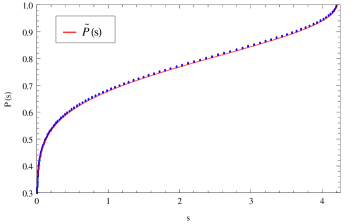
Figure 2: Circles represent cumulative spacing distribution $P(s)$, while continuous line is its analytic approximation $\tilde{P}(s)$ drawn for $N=20$ and $m_{1}=3,~{}m_{2}=1$.

7 Conclusions

In this paper we construct the PSRO (2.24) which, along with the spin exchange operator (2.25), yields a class of representations for the $BC_{N}$ type of Weyl algebra in the internal space associated with $N$ number of particles or lattice sites. This PSRO allows us to find out novel exactly solvable variants (3.1) of the $BC_{N}$ type of spin Calogero model. Taking the strong coupling limit of these spin Calogero models and also using the freezing trick, we obtain the $BC_{N}$ type of PF spin chains with PSRO (3.9). In one limit, these spin chains reproduce the $BC_{N}$ type of PF models studied by Enciso et. al. [38]. In another limit, these spin chains yield new SA type generalization (1.2) of the PF spin chain.

Subsequently, we construct some (nonorthonormal) basis vectors for the Hilbert spaces of the $BC_{N}$ type of spin Calogero models with PSRO by using the projector (3.26) and derive the exact spectra of the these models by taking advantage of the fact that their Hamiltonians can be represented in triangular form while acting on the above mentioned basis vectors. Then we apply the freezing trick to compute the partition functions (3.40) for the $BC_{N}$ type of PF spin chains with PSRO. Furthermore, we derive a remarkable relation (4.6) between the partition function of the $BC_{N}$ type of PF spin chain with PSRO and that of the $A_{N-1}$ type of PF spin chain. This relation turns out to be very efficient in studying spectral properties like level density and distribution of spacings for consecutive levels in the case of $BC_{N}$ type of PF spin chains with PSRO. We find that, similar to the case of many other quantum integrable spin chains with long-range interaction, the level density of these spin chains follows the Gaussian distribution and the cumulative distribution of spacing for consecutive levels follows a ‘square root of a logarithm’ law.

Taking a particular limit of the relation (4.6) we obtain Eq. (4.9), which implies that the spectrum of the SA type generalization of the PF spin chain (1.2) with arbitrary value of the parameter $\beta$ would coincide with that of the scaled Hamiltonian (4.4) for $A_{N-1}$ type of PF spin chain. This result is rather surprising, since the forms of the two above mentioned Hamiltonians apparently differ from each other. For the purpose of making some connection between these two apparently different types of Hamiltonians, we conjecture the asymptotic relation (4.11) between the (ordered) zero points of the Hermite polynomial and the generalized Laguerre polynomial. If this conjecture is correct, then the scaled Hamiltonian (4.4) of the $A_{N-1}$ type of PF spin chain can be seen as a particular limit of the Hamiltonian (1.2) corresponding to the SA type generalization of the PF spin chain. However, we have only verified the conjecture (4.11) analytically for the case of $N=2$ and numerically for $N=3$ and $N=4$. Therefore, finding out an analytical proof of the conjecture (4.11) might be an interesting problem to study from the viewpoint of orthogonal polynomials.

Finally it should be noted that, apart from the context of the $BC_{N}$ type of spin Calogero model and PF spin chain, the $BC_{N}$ type of Weyl algebra plays a very important role in context of the $BC_{N}$ type of spin Sutherland model, related HS spin chain and also for the cases of supersymmetric generalizations of these models [37, 56]. Therefore, one can use the PSRO (2.24) to construct novel exactly solvable variants of the $BC_{N}$ type of spin Sutherland model and HS spin chain [57]. Furthermore, it is also possible to construct supersymmetric generalization of the PSRO (2.24) and apply such operator to find out exactly solvable variants of the supersymmetric spin Calogero model and PF spin chain associated with the $BC_{N}$ root system [58].

Acknowledgements

We thank Artemio González-López and Federico Finkel for fruitful discussions.

References

• Calogero [1971] F. Calogero, J. Math. Phys. 12 (1971) 419–436.
• Sutherland [1971] B. Sutherland, Phys. Rev. A 4 (1971) 2019–2021.
• Sutherland [1972] B. Sutherland, Phys. Rev. A 5 (1972) 1372–1376.
• Olshanetsky and Perelomov [1983] M. A. Olshanetsky, A. M. Perelomov, Phys. Rep. 94 (1983) 313–404.
• Haldane [1988] F. D. M. Haldane, Phys. Rev. Lett. 60 (1988) 635–638.
• Shastry [1988] B. S. Shastry, Phys. Rev. Lett. 60 (1988) 639–642.
• Polychronakos [1993] A. P. Polychronakos, Phys. Rev. Lett. 70 (1993) 2329–2331.
• Polychronakos [1994] A. P. Polychronakos, Nucl. Phys. B 419 (1994) 553–566.
• Frahm [1993] H. Frahm, J. Phys. A: Math. Gen. 26 (1993) L473–L479.
• Finkel and González-López [2005] F. Finkel, A. González-López, Phys. Rev. B 72 (2005) 174411(6).
• Basu-Mallick et al. [1999] B. Basu-Mallick, H. Ujino, M. Wadati, J. Phys. Soc. Jpn. 68 (1999) 3219–3226.
• Basu-Mallick and Bondyopadhaya [2006] B. Basu-Mallick, N. Bondyopadhaya, Nucl. Phys. B 757 (2006) 280–302.
• Ha [1996] Z. N. C. Ha, Quantum Many-body Systems in one Dimension, volume 12 of Advances in Statistical Mechanics, World Scientific, Singapore, 1996.
• Murthy and Shankar [1994] M. V. N. Murthy, R. Shankar, Phys. Rev. Lett. 73 (1994) 3331–3334.
• Polychronakos [2006] A. P. Polychronakos, J. Phys. A: Math. Gen. 39 (2006) 12793–12845.
• Beenakker and Rajaei [1994] C. W. J. Beenakker, B. Rajaei, Phys. Rev. B 49 (1994) 7499–7510.
• Caselle [1995] M. Caselle, Phys. Rev. Lett. 74 (1995) 2776–2779.
• Beisert et al. [2003] N. Beisert, C. Kristjansen, M. Staudacher, Nucl. Phys. B 664 (2003) 131–184.
• Bargheer et al. [2009] T. Bargheer, N. Beisert, F. Loebbert, J. Phys. A: Math. Theor. 42 (2009) 285205(58).
• Beisert et al. [2012] N. Beisert et al., Lett. Math. Phys. 99 (2012) 3–32.
• Taniguchi et al. [1995] N. Taniguchi, B. S. Shastry, B. L. Altshuler, Phys. Rev. Lett. 75 (1995) 3724–3727.
• Forrester [1994] P. J. Forrester, Nucl. Phys. B 416 (1994) 377–385.
• Ujino and Wadati [1997] H. Ujino, M. Wadati, J. Phys. Soc. Jpn. 66 (1997) 345–350.
• Baker and Forrester [1997] T. H. Baker, P. J. Forrester, Nucl. Phys. B 492 (1997) 682–716.
• Bernard et al. [1993] D. Bernard, M. Gaudin, F. D. M. Haldane, V. Pasquier, J. Phys. A: Math. Gen. 26 (1993) 5219–5236.
• Hikami [1995] K. Hikami, Nucl. Phys. B 441 (1995) 530–548.
• Basu-Mallick [1999] B. Basu-Mallick, Nucl. Phys. B 540 (1999) 679–704.
• Hikami and Basu-Mallick [2000] K. Hikami, B. Basu-Mallick, Nucl. Phys. B 566 (2000) 511–528.
• Basu-Mallick et al. [2007] B. Basu-Mallick, N. Bondyopadhaya, K. Hikami, D. Sen, Nucl. Phys. B 782 (2007) 276–295.
• Basu-Mallick et al. [2008] B. Basu-Mallick, N. Bondyopadhaya, D. Sen, Nucl. Phys. B 795 (2008) 596–622.
• Ha and Haldane [1992] Z. N. C. Ha, F. D. M. Haldane, Phys. Rev. B 46 (1992) 9359–9368.
• Hikami and Wadati [1993] K. Hikami, M. Wadati, J. Phys. Soc. Jpn. 62 (1993) 469–472.
• Minahan and Polychronakos [1993] J. A. Minahan, A. P. Polychronakos, Phys. Lett. B 302 (1993) 265–270.
• Sutherland and Shastry [1993] B. Sutherland, B. S. Shastry, Phys. Rev. Lett. 71 (1993) 5–8.
• Bernard et al. [1995] D. Bernard, V. Pasquier, D. Serban, Europhys. Lett. 30 (1995) 301–306.
• Simons and Altshuler [1994] B. D. Simons, B. L. Altshuler, Phys. Rev. B 50 (1994) 1102–1105.
• Enciso et al. [2005] A. Enciso, F. Finkel, A. González-López, M. A. Rodríguez, Nucl. Phys. B 707 (2005) 553–576.
• Barba et al. [2008] J. C. Barba, F. Finkel, A. González-López, M. A. Rodríguez, Phys. Rev. B 77 (2008) 214422(10).
• Finkel et al. [2003] F. Finkel, D. Gómez-Ullate, A. González-López, M. A. Rodríguez, R. Zhdanov, Commun. Math. Phys. 233 (2003) 191–209.
• Caudrelier and Crampé [2004] V. Caudrelier, N. Crampé, J. Phys. A: Math. Gen. 37 (2004) 6285–6298.
• Yamamoto and Tsuchiya [1996] T. Yamamoto, O. Tsuchiya, J. Phys. A: Math. Gen. 29 (1996) 3977–3984.
• Finkel et al. [2001] F. Finkel, D. Gómez-Ullate, A. González-López, M. A. Rodríguez, R. Zhdanov, Commun. Math. Phys. 221 (2001) 477–497.
• Corrigan and Sasaki [2002] E. Corrigan, R. Sasaki, J. Phys. A: Math. Gen. 35 (2002) 7017–7061.
• Cigler [1979] J. Cigler, Monatsh. Math. 88 (1979) 87–105.
• Barba et al. [2008] J. C. Barba, F. Finkel, A. González-López, M. A. Rodríguez, Europhys. Lett. 83 (2008) 27005(6).
• Ahmed [1978] S. Ahmed, Lett. Nuovo Cimento 22 (1978) 371–375.
• Ahmed and Muldoon [1983] S. Ahmed, M. E. Muldoon, SIAM J. Math. Anal. 14 (1983) 372–382.
• Enciso et al. [2010] A. Enciso, F. Finkel, A. González-López, Phys. Rev. E 82 (2010) 051117.
• Banerjee and Basu-Mallick [2012] P. Banerjee, B. Basu-Mallick, J. Math. Phys. 53 (2012) 083301.
• Poilblanc et al. [1993] D. Poilblanc, T. Ziman, J. Bellissard, F. Mila, J. Montambaux, Europhys. Lett. 22 (1993) 537–542.
• d’Auriac et al. [2002] J.-C. A. d’Auriac, J.-M. Maillard, C. M. Viallet, J. Phys. A: Math. Gen. 35 (2002) 4801–4822.
• Basu-Mallick et al. [2010] B. Basu-Mallick, N. Bondyopadhaya, K. Hikami, SIGMA 6 (2010) 091–13.
• Haake [2001] F. Haake, Quantum Signatures of Chaos, Springer-Verlag, Berlin, second edition, 2001.
• Berry and Tabor [1977] M. V. Berry, M. Tabor, Proc. R. Soc. London Ser. A 356 (1977) 375–394.
• Basu-Mallick and Bondyopadhaya [2009] B. Basu-Mallick, N. Bondyopadhaya, Phys. Lett. A 373 (2009) 2831–2836.
• Barba et al. [2009] J. C. Barba, F. Finkel, A. González-López, M. A. Rodríguez, Nucl. Phys. B 806 (2009) 684–714.
• Basu-Mallick et al. [2014] B. Basu-Mallick, A. González-López, F. Finkel, Haldane-Shastry models of $BC_{N}$ type with polarized spin reversal operators (under preparation), 2014.
• Banerjee et al. [2014] P. Banerjee, B. Basu-Mallick, N. Bondyopadhaya, Supersymmetric extension of $BC_{N}$ type Polychronakos spin chains with polarized spin reversal operators (under preparation), 2014.