Modelling galaxy spectra at redshifts 0.2z 2.3
by the [OII]/H and [OIII]/H line ratios
We present the detailed modelling of line spectra emitted from galaxies at redshifts 0.2 z 2.3. The spectra account only for a few oxygen to H line ratios. The results show that [OII]3727+3729/H and [OIII]5007+4959/H are not sufficient to constrain the models. The data at least of an auroral line, e.g. [OIII]4363, should be known. We have found by modelling the spectra observed from ultrastrong emission line galaxy and faint galaxy samples, O/H relative abundances ranging between 1.810-4 and 6.610-4.
Key Words.:
radiation mechanisms: general — shock waves — ISM: O/H abundances — galaxies: starburst — galaxies: high redshift1 Introduction
Observations of line spectra emitted from galaxies at relatively high redshifts are now available (see Contini 2013b, hereafter Paper I, and references therein). Metallicities, in terms of the relative abundance of the heavy elements to H, have been calculated by a detailed modelling of the line ratios, providing some information about galaxy evolution, star formation rates, luminosities etc.
The spectra are relatively poor in number of lines at high z because only the strongest ones are observable. The modelling procedure, therefore, becomes problematic regarding model degeneracy.
Line ratios corresponding to different elements in a spectrum depend on the physical parameters and on the relative abundances of the elements. The O/H ratio shows generally the highest relative abundance compared with that of the other heavy elements whose lines are observed in the UV-optical -IR frequency range. Different solar O/H are reported by Asplund et al (2009), Allen (1976) and Anders & Grevesse (1989), namely, O/H=4.9 10-4, 6.6 10-4 and 8.5 10-4, respectively. Table 1 shows that Allen (1976) relative abundance values range between the two more recent results. Therefore, we will refer to Allen (1976). Yet, the relative abundances are calculated consistently for each spectrum. So the values which appear in Table 1 are important only as references for discussions.
| element | Allen | Anders & Grevesse | Asplund et al. |
|---|---|---|---|
| (1976) | (1989) | (2009) | |
| H | 12 | 12 | 12 |
| C | 8.52 | 8.56 | 8.43 |
| N | 7.96 | 8.05 | 7.83 |
| O | 8.82 | 8.93 | 8.69 |
| Ne | 8. | 8.09 | 7.93 |
| Mg | 7.4 | 7.58 | 7.6 |
| Si | 7.52 | 7.55 | 7.51 |
| S | 7.2 | 7.21 | 7.12 |
| Cl | 5.6 | 5.5 | 5.5 |
| Ar | 6.52 | 6.56 | 6.4 |
| Fe | 7.5 | 7.67 | 7.5 |
Line ratios from the same element in different ionization stages e.g. [OIII]5007+/[OII]3727+ (the + indicates that the 5007,4959 and 3727,3729 doublets are summed up), constrain the physical parameters such as the photoionization flux reaching the gas, the temperature of the line emitting gas, etc . The oxygen line ratios to H constrain the O/H relative abundance. So the ”direct” or method (Seaton 1975, Pagel et al. 1992, etc) is used to obtain O/H from the observed oxygen to H line ratios. By this method, the ranges of the gas physical conditions are chosen among those most suitable to the observed line ratios, e.g. the temperature is calculated from [OIII]5007+/[OIII] 4363, the temperature and the density ranges are constrained by [OII]3727+/H considering, in particular, that the critical density for collisional deexcitation of [OII] is 3000 . The density is constrained also by [SII] 6717/6731 line ratio, when observed.
In Paper I we have modelled the spectra of galaxies at redshifts between 0.001 and 3.4, on the basis of at least hydrogen, oxygen and nitrogen lines. We have adopted a composed model which accounts for the photoionization and for shocks.
In the present paper we deal with spectra showing a few oxygen line ratios to H , i.e. the [OIII] 5007+4959/H , [OIII]4363/H and [OII]3727+/H observation data reported by Kakazu et al (2007) for a sample of ultrastrong emission line galaxies at z1 and the [OIII] 5007+4959/H and [OII]3727+/H observation data reported by Xia et al. (2012) for a sample of faint galaxies at 0.6 z 2.4. Moreover, we have added a subsample of the stacking spectra of emission line galaxies at 1.3 z2.3 reported by Henry et al (2013). The stacking method is justified by the increasing number of data observed in the different galaxy samples.
Our aim is to discuss modelling degeneracy. We would like to find out the smallest set of oxygen line ratios to H suitable to constrain the O/H relative abundance. Moreover, we will compare the O/H results calculated by detailed modelling with those obtained by the other methods, e.g. the direct method and the metallicity calibrators (Perez-Montero & Diaz 2005 and references therein).
We will model the spectra, even those showing a few lines, by the method adopted for the spectra rich in number of lines (Paper I and references therein). Namely, the gas is ionized and heated by the black body radiation flux from the stars in the case of a starburst (SB) galaxy or by a power-law radiation flux from the active nucleus in active galactic nuclei (AGN).
It was found that galaxies at a relatively high z are the product of merging, therefore a shock dominated regime is assumed leading to compression and heating of the emitting gas downstream of the shock front. Collisional ionization and heating prevail on the radiation processes at relatively high shock velocities.
When the observed line spectrum of a galaxy contains a few hydrogen lines, oxygen lines from no more than two ionization stages, while the lines from the other elements are missing, the results of the calculation process can confront degeneracy. This refers at least to the abundances of the elements that are relatively strong coolants, whose lines are not seen. Carbon lines are not available in the optical range. Neon is hardly included into dust grains and molecules due to its atomic structure, therefore neon could be useful to investigate the evolution of the heavy elements with z, but its lines are weak. Even if Ne/H N/H, we will consider nitrogen as the second important heavy element because the N lines (e.g. [NII] 6584, 6548) observed from luminous galaxies at redshifts as high as z3.5 (Paper I) are relatively strong.
We will check this issue by the detailed modelling of the Kakazu et al (2007) sample of ultrastrong line emission galaxies and the Xia et al. (2012) faint galaxy sample.
In this paper we will first model the spectra adopting a solar N/H and discuss degeneracy by reducing the N/H relative abundance. In fact, the results obtained in Paper I dealing with spectra rich enough in number of lines, show that N/H splits from 10-4 to 10-5 at redshifts in the 0.2 z 1 range.
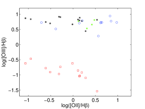
The observed spectra are relatively poor because many significant lines are missing (e.g. [NeIII], HeII, [OI], [NII] and [SII] etc) . Moreover, the trend of [OIII]5007+/H versus [OII]3727+/H (Fig. 1) indicates that the distribution of the data follows the ionization parameter rather than the O/H relative abundance, with some scattering due to the different physical conditions in the different objects.
To constrain the models by a first choice of the physical parameters, we have used the grids (Contini & Viegas 2001a,b) calculated previously by the SUMA code for SBs and AGNs. Then, we have refined the models in order to reproduce the observed line ratios.
In Sect. 2 the modelling method is presented. In Sect. 3 the Kakazu et al. (2007) sample is modelled. In Sect. 4 we deal with the Xia et al. (2012) spectra. The results of Henry et al (2013) sample galaxies appear in Sect. 5. Discussion and concluding remarks follow in Sect. 6.

2 Modelling method
2.1 Input parameters
The code suma111http://wise-obs.tau.ac.il/marcel/suma/index.htm is adopted for the calculation of the spectra, because it simulates the physical conditions in an emitting gaseous cloud under the coupled effect of photoionization from an external radiation source and shocks. The line and continuum emissions from the gas are calculated consistently with dust-reprocessed radiation in a plane-parallel geometry (see Contini et al 2009 and references therein for a detailed description of the code).
The input parameters are : the shock velocity , the preshock density , the preshock magnetic filed , which depend on the shock.
The ionization parameter and the effective star temperature define the ionization flux for starburst galaxies. A pure black body radiation referring to is a poor approximation for a starburst, even adopting a dominant spectral type (cf. Rigby & Rieke 2004). However, the line ratios which are used to indicate also depend on metallicity, electron temperature, density, ionization parameter, the morphology of the ionized clouds and, in particular, they depend on the hydrodynamical field.
The input parameter that represents the radiation field in AGNs is the power-law flux from the active nucleus in number of photons cm-2 s-1 eV-1 at the Lyman limit. The spectral indices are =-1.5 and =-0.7.
A magnetic field of 10-4 gauss is adopted for all the models. Moreover the relative abundances of the elements (He, C, N, O, Ne, Mg, Si, S, A, Cl, Fe) to H and the geometrical thickness of the emitting clouds are important factors.
The dust-to-gas () ratio is also an input parameter. It regards in particular the infrared frequency range of the continuum spectral energy distribution (SED), affecting the dust reprocessed radiation peak. The higher the intensity peak relative to the gas bremsstrahlung, the higher the ratio is. Moreover, a high can reduce a non radiative to a radiative shock (Contini 2004a) by mutual heating and cooling of dust and gas. We have no data for the continuum SED in the frequency range characteristic of the dust reradiation peak for the galaxies in the present samples, therefore we cannot determine exactly the ratio. We adopted an average =0.003 which is valid for starbursts.
The ranges of the input parameters are chosen with the following criteria. When the FWHM of the line profiles are not reported by the observations, we obtain a first hint about the shock velocity from the grids of models calculated for AGN and SB (Contini & Viegas 2001a,b). affects in particular the [OII] 3727+3729/H line ratio. The density of the emitting gas could be deduced from the [SII]6717/6731 line ratios, when these lines are observed, because the [OII] doublet 3727,3729 lines in galaxy spectra are generally blended. The temperature of the starburst and the ionization parameter are determined directly from the fit of the line ratios, in particular [OIII]5007+4959/H and HeII/H .
The geometrical thickness of the clouds () is a crucial parameter that can hardly be deduced from the observations. Indeed, in the turbulent regime created by shocks, Rayleigh-Taylor and Kelvin-Helmholtz instabilities cause fragmentation of matter that leads to clouds with very different geometrical thickness coexisting in the same region.
2.2 Modelling steps
The main differences between the direct method and the modelling by the code are described in the following.
The direct method derives from the oxygen lines (e.g. [OIII]5007 and [OII]3727) the physical conditions of the gas, in order to calculate the element abundances. The temperature of the emitting gas is obtained by considering the auroral line [OIII]4363. In brief, the direct method refers to the temperatures and densities most appropriated to the observed line ratios.
By the code, the temperatures and the densities and the fractional abundances of the ions that lead to specific line ratios, are all consistently calculated adopting a source of photoionization and heating of the gas (e.g. an SB or an AGN and/or shocks) throughout a cloud with certain characteristics. Moreover, the line intensities are all contemporarily calculated integrating throughout the cloud, which is cut in a certain number of slabs up to a maximum of 300.
The contribution of gas slabs in different conditions is the main cause of the different relative abundances calculated by the direct method and by modelling. In fact, the line intensity increment corresponding to a certain ion calculated by the model, can be low in regions where the gas conditions are less adapted. The contribution of these regions to the integration process leads to a weaker line. Therefore, to reproduce the observed line ratio to H , a relative abundance higher than that used by the direct method is adopted.
Very schematically, by modelling :
1) we adopt an initial input parameter set on the basis of the galaxy observations;
2) calculate the density in the slab of gas downstream from the compression equation;
3) calculate the fractional abundances of the ions from each level for each element;
4) calculate line emission, free-free and free - bound emission;
5) recalculate the temperature of the gas in the slab by thermal balancing or the enthalpy equation;
6) calculate the optical depth of the slab and the primary and secondary fluxes;
7) adopt the parameters found in slab i as initial conditions for slab i+1.
8) Integrating on the contribution of the line intensities calculated in each slab, we obtain the absolute fluxes of each of the lines, calculated at the nebula (the same for bremsstrahlung).
9) We then calculate the line ratios to a certain line (in the present case H )
10) and compare them with the observed line ratios.
The observed data have errors, both random and systematic. Models are generally allowed to reproduce the data within a factor of 2. This leads to input parameter ranges of a few per cent. The uncertainty in the calculation results (within 10 %) derives from the use of many atomic parameters, such as recombination coefficients, collision strengths etc., which are continuously updated. Moreover, the precision of the integrations depends on the computer efficiency.
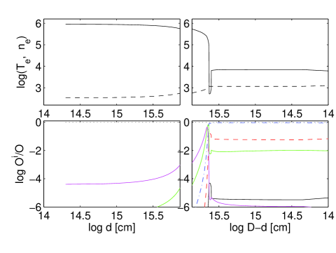
Notice that the profiles of the ions follow the profiles of the physical parameters throughout a cloud (as can be seen in Figs. 2 and 3) , therefore each line ratio corresponds to a series of temperatures and densities of the emitting gas.
If the calculated spectrum does not fit the data, the calculations are restarted changing the input parameters. We generally make a grid of models which is completed when the modelling results reproduce satisfactorily the data. The role of the grid consists in showing which of the parameters are critical to the various line ratios. By changing the input parameters (cross-checking all the line ratios for each model) the set which reproduces the data can be selected.
The grid is calculated by the following steps :
First we study in details all the characteristics of the galaxy in order to provide a first guess of the input parameters. Then, we consider the highest line ratio (generally, [OIII]5007/H ) and we test which of the input parameters is the key to fit the [OIII]/H line ratio. We try to reproduce [OII]/H and [NII/H changing the physical parameters. By cross-checking the [OIII]/H ratio, all the process will be restarted many times until a fine tune of all the lines is achieved. If some line ratios are not fitted, whichever the set of the physical parameters, we change the relative abundances until all the data are reproduced within about 20% for the strong lines and 50% for the weak lines.
2.3 Relevant issues
From the modelling point of view, once the physical conditions of the emitting gas and the photoionizing flux type and intensity are determined by the appropriated line ratios, the geometrical thickness of the cloud is deduced from the ratio between relatively high and low ionization level lines. In fact, larger clouds will contain a larger volume of gas at a relatively low temperature, leading to stronger low ionization level lines. The choice of , within the range of the observational evidence, is then constrained by the best fit of different line ratios. The clouds are matter-bound or radiation-bound depending on the geometrical thickness as well as on , and .
The coupled effect of radiation and shock determines the electron temperature and electron density of the gas and the fractional abundances of the ions corresponding to the line spectra. , and depend on the mutual heating (by radiation and by collision) and cooling (by recombination) throughout the gaseous clouds. Therefore, the emitting gas, even if it is described by a single model referring to one set of initial physical parameters and element abundances, does not show uniform conditions. For instance, the temperatures of the emitting gas range between T 1.45 105 ( / [100 ])2 in the downstream region close to the shock front and Tmin 103 K corresponding to the low ionization level and neutral gas. The gas cools down and recombines. The cooling rate depends on free-free, free-bound radiation and line emission. The line emission term accounts for the gas composition, i.e. for the abundances of all the elements composing the gas, even for those elements whose lines are not observed. The higher the element abundances, the higher the energy loss rates of the gas by line emission. The gradient of the temperature drop downstream close or far from the shock front depends on , and on the abundances of the elements. So a different O/H leads to different line ratios in general and to different oxygen to H line ratios, in particular.
When the gas clouds are ejected from the starburst, the shock front corresponds to the external edge of the cloud and the photoionizing (primary) flux from the stars reaches the opposite edge. The line intensities are emitted from the region downstream of the shock front, from the internal region of the cloud and from the region facing the stars. These regions are bridged by the secondary diffuse radiation flux which is calculated as well as the primary flux by radiation transfer throughout the nebula. When the cloud is geometrical thin and the primary flux is strong, the cool region inside the nebula is very reduced (see Figs. 2 and 3).
When both [OIII]/H and [OII]/H line ratios overpredict the data, we tend to reduce O/H. However, it is evident that this will yield different [OIII]/[OII] line ratios which must be readjusted by changing (or and in the SB case), , and/or . The cross-checking process sometimes ends with unpredictable results for O/H and the line ratios will be better reproduced by focusing on the physical parameters.
The calculation of even a single line flux needs all the physical and chemical parameters which appear for each model.
The absolute line fluxes referring to the ionization level i of element K are calculated by the term nK(i) which represents the density of the ion X(i). We consider that nK(i) = X(i)[K/H]nH, where X(i) is the fractional abundance of the ion i calculated by the ionization equations, [K/H] is the relative abundance of the element K to H and nH is the density of H (by number ). So the abundances of the elements are given relative to H as input parameters. In models including the shock, compression (nH/) downstream is calculated by the Rankine-Hugoniot equations for the conservation of mass, momentum and energy throughout the shock front.
In this paper, we discuss the modelling of a galaxy on the basis of the [OIII] 5007+/H , [OII] 3727+/H line ratios and eventually on [OIII] 4363/H . Actually, the [OIII] 4363 line (generally weak and blended with H) is not the most suitable choice to constrain the models, but if we aim to have some information for objects at high redshift, there is no alternative.
3 The line ratios from the Kakazu et al. (2007) galaxy sample
| ID | z | [OIII]5007+ | [OIII]4363 | [OII]3727+ | O/H | H abs | ||||||
|---|---|---|---|---|---|---|---|---|---|---|---|---|
| 104K | - | 10-4 | cm | |||||||||
| NB816 | ||||||||||||
| 40 | 0.629 | 7.690.3 | 0.0940.034 | 1.410.062 | - | - | - | - | - | - | - | |
| calc | - | 7.3 | 0.1 | 1.3 | 200 | 200 | 5. | 0.05 | 6.6 | 5e15 | 0.005 | |
| 76 | 0.6319 | 6.550.16 | 0.029 | 3.440.08 | - | - | - | - | - | - | - | |
| calc | - | 7.6 | 0.022 | 3.5 | 200 | 70 | 2.2 | 7.6 | 6.6 | 1.5e17 | 0.0056 | |
| 118 | 0.6439 | 6.870.43 | 0.340.13 | 0.1130.026 | - | - | - | - | - | - | - | |
| calc | - | 7. | 0.26 | 0.16 | 250 | 70 | 4.4 | 1. | 6.0 | 1.5e16 | 2.9e-4 | |
| 195 | 0.628 | 4.650.03 | 0.240.11 | 0.97 0.097 | - | - | - | - | - | - | - | |
| calc | - | 4.61 | 0.15 | 0.7 | 230 | 110 | 2.3 | 6.5 | 3. | 4.e16 | 0.0056 | |
| 252 | 0.64 | 6.250.13 | 0.090.04 | 1.390.037 | - | - | - | - | - | - | - | |
| calc | - | 6.1 | 0.094 | 1.1 | 200 | 200 | 5 | 0.05 | 6.5 | 5.e15 | 0.0064 | |
| NB912 | ||||||||||||
| 3 | 0.82 | 7.390.18 | 0.240.08 | 0.0860.025 | - | - | - | - | - | - | - | - |
| calc | - | 7.5 | 0.23 | 0.11 | 250 | 70 | 4.5 | 1.3 | 6.0 | 1.5e16 | 2.8e-4 | |
| 6 | 0.83 | 8.040.49 | 0.1840.11 | 0.520.086 | - | - | - | - | - | - | - | |
| calc | - | 9.5 | 0.07 | 0.54 | 200 | 150 | 3. | 1.7 | 4.2 | 6.e15 | 0.0013 | |
| 9 | 0.833 | 5.970.22 | 0.12 | 1.570.069 | - | - | - | - | - | - | - | |
| calc | - | 6. | 0.04 | 1.6 | 150 | 80 | 2.5 | 2. | 2. | 1.e17 | 0.0029 | |
| 10 | 0.829 | 6.690.17 | 0.140.044 | 1.290.053 | - | - | - | - | - | - | - | |
| calc | - | 7.0 | 0.147 | 1.3 | 200 | 200 | 4. | 0.12 | 6.6 | 4.e15 | 0.0034 | |
| 20 | 0.820 | 5.540.24 | 0.1680.055 | 0.2450.025 | - | - | - | - | - | - | - | |
| calc | - | 5.4 | 0.22 | 0.2 | 250 | 70 | 3.9 | 1. | 6.0 | 1.5e16 | 3.3e-4 | |
| 239 | 0.8273 | 2.780.17 | 0.08 | 1.910.1 | - | - | - | - | - | - | - | |
| calc | - | 2.73 | 0.072 | 1.6 | 200 | 200 | 3.8 | 0.05 | 6.5 | 5.e15 | 0.0067 | |
| 270 | 0.8176 | 5. 0.23 | 0.1240.034 | 0.3070.027 | - | - | - | - | - | - | - | |
| calc | - | 5. | 0.11 | 0.2 | 250 | 80 | 3.8 | 0.8 | 6.5 | 1.5e16 | 0.0011 | |
| 60 1 | 0.393 | 8.260.46 | 0.1070.078 | 0.4840.087 | - | - | - | - | - | - | - | |
| calc | - | 8.29 | 0.107 | 0.68 | 200 | 200 | 5. | 0.1 | 6.6 | 5.e15 | 0.0058 |
1 H emitter
Narrowband observations by the 10m Keck II telescope of ultrastrong emission line galaxies were presented by Kakazu et al. The spectra refer to galaxies which show the [OIII] 5007+, [OIII] 4363, [OII] 3727+ and H at redshifts z 1 and Ly emitting galaxies at redshift z5. The final sample consists of 267 galaxies in the NB816 filter and 275 in the NB912 filter. The ultrastrong emission line (USEL) galaxy data were obtained from intermediate resolution (R 1000) spectroscopy for a subsample of 18 objects that were specifically selected for a metallicity study by Kakazu et al.
We refer to the spectra from the objects selected by Kakazu et al and presented in their tables 4 and 5. The observed (reddening corrected) line ratios to H =1 are reported in Table 2 in the rows showing the ID number of the galaxy. In the next rows the calculated line ratios are given. We have used the models referring to the starburst because the single galaxy luminosities are most probably due to the starbursts and the SFR is rather high at redshifts 0.6-0.8 corresponding to the observed spectra (Kakazu et al 2007). In our sample we neglect the galaxies where [OII] 3727+ /H are missing or are indicated as upper limits. In Table 2 the redshift is reported in column 2 and the line ratios appear in columns 3, 4 and 5.
The errors in the observational data include uncertainties in the extinction and the gaussian fit to the line profiles. The underlying stellar population affects the continuum SED. Then, the relative intensity of the different lines will be affected when subtracting the underlying continuum with different precision. This yields another source of uncertainty in the results.
The errors in the calculation results depend on the uncertainties of the various coefficients and cross sections and on the physical processes included in the models.
In Table 2 columns 6-12 the input parameters which yield the best fit to the data follow. In column 12 the absolute H flux in calculated at the nebula is presented. A large gap (by a factor of 1014) between the calculated and observed H ( 10-17 , Kakazu et al, fig. 7) can be noticed because H is observed at Earth but calculated at the cloud. The gap depends on the square ratio of the distance of the emitting cloud from the hot radiation source and the distance of the galaxy to Earth.
The results presented in Table 2 show that 1) the ionization parameter is relatively high in the NB816 galaxies with ID=76 and 195, indicating that these objects are relatively compact, namely, the emitting clouds are close to the radiation source and/or that the radiation flux reaches the emitting cloud undisturbed by dusty and gaseous clumps in the interstellar medium. For the NB912 galaxy sample at higher z (except ID 60 at z=0.393 in the bottom rows) the corresponding ionization parameters are lower.
2) The temperature of the stars in average is similar to that calculated for SB galaxies in the same z range (Paper I). The shock velocities are in the norm, and the preshock densities range between 70 and 200 . Relatively low , low and a high may suggest an old age for these galaxies.
3) The O/H relative abundances are solar in nearly all the objects with minima of half and 0.3 solar in NB912 ID= 195 and 9, respectively. They result from model calculations.
The O/H calculated by Kakazu et al by the direct method are lower than solar. In fact, the lack of data did not permit an accurate evaluation of the gas physical conditions. Let us try to obtain an acceptable fit to the observed line ratios adopting a model with a lower O/H. We focus on the galaxy ID 270 from the NB912 sample. The observed line ratios are [OIII]5007+/H =5.0, [OIII]4363/H =0.124 and [OII] 3727+/H =0.307 (Table 1, row 4 from bottom). Adopting O/H =1.8 10-4, =100 , =100 =0.4 and =1.5 1017 cm, we obtain [OIII[5007+/H =5.1 and [OII]3727+/H = 0.31, in good agreement with the data. However, [OIII]4363/H =0.03 is low compared with the observed value (0.124).
Modelling the [OIII]4363/H line ratios one should take into consideration that the [OIII]4363 line is generally blended with H. The O++/O fractional abundance is at maximum at temperatures 104 - 105 K. The theoretical H /H line ratios (Osterbrock 1989) corresponding to these temperatures are 0.45-0.46. So [OIII]4363/H constrains the O/H relative abundance (and the physical conditions) in the galaxies, only if [OIII]4363 is uncontaminated from blending and it is strong enough. In this work we have constrained the models presented in Table 2 by the [OIII]4363/H line ratios, considering that the data presented by Kakazu et al for [OIII] 4363 refer to this line only.
To better understand the line ratios emitted from the ID 270 galaxy we present in Figs. 2 and 3 the distribution of the electron temperature , the electron density and of the fractional abundance of the oxygen ions and of H+/H throughout a cloud moving outwards from the SB. The emitting cloud is divided into two halves represented by the left and right diagrams. The left diagrams show the region close to the shock front and the distance from the shock front on the X-axis scale is logarithmic. The right diagrams show the conditions downstream far from the shock front, close to the edge reached by the photoionization flux which is opposite to the shock front. The distance from the illuminated edge is given by a reverse logarithmic X-axis scale. In Fig. 2 the results refer to the model reported in Table 2, while in Fig. 3 the results refer to the model calculated by a relatively low O/H (1.8 10-4).
Fig. 2 shows that the high temperature of the gas downstream ( 105 K) depends on the shock velocity. The temperature is 104 K close to the cloud edge heated and ionized by the radiation flux from the star. The O2+ and the H+ ions dominate a large region of the clouds. The [OIII]4363/[OIII]5007 line ratio is higher in the model calculated by a higher because the temperature is high in a large zone of the cloud downstream.
4 The line ratios from the Xia et al (2012) galaxy sample
| ID | z | [O II]37271 | H 1 | [O III]50071 |
|---|---|---|---|---|
| 339 | 0.602 | 645.51162.65 | 468.4145.19 | 2373.9556.24 |
| 364 | 0.642 | 80.9015.93 | 50.357.24 | 308.619.59 |
| 246 | 0.696 | 4.504.50 | 22.905.22 2 | 21.916.92 |
| 454 | 0.847 | 166.5717.8 | 45.2213.921 | 86.3518.02 |
| 258 | 0.998 | 29.984.25 | 73.6335.74 | 241.9147.48 |
| 432 | 1.573 | 101.9723. | 24.2111.76 | 132.1115.56 |
| 563 | 1.673 | 93.9117.3 | 13.959.06 | 122.0411.86 |
| 103 | 1.682 | 43.5510.2 | 9.847.81 | 2.8310.33 |
| 195 | 1.745 | 87.8413.87 | 21.258.28 | 109.8710.91 |
| 242 | 2.070 | 94.7929.03 | 13.398.57 | 79.4611.19 |
| 578 | 2.315 | 116.5821.06 | 12.2910.42 | 65.9813.53 |
1 in 10-18
| ID | z | [OIII]5007+ | [OII]3727+ | O/H | H abs | H obs | |||||
|---|---|---|---|---|---|---|---|---|---|---|---|
| 104K | 10-4 | cm | 10-18 | ||||||||
| 339 | 0.602 | 5.07 | 1.38 | - | - | - | - | - | 468.41 45.19 | ||
| calc | - | 5.4 | 1.3 | 200 | 80 | 2.4 | 5.2 | 1.8 | 1.e17 | 5.1e-3 | - |
| 364 | 0.642 | 6.13 | 1.61 | - | - | - | - | - | - | - | 50.35 7.24 |
| calc | - | 6.0 | 1.61 | 150 | 80 | 2.5 | 2. | 2. | 1.e17 | 2.9e-3 | - |
| 246 | 0.696 | 5.32 | 0.196 | - | - | - | - | - | - | - | 22.905.22 |
| calc | - | 5.0 | 0.2 | 250 | 80 | 3. | 0.8 | 6.6 | 1.5e16 | 1.13e-3 | - |
| 454 | 0.847 | 1.91 | 3.68 | - | - | - | - | - | - | - | 45.2213.92 |
| calc | - | 2.1 | 3.2 | 250 | 180 | 1.4 | 0.003 | 6.6 | 5.e15 | 2.6e-3 | - |
| 258 | 0.998 | 3.28 | 0.41 | - | - | - | - | - | - | - | 73.6335.74∗ |
| calc | - | 3.66 | 0.44 | 280 | 100 | 3. | 0.9 | 5.6 | 1.2e16 | 1.5e-3 | - |
| 432 | 1.573 | 5.46 | 4.2 | - | - | - | - | - | - | - | 24.2111.76∗ |
| calc | - | 5.5 | 4.4 | 200 | 70 | 2.1 | 7. | 6.2 | 1.4e17 | 5.3e-3 | - |
| 563 | 1.673 | 8.75 | 6.73 | - | - | - | - | - | - | - | 13.959.06∗ |
| calc | - | 8.63 | 6.1 | 200 | 70 | 2.1 | 7. | 6.2 | 1.3e17 | 3.8e-3 | - |
| 103 | 1.682 | 5.37 | 4.43 | - | - | - | - | - | - | - | 9.847.81∗ |
| calc | - | 5.5 | 4.4 | 200 | 70 | 2.1 | 7. | 6.2 | 1.4e17 | 5.3e-3 | - |
| 195 | 1.745 | 5.17 | 4.13 | - | - | - | - | - | - | - | 21.258.28∗ |
| calc | - | 5.23 | 4.2 | 200 | 70 | 2.1 | 7. | 5. | 1.44e17 | 5.23e-3 | - |
| 242 | 2.070 | 5.93 | 7.08 | - | - | - | - | - | - | - | 13.398.57∗ |
| calc | - | 5.22 | 7.6 | 250 | 165 | 1.4 | 0.003 | 4.6 | 5.e15 | 7.6e-4 | - |
| 578 | 2.315 | 5.37 | 9.48 | - | - | - | - | - | - | - | 12.2910.42∗ |
| calc | - | 5.9 | 9.2 | 250 | 165 | 1.4 | 0.001 | 4.6 | 5.e15 | 6.7e-4 | - |
∗ The 3 upper limit of the H line is used for galaxies with S/N 3.
| ID | z | [OII]3727+ | [OIII]5007+ | H | H (abs) | O/H | ||||||
|---|---|---|---|---|---|---|---|---|---|---|---|---|
| - | - | - | - | units1 | 104 K | - | 1018 cm | 10-4 | ||||
| 1 | 1.82 | 1.32 | 5.891.23 | 3.6 | - | - | - | - | - | - | - | - |
| m1SB | - | 1.3 | 6. | 2.94 | 0.093 | 180 | 200 | - | 6 | 0.2 | 5 | 6.6 |
| m1AGN | - | 1.58 | 5.5 | 3.3 | 0.118 | 130 | 270 | 5 | - | - | 7 | 4. |
| 2 | 1.73 | 3. | 6.451.2 | 3.6 | - | - | - | - | - | - | - | - |
| m2SB | - | 3.1 | 6.3 | 2.93 | 0.045 | 240 | 200 | - | 7.6 | 0.04 | 9 | 6.6 |
| m2AGN | - | 2.9 | 6.5 | 3.3 | 0.065 | 130 | 220 | 2.3 | - | - | 7 | 6. |
| 3 | 1.77 | 2.64 | 4.571.15 | 3.6 | - | - | - | - | - | - | - | - |
| m3SB | - | 2.6 | 4.58 | 2.94 | 0.043 | 180 | 220 | - | 6.3 | 0.036 | 7 | 6.6 |
| m3AGN | - | 2.5 | 4.85 | 3.44 | 0.079 | 160 | 260 | 2.1 | - | - | 7 | 6.6 |
| 4 | 1.74 | 2.04 | 3.41.17 | 3.6 | - | - | - | - | - | - | - | - |
| m4SB | - | 2.1 | 3.4 | 2.94 | 0.051 | 180 | 240 | - | 5.6 | 0.04 | 5 | 6.6 |
| m4AGN | - | 2.04 | 3.37 | 3.5 | 0.106 | 130 | 260 | 2. | - | - | 9 | 6.0 |
1 1010 photons cm-2 s-1 eV-1 at the Lyman limit
Xia et al (2012) presented the spectra of faint galaxies at 0.6z2.4 observed by Advanced Camera for Surveys (ACS) on the Hubble Space Telescope (HST) and in the near-infrared using Wide-Field Camera 3. Xia et al data come from low resolution (R 100) grism spectroscopy in which even the H -[OIII] lines are heavily blended.
The line flux uncertainties are shown in Table 3. The modelling results of the [OII] 3727+/H and [OIII] 5007+/H line ratios are shown in Table 4. Table 4 array is similar to that of Table 2. In the last column of Table 4 the observed H fluxes are given.
The spectra presented by Xia et al show the minimum number of lines which can yield reliable results. In fact, we have run a grid of many models ( 30) for each spectrum before selecting the line ratios best fitting the data.
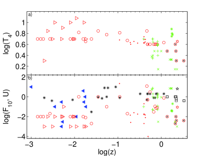
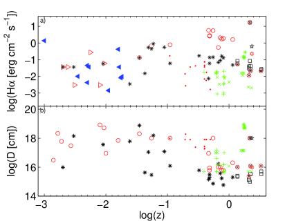
The results for the whole sample show rather low ( 3 104 K) and ranging throughout four orders. The shock velocities and the preshock densities are in the ranges calculated for the Kakazu et al sample (Fig. 4), lower than those for SB and AGN which are shown in Fig. 5. Actually in Fig. 5 we report the results presented in Paper I.
The O/H relative abundances are about solar at 0.696 z 1.745, 0.3 solar for galaxies at 0.602 and 0.642 and increase to 0.7 solar at z2.
We have chosen the spectrum observed from the galaxy ID 195 (Table 4, row 6 from bottom) to investigate degeneracy. The detailed modelling of the [OII]3727+/H and [OIII]5007+/H line ratios leads to O/H=5. 10-4. This corresponds to 12+log(O/H)=8.7, while Xia et al. obtained 8.38 (-0.27) adopting metallicity calibrators. We have tried to fit the oxygen line ratios by a lower O/H. We have found [OII]/H =4.54 and [OIII]/H =5.43 in very good agreement with the data (Table 4) adopting O/H = 1. 10-4 (12+log(O/H)=8.), =200 , =67 , =1.9 104, =6.8, =9.1016 cm. Indeed the modelling of the Xia et al spectra shows degeneracy. However, the model presented for ID 195 in Table 4 yields [OIII]4363/H = 0.017, while the model calculated with a low O/H shows [OIII]4363/H = 0.144. [OIII]4363/H ratios between 0.144 and 0.04 are reported by Kakazu et al. (Table 2). So they are both reasonable. In their paper, Xia et al. (2012) mention the weakness of the [OIII] 4363 line in the observed spectra. This information can be used to constrain the results, and it may indicate that the model calculated with a higher O/H (as that presented in Table 4) is more reliable.
5 Modelling the sample by Henry et al (2013)
Henry et al (2013) report mass-metallicity relation for log (M/M⊙) between 8 and 10 calculated by stacking spectra of 83 emission-line galaxies with redshifts 1.3 z 2.3. In their table 1 they present line ratio observations for four stacked galaxies at 1.74z 1.82, covering the ([OII]3727+3729 + [OIII]5007+4959)/H line ratios which are adapted to the metallicity diagnostic (Pagel et al.1979). In fact, Henry et al used the metallicity calibrator method. The sample is taken from Hubble Space Telescope Wide Field Camera 3 grism observations.
We expand our investigation on the O/H relative abundances calculated for galaxies on the basis of the [OII]/H and [OIII]/H lines including the Henry et al. (2013, table 1) observations. The spectra are not specific to single galaxies and must be considered as averages within small ranges. We refer to the reddening corrected data. Anyhow, the differences between the corrected and not corrected line ratios are within the observed errors.
In Table 5 we report the observed line ratios and compare them with model calculations results. The [OII] 3727+/H ratios were calculated from the Henry et al O32 ([OIII]5007+/[OII] 3727+) reported in their table 1. However, the errors of the [OII] 3727+/H line ratios cannot be calculated because the observed H fluxes are not given by Henry et al.
The data for each group of galaxies are followed by the calculation results in the next two rows, one referring to models calculated for the SB and the next for the AGN. In fact, Henry et al mention an eventual contribution to the SB of AGN spectra. Notice that the data refer to averaged spectra for a group of heterogeneous galaxies therefore the results of modelling should be considered only as approximations. The input parameters adopted by the models are presented in the last 7 columns of Table 5.
The results show that the O/H referring to the ID= 1 spectrum calculated by the AGN is 4.10-4. All the other galaxies show solar O/H = 6.0 - 6.6 10-4 (Allen et al 1976). Moreover, regarding the starburst, the star temperatures are 5.6 104 K. The radiation flux from the AGN components are similar to the lower limit of for AGN but higher than the low luminosity AGNs fluxes (e.g. Contini 2004b).
6 Discussion and concluding remarks
The spectra observed from the galaxies presented by Kakazu et al. and by Xia et al. surveys are employed to calculate the physical conditions of the emitting gas by a detailed modelling of ultrastrong emitting line galaxies and faint galaxies, respectively, at intermediate redshifts. Moreover, we have modelled the spectra presented by Henry et al which were obtained from the stacking of 85 luminous galaxies.
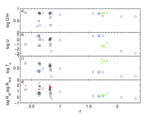
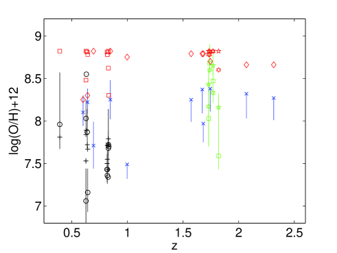
The results of the most significant parameters are shown in Fig. 4. The O/H ratios are shown in units of 10-4 and in units of 104 K. All the results presented in Tables 2, 4 and 5 are compared with those calculated for a much larger sample of galaxies in Fig. 5.


We have investigated whether the line ratio modelling results are constrained by the number and type of the observed lines, in terms of degeneracy. We have discussed, in particular, the Xia et al sample which do not show line ratios other than [OIII]5007+/H and [OII]3727+/H . The models are hardly constrained. To investigate the results found in Sect. 3 about the leading role of the [OIII] 4363 /H line ratio, we presented the following test. A first grid of models was run adopting O/H ratios as close to solar (Allen 1976) as those adopted to fit the sample of galaxies which appear in Paper I and in the Kakazu et al. sample. The O/H relative abundances were readjusted in order to best fit the data in tune with the other input parameters. The results appear in Table 4. Then, we recalculated the spectrum of the Xia et al ID 195 galaxy by O/H= 10-4 in agreement with the results obtained by the methods adopted by the other authors. The observed [OIII]5007+/H and [OII] 3727+/H ratios were reproduced by both high and low O/H models. To remove degeneracy we invoked the observed weakness of the [OIII] 4363 line. We conclude that spectra referring only to [OIII]5007+/H and [OII] 3727+/H cannot be modelled with precision without any further indication about e.g. the FWHM of the line profiles or the intensity of some other lines.
6.1 Results for different N/H
Let us now investigate the role of the abundances of elements different from oxygen. Actually, the Kakazu et al and Xia et al samples were chosen by our investigation because, due to the observing difficulties at those z, the lines corresponding to heavy elements, other than oxygen, were not reported. Those lines are generally weaker than the oxygen ones, and/or they cannot be easily deblended. Nevertheless, the gas is generally composed by the most prominent elements. We have used in the present models Allen (1976) solar abundances (He/H=0.1, C/H=3.3 10-4, N/H=9.1 10-5, O/H=6.6 10-4, Ne/H=1. 10-4, Mg/H=2.6 10-5, Si/H=3.3 10-5, S/H=1.6 10-5, Cl=4. 10-7, A/H=3.3 10-6, Fe/H=3.2 10-5).
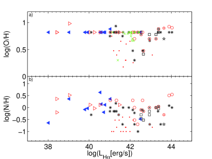
In Fig. 5 we have added to the modelling results calculated in Paper I the results calculated for the galaxy samples reported in the present work. The relatively large galaxy sample presented in Paper I, contains galaxies which were selected among those including at least the [NII]6548+6584 doublet, in order to minimize degeneracy. The O/H relative abundances presented in Tables 2, 4 and 5 follow the trend found for different types of galaxies (Fig. 5, left middle diagram).
Changing the abundance of one of the heavy elements relative to H, in particular for strong coolants e.g. O, N, etc, the results of the emitted line ratios would change. In fact, the relative abundance of each element affects not only the line intensity but also the cooling rate of the gas in the recombination zone.
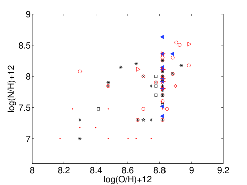
Let us investigate whether our models which adopt solar abundances for the elements corresponding to unobserved lines lead to trustful results. This is a critical test which could invalidate most of the results presented in this paper. In Paper I we have obtained by modelling the spectra reliable N/H and O/H for each galaxy. The N/H versus O/H relative abundances are shown in Fig. 6. Even with a large scattering, the data show that there is an increasing trend of N/H with O/H. So in order to investigate degeneracy which may result by changing the N/H input in a spectrum, we have run models with N/H lower than solar for galaxies which show a relatively low O/H.
We report in Table 6 the oxygen line ratios observed and calculated for two galaxies : ID 9 (NB912) from the Kakazu et al sample and ID 339 from the Xia et al sample. Both refer to a relatively low O/H (Tables 2 and 4). Table 6 shows that the N/H relative abundance does not affect the results as much as to imply a new set of the other input parameters. The observational error is 10% for most of the lines. On the other hand, changing the parameters such as , , and/or can lead to strong differences in the (oxygen) line ratios (see Contini & Viegas 2001a,b). Therefore, the results of the present work are safe concerning the physical conditions and the O/H relative abundance.
As confirmed by Fig. 6, different N/H can correspond to the solar O/H for many galaxies. The different N and O trends can be understood following Edmunds & Pagel (1978), namely, by the distinction between ’primary’ elements such as oxygen and the ’secondary’ ones. Nitrogen is a secondary element contaminated, however, by a non negligible primary component. Edmunds & Pagel suggest that although oxygen is instantaneously recycled by the supernova synthesis, nitrogen could be released by longer-lived stars and hence will appear in the ISM with a delay.
In other words, the scattering of the N/O abundances at a relatively constant O/H which appears at z 0.1 can be explained by a retarded release of N produced in low mass longer-lived stars compared with O produced in massive, short-lived stars (Mouhcine & Contini 2002).
| ID | z | [OIII]5007+ | [OIII]4363 | [OII]3727+ | O/H | N/H |
|---|---|---|---|---|---|---|
| 10-4 | 10-5 | |||||
| 9 1 | 0.833 | 5.97 | 0.12 | 1.57 | - | - |
| m1 | 6.0 | 0.037 | 1.62 | 2. | 10. | |
| m2 | 6.1 | 0.038 | 1.63 | 2. | 6. | |
| m3 | 6.16 | 0.039 | 1.65 | 2. | 2. | |
| m4 | 6.18 | 0.04 | 1.66 | 2. | 1. | |
| 339 2 | 0.602 | 5.07 | - | 1.38 | - | - |
| m11 | 5.42 | - | 1.30 | 1.8 | 10. | |
| m12 | 5.51 | - | 1.31 | 1.8 | 6. | |
| m13 | 5.54 | - | 1.33 | 1.8 | 2. | |
| m14 | 5.55 | - | 1.34 | 1.8 | 1. |
1 from the Kakazu et al. sample ; 2 from the Xia et al. sample
| ID | z | mod | KCH11 | KCH2 1 |
|---|---|---|---|---|
| NB816 | ||||
| 40 | 0.629 | 8.82 | 7.86 8.038.25 | 7.84 0.02 |
| 76 | 0.6319 | 8.82 | 8.55 | 7.890.01 |
| 118 | 0.6439 | 8.78 | 6.937.167.44 | 7.670.03 |
| 195 | 0.628 | 8.48 | 6.787.067.44 | 7.530.03 |
| 252 | 0.64 | 8.81 | 7.687.878.14 | 7.720.01 |
| NB912 | ||||
| 3 | 0.82 | 8.78 | 7.26 7.437.65 | 7.71 0.02 |
| 6 | 0.83 | 8.62 | 7.407.688.14 | 7.790.03 |
| 9 | 0.833 | 8.30 | 7.7 | 7.720.02 |
| 10 | 0.829 | 8.82 | 7.59 7.727.89 | 7.740.02 |
| 20 | 0.820 | 8.78 | 7.18 7.367.58 | 7.550.02 |
| 239 | 0.8273 | 8.81 | 7.34 | 7.430.02 |
| 270 | 0.8176 | 8.81 | 7.287.437.61 | 7.500.02 |
| 60 2 | 0.393 | 8.82 | 7.67 7.968.57 | 7.810.02 |
1 Kakazu et al (2007, tables 4 and 5). KCH1:data obtained by direct method, KCH2:data based on Yin et al (2007) method.
| ID | z | mod | Xia et al 1 | |
|---|---|---|---|---|
| 339 | 0.602 | 8.25 | 8.10 | |
| 364 | 0.642 | 8.30 | 8.22 | |
| 246 | 0.696 | 8.82 | 7.71 | |
| 454 | 0.847 | 8.82 | 8.25 | |
| 258 | 0.998 | 8.75 | 7.49 | |
| 432 | 1.573 | 8.79 | 8.25 | |
| 563 | 1.673 | 8.79 | 8.37 | |
| 103 | 1.682 | 8.79 | 7.97 | |
| 195 | 1.745 | 8.7 | 8.38 | |
| 242 | 2.070 | 8.66 | 8.32 | |
| 578 | 2.315 | 8.66 | 8.27 |
1 Xia et al (2012, table 2). Results obtained by R23 empirical calibrators.
| ID | z | modSB1 | modAGN2 | KK043 | Maiolino4 | FMR5 |
|---|---|---|---|---|---|---|
| 1 | 1.82 | 8.82 | 8.6 | 8.16 | 7.59 | - |
| 2 | 1.73 | 8.82 | 8.78 | 8.43 | 8.03 | 8.17 |
| 3 | 1.77 | 8.82 | 8.82 | 8.65 | 8.47 | 8.33 |
| 4 | 1.74 | 8.82 | 8.78 | 8.82 | 8.68 | 8.60 |
6.2 Comparison of the O/H results
Finally, we compare in Tables 7, 8 and 9 the results for O/H calculated by the present models and those determined by Kakazu et al., adopting the direct method and by Xia et al. and Henry et al. adopting empirical calibrators. Our results lead to O/H = 10-4 – 6.6 10-4.
Actually, the physical parameters adopted by Kakazu et al and Xia et al. to characterize the emitting gas are different from those determined by the best fit of the line ratios in the present paper, e.g. Kakazu et al fixed the electron density to =100 , because the line ratios, which depend directly on the density, were not observed. In our models ranges between 600 and 1000 due to compression (Fig. 2) and recombination downstream.
Moreover, Figs. 4 shows that SB star temperatures calculated for the Henry et al sample are higher than those calculated from the Xia et al sample and higher than those calculated for a large sample of galaxies in Fig. 5. The ionization parameters calculated for these stacked spectra are lower than those calculated for the Xia et al sample, but they are consistently located throughout the large sample presented in Fig. 5.
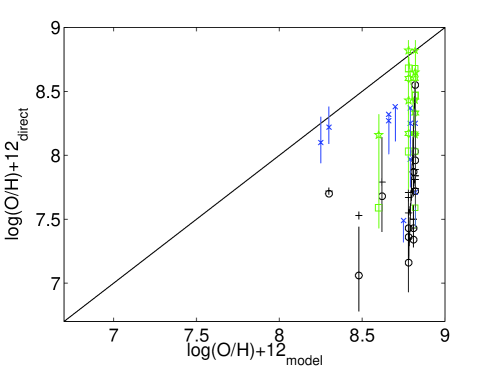
Figs. 7 and 8 show that a large gap appears between the O/H results obtained by the direct method (and that of Yin et al 2007) and those obtained by detailed calculations, however, the trend of O/H with z is roughly similar for our results and those of Xia et al for galaxies at z 1.
The large gap between our O/H results and those obtained by the direct method or by empirical calibrators has been explained in Sect. 2. Namely, the line intensities are calculated throughout a cloud integrating on regions showing different , and, consequently, different fractional abundances of the ions. Regions corresponding to relatively low contribute mostly to low ionization level lines, while a high contributes to relatively high ionization level lines. So the final [OIII] and [OII] line calculated intensities will be lower than those calculated adopting the optimum and . To reproduce the observed [OIII]/H line ratios a higher O/H is then needed by the model.
Concluding, the relative O/H abundances calculated by the direct method by Kakazu et al (2007) and empirical methods by Xia et al. (2012) and Henry et al. (2013) are lower limits because they adopted physical conditions in the emitting nebulae different from those consistently calculated by the detailed modelling.
The relatively high O/H ratios calculated in this paper reduce the low-metallicity character of galaxies at higher z. Moreover, Figs. 4, 5 and 8 confirm that the critical redshift for the scattering of metallicity started at z 1.
Finally, in this paper which deals with the modelling of relatively high redshift galaxies on the basis of [OIII]/H and [OII]/H observations, we claim that the [OIII]5007+/H and [OII]3727+/H line ratios alone are not sufficient to constrain the results.
Acknowledgements.
I am very grateful to the referee for many interesting remarks which improved the presentation of the paper.References
Allen, C.W. 1976 Astrophysical Quantities, London: Athlone (3rd edition)
Anders, E., Grevesse, N. 1989, Geochimica et Cosmochimica Acta, 53, 197
Asplund, M., Grevesse, N., Sauval, A.J., Scott, P. 2009, ARAA, 47, 481
Brand, K., et al. 2007, ApJ, 663, 204
Capetti, A., Robinson, A., Baldi, R. D., Buttiglione, S., Axon, D.J., Celotti, A., Chiaberge, M. 2013 arXiv1301.5757C
Contini, M. 2013a, MNRAS, 429, 242
Contini, M. 2013b, MNRAS submitted (Paper I), arXiv:1310.5447
Contini, M. 2009, MNRAS, 399, 1175
Contini, M. 2004a, A&A, 422, 591
Contini, M. 2004b, MNRAS, 354, 675
Contini, M. 1997, A&A, 323, 71
Contini, M., Viegas, S.M. 2001b, ApJS, 137, 75
Contini, M., Viegas, S.M. 2001a, ApJS, 132, 211
Diaz, A.I., Prieto, M. A., Wamsteker, W. 1988, A&A, 195, 53
Edmunds, M.G. & Pagel, B.E.J. 1978, MNRAS, 185, 77
Henry, A. et al 2013, arXiv:1309.4458
Kakazu, Y., Cowie, L.L., Hu, E.M. 2007, ApJ, 668, 853
Kobulnicky, H., Zaritsky, D. 1999, ApJ, 511, 118
Kobulnicky, H.A., Kewley, L.J. 2004, ApJ, 617,240 (KK04)
Krogager, J-K. et al. 2013, arXiv:1304.4231
Maiolino, R. et al. 2008 A&A, 488, 463
Mannucci, F., Salvaterra, R., Campisi, M. A. 2011, MNRAS, 414, 1263
Mouhcine, M. & Contini, T. 2002, A&A, 106, 114
Osterbrock, D.E. Astrophysics of Gaseous Nebulae and Active Galactic Nuclei. Mill Valley, CA: University Science Books; 1989.
Pagel, B.E.J., Simonson, E.A., Terlevich, R.J., Edmunds, M.G. 1992, MNRAS, 255, 325
Perez-Montero, E., Diaz, A.I. 2005, MNRAS, 361, 1063
Ramos Almeida, C., Rodríguez Espinosa, J.M., Acosta-Pulido, J.A. Alonso-Herrero, A., Pérez García, A.M, Rodríguez-Eugenio, N. 2013, MNRAS, 429, 3449
Rigby, J.R., Rieke, G.H. 2004 ApJ, 606, 237
Schirmer, M., Diaz, R., Holhjem, K., Levenson, N.A., Winge, C. 2013, ApJ, 763, 60
Seaton, M.J. 1975, MNRAS, 170, 475
Viegas, S.M., Contini, M., Contini, T. 1999, A&A, 347, 112
Winter, L.M., Lewis, K.T., Koss, M., Veilleux, S., Keeney, B., Muschotzky, R. 2010, ApJ, 710, 503
Xia, L. et al. 2012, AJ, 144, 28
Yin, S.Y., Liang, Y.C., Hammer, F., Brinchmann, J., Zhang, B., Deng, L.C., Flores, H. 2007, A&A, 462, 535 2010, ApJ, 710, 503