Direction Finding Algorithms with Joint Iterative Subspace Optimization

Abstract

In this paper, a reduced-rank scheme with joint iterative optimization is presented for direction of arrival estimation. A rank-reduction matrix and an auxiliary reduced-rank parameter vector are jointly optimized to calculate the output power with respect to each scanning angle. Subspace algorithms to estimate the rank-reduction matrix and the auxiliary vector are proposed. Simulations are performed to show that the proposed algorithms achieve an enhanced performance over existing algorithms in the studied scenarios.

I Introduction

In many array processing related fields such as radar, sonar, and wireless communications, the information of interest extracted from the received signals is the direction of arrival (DOA) of waves transmitted from radiating sources to the antenna array. The DOA estimation problem has received considerable attention in the last several decades [2]. Many estimation algorithms have been reported in the literature, e.g., [3], [4, Chapters 8 and 9], and the references therein. Among the most representative algorithms are Capon’s method [5], maximum-likelihood (ML) [6], and subspace-based schemes[7]-[25].

Capon’s method calculates the output power spectrum over the scanning angles and determines the DOA by locating the peaks in the spectrum. The implementation is relatively simple. The drawback of this method is that the resolution strongly depends on the number of available snapshots, the signal-to-noise ratio (SNR) and the array size. The ML type algorithms are robust for DOA estimation since they exhibit superior resolution in hostile scenarios with a low input SNR as long as the number of snapshots is small. Moreover, they work well when the sources are correlated. However, the implementation of the ML type methods is complicated and requires intensive computational cost, which limits their practical applications.

I-A Prior Work

Subspace-based algorithms, which exploit the structure of the received data to decompose the observation space into a signal subspace and a corresponding orthogonal noise subspace, play an important role for DOA estimation. According to the approach to compute the signal subspace, the subspace-based methods can be classified into eigen-decomposition, subspace tracking, and basis vectors based algorithms. Among the most popular and cost-effective eigen-decomposition algorithms are MUSIC [7] and ESPRIT [8] that require an eigen-decomposition. The MUSIC algorithm computes the output power spectrum by scanning the possible angles and selects the peaks to estimate the directions of the sources. The root MUSIC algorithm [4, pp. 1158-1163] and its low-complexity versions [9] have also been reported and shown to result in efficient DOA estimates. The ESPRIT algorithm employs a displacement invariance in some specific array structures and requires a lower complexity than MUSIC [4, pp. 1170-1194]. Iterative DOA estimation methods exploiting the removal of detected signals have been reported in the literature [10], whereas adaptive techniques based on the multistage Wiener filter and that operates in the Krylov subspace have been considered in [11, 12]. Subspace tracking techniques (e.g., approximated power iteration (API)) [26]-[28] avoid a direct eigen-decomposition and employ an iterative procedure to estimate the signal subspace. These techniques can effectively reduce the computational complexity but often result in some performance degradation. Another recent class of subspace algorithms include those that employ basis vectors such as the auxiliary vector (AV) [13], the conjugate gradient (CG) [14, 15] and iterative procedures [20]-[24], which construct the signal subspace using an iterative procedure without resorting to an eigen-decomposition.

I-B Contributions

In this paper, a novel reduced-rank scheme is presented and adaptive algorithms for DOA estimation are developed for scenarios with a small number of snapshots. The reduced-rank scheme consists of a rank-reduction matrix, which is responsible for mapping the received vector into a lower dimension, and an auxiliary reduced-rank parameter vector that is employed to calculate the output power with respect to each scanning angle. Unlike previous techniques that either require an eigen-decomposition, the use of a subspace tracking algorithms, or an iterative procedure to compute the basis vectors, the proposed method computes the rank-reduction matrix and the auxiliary reduced-rank parameter vector based on a least-squares optimization algorithm along with an alternating procedure between the rank-reduction step and the computation of the auxiliary reduced-rank parameter vector. The rank-reduction matrix and the auxiliary reduced-rank parameter vector are jointly optimized according to the minimum variance (MV) design criterion for computing the output power spectrum. The polynomial rooting technique [29] is employed in the proposed scheme to estimate the DOAs without an exhaustive search through all possible angles. We derive a constrained least squares (LS) based algorithm to iteratively estimate the rank-reduction matrix and the auxiliary reduced-rank parameter vector. The proposed algorithm, which is termed joint iterative optimization (JIO), provides an iterative exchange of information between the rank reduction matrix and the reduced-rank vector and thus leads to an improved resolution [30]. The complexity of the proposed JIO algorithm can be reduced without any significant degradation of the resolution by utilizing the matrix inversion lemma [31] or resorting to optimization algorithms with lower computation cost, i.e., stochastic gradient techniques. Other approaches based on the QR decomposition are also possible for implementation [4, pp. 779]. A model-order selection approach is developed to select the most adequate rank for the proposed JIO algorithms to ensure the best performance is obtained. A version of the proposed JIO algorithms with forward/backward averaging (FBA) [32], [33] is also devised to deal with highly correlated sources. The proposed algorithms are suitable for DOA estimation with large arrays, dynamic scenarios in which the DoA changes over time and a small number of snapshots, and exhibit an advantage over existing algorithms in the presence of many sources. We conduct a study that shows that Capon’s and subspace-based methods are inferior to the proposed JIO algorithms for a sufficiently large array. Although the ML algorithm is robust to these conditions, with large arrays it has an extremely high computational cost which prevents its use practice. Furthermore, the proposed JIO algorithms work well without an exact knowledge of the number of sources, which significantly degrades the performance of the subspace-based and the ML methods.

In summary, this paper makes the following contributions:

• A reduced-rank scheme is introduced for DOA estimation. A joint optimization strategy between the rank-reduction matrix and the auxiliary reduced-rank parameter vector based on the MV criterion is employed for improving the resolution.

• Reduced-rank DOA estimation algorithms are proposed. The FBA technique is applied to the proposed JIO algorithms to deal with correlated sources.

• We develop a model-order selection approach to select the best rank for the proposed JIO algorithms. A comparison is presented to show the computational complexity of the proposed and existing DOA estimation algorithms.

• A simulation study is performed to show the improved resolution of the proposed JIO algorithms over existing ones in a number of scenarios of practical interest.

This paper is structured as follows: we outline a system model for DOA estimation in Section II. The proposed reduced-rank scheme and the application of the polynomial rooting technique are introduced in Section III. In Section IV, we derive the proposed JIO algorithms and illustrate the use of the model-order selection and the FBA techniques. A complexity analysis is also presented in this section. Simulation results are provided and discussed in Section V, and conclusions are drawn in Section VI.

II System Model

Let us suppose that $q$ narrowband signals impinge on a uniform linear array (ULA) of $M$ ($M\geq q$) sensor elements. It should be remarked that the proposed DOA estimation algorithm can be applied to arbitrary array structures. The ULA is adopted here for using the FBA and polynomial rooting techniques and providing a fair comparison with ESPRIT, which has been developed for some specific array structures. The $i$th received vector of the array output $\boldsymbol{x}(i)\in\mathbb{C}^{M\times 1}$ can be modeled as

$$\centering{\boldsymbol{x}}(i)={\boldsymbol{A}}({\boldsymbol{\theta}}){\boldsymbol{s}}(i)+{\boldsymbol{n}}(i),~{}~{}~{}i=1,\ldots,N,\@add@centering$$ (1)

where $\boldsymbol{\theta}=[\theta_{1},\ldots,\theta_{q}]^{T}\in\mathbb{C}^{q\times 1}$ contains the DOAs of the signals, ${\boldsymbol{A}}({\boldsymbol{\theta}})=[{\boldsymbol{a}}(\theta_{1}),\ldots,{\boldsymbol{a}}(\theta_{q})]\in\mathbb{C}^{M\times q}$ is the matrix that contains the steering vectors ${\boldsymbol{a}}(\theta_{k})$, where ${\boldsymbol{a}}(\theta_{k})=[1,e^{-2\pi j\frac{d}{\lambda_{c}}cos{\theta_{k}}},\ldots,e^{-2\pi j(M-1)\frac{d}{\lambda_{c}}cos{\theta_{k}}}]^{T}\in\mathbb{C}^{M\times 1},~{}~{}~{}(k=1,\ldots,q)$, $\lambda_{c}$ is the wavelength, $d$ ($d=\lambda_{c}/2$ in general) is the inter-element distance of the ULA, ${\boldsymbol{s}}(i)\in\mathbb{R}^{q\times 1}$ contains the source symbols, ${\boldsymbol{n}}(i)\in\mathbb{C}^{M\times 1}$ is the white sensor noise that is assumed to be a zero-mean spatially uncorrelated and Gaussian process, $N$ is the number of snapshots, and $(\cdot)^{T}$ denotes transpose. To avoid mathematical ambiguities, the steering vectors $\boldsymbol{a}(\theta_{k})$ are considered to be linearly independent [4, pp.845].

The spatial correlation matrix of the received vector is

$$\boldsymbol{R}=\mathbb{E}[\boldsymbol{x}(i)\boldsymbol{x}^{H}(i)]=\boldsymbol{A}(\boldsymbol{\theta})\boldsymbol{R}_{s}\boldsymbol{A}^{H}(\boldsymbol{\theta})+\sigma_{n}^{2}\boldsymbol{I},$$ (2)

where $\boldsymbol{R}_{s}=\mathbb{E}[\boldsymbol{s}(i)\boldsymbol{s}^{H}(i)]$ denotes the signal covariance matrix, which is diagonal if the sources are uncorrelated and is nondiagonal and nonsingular for partially correlated sources, $\mathbb{E}[\boldsymbol{n}(i)\boldsymbol{n}^{H}(i)]=\sigma_{n}^{2}\boldsymbol{I}_{M\times M}$ with $\boldsymbol{I}_{M\times M}$ being the corresponding identity matrix, and $(\cdot)H$ denotes Hermitian transpose. It is well understood in the literature [4, pp. 1204] that a small number of snapshots results in a poor estimate of the correlation matrix, which degrades the DOA estimation resolution of Capon’s method and most subspace-based methods. With large arrays, the resolution can be compensated to a certain extent whereas the computational cost increases. Moreover, the performance of eigen-decomposition and subspace tracking based methods is affected by highly correlated sources. In these situations, the use of the FBA technique can mitigate the performance degradation caused by a high level of correlation between the sources. The recent AV and CG algorithms can also deal with the problem of correlated sources but lose their superiority when a large number of sources need to be located.

III Proposed Reduced-Rank Scheme

In this section, we introduce a reduced-rank strategy with the MV criterion to obtain the output power spectrum with respect to the possible scanning angles and find the peaks for DOA estimation. The polynomial rooting technique is employed in the new scheme to circumvent an exhaustive search that leads to a reduced computational complexity.

III-A Proposed Reduced-rank Scheme for DOA estimation

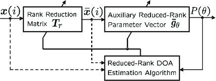
Figure 1: Proposed reduced-rank structure.

The proposed reduced-rank structure is depicted in Fig. 1. We introduce a rank-reduction matrix $\boldsymbol{T}_{r}\in\mathbb{C}^{M\times r}$, which maps the full-rank received vector $\boldsymbol{x}(i)$ into a lower dimension and generates the reduced-rank received vector $\bar{\boldsymbol{x}}(i)\in\mathbb{C}^{r\times 1}$

$$\bar{\boldsymbol{x}}(i)=\boldsymbol{T}_{r}^{H}\boldsymbol{x}(i),$$ (3)

where $\boldsymbol{T}_{r}$ consists of a collection of $r$ $M$-dimensional vectors $\boldsymbol{t}_{l}=[t_{1,l},t_{2,l},\ldots,t_{M,l}]^{T}\in\mathbb{C}^{M\times 1}$, $l=1,\ldots,r$ as given by $\boldsymbol{T}_{r}=[\boldsymbol{t}_{1},\boldsymbol{t}_{2},\ldots,\boldsymbol{t}_{r}]$, and $r$ is the rank that is assumed to be less than $M$. In what follows, all $r$ dimensional quantities are denoted with a “bar”. Compared with $\boldsymbol{x}(i)$, the dimension of $\bar{\boldsymbol{x}}(i)$ is reduced and the key features of the original signal are retained in $\bar{\boldsymbol{x}}(i)$ according to the design criterion. An auxiliary filter with the reduced-rank vector $\bar{\boldsymbol{g}}_{\theta}=[\bar{g}_{\theta,1},\bar{g}_{\theta,2},\ldots,\bar{g}_{\theta,r}]^{T}\in\mathbb{C}^{r\times 1}$ is used after the rank reduction matrix to process $\bar{\boldsymbol{x}}(i)$ to compute the output power with respect to the current scanning angle. The computational complexity is reduced if $r<<M$ for large arrays.

The rank-reduction matrix $\boldsymbol{T}_{r}$ and the auxiliary reduced-rank parameter vector $\bar{\boldsymbol{g}}_{\theta}$ are computed by the following optimization problem

$$\begin{split}&\hat{\theta}=\arg\min_{\bar{\boldsymbol{g}}_{\theta},~{}\boldsymbol{T}_{r}}~{}~{}\bar{\boldsymbol{g}}_{\theta}^{H}\boldsymbol{T}_{r}^{H}{\boldsymbol{R}}\boldsymbol{T}_{r}\bar{\boldsymbol{g}}_{\theta}\\ &\textrm{subject~{}to}~{}~{}\bar{\boldsymbol{g}}_{\theta}^{H}\boldsymbol{T}_{r}^{H}\boldsymbol{a}(\theta)=1,\end{split}$$ (4)

where ${\boldsymbol{R}}$ is the covariance matrix and the optimization problem depends on $\boldsymbol{T}_{r}$ and $\bar{\boldsymbol{g}}_{\theta}$, which have to be estimated with respect to $\theta$.

The optimization problem in (4) can be transformed by the method of Lagrange multiplier into an unconstrained one, which is

$$\mathcal{J}=\bar{\boldsymbol{g}}_{\theta}^{H}{\boldsymbol{T}}_{r}^{H}{\boldsymbol{R}}{\boldsymbol{T}}_{r}\bar{\boldsymbol{g}}_{\theta}+2~{}\mathfrak{R}~{}\big{\{}\lambda[\bar{\boldsymbol{g}}_{\theta}^{H}\boldsymbol{T}_{r}^{H}\boldsymbol{a}(\theta)-1]\big{\}},$$ (5)

where $\lambda$ is a scalar Lagrange multiplier and the operator $\mathfrak{R}(\cdot)$ selects the real part of the argument.

In order to obtain $\boldsymbol{T}_{r}$ and $\bar{\boldsymbol{g}}_{\theta}$, we make an assumption that one quantity is known and compute the other one. Specifically, assuming $\bar{\boldsymbol{g}}_{\theta}$ is known and taking the gradient of (5) with respect to $\boldsymbol{T}_{r}^{\ast}$, where $\ast$ denotes complex conjugate, we have

$$\nabla\mathcal{J}_{T_{r}^{\ast}}=\boldsymbol{R}\boldsymbol{T}_{r}\bar{\boldsymbol{g}}_{\theta}\bar{\boldsymbol{g}}_{\theta}^{H}+\lambda_{T_{r}^{\ast}}\boldsymbol{a}(\theta)\bar{\boldsymbol{g}}_{\theta}^{H}.$$ (6)

Equating the gradient to a zero matrix and solving for $\lambda_{T_{r}^{\ast}}$, the rank-reduction matrix can be expressed as

$$\boldsymbol{T}_{r}=\frac{\boldsymbol{R}^{-1}\boldsymbol{a}(\theta)}{\boldsymbol{a}^{H}(\theta)\boldsymbol{R}^{-1}\boldsymbol{a}(\theta)}\frac{\bar{\boldsymbol{g}}_{\theta}^{H}}{\|\bar{\boldsymbol{g}}_{\theta}\|^{2}},$$ (7)

where for a small number of snapshots, $\boldsymbol{R}^{-1}$ is estimated by either employing diagonal loading or the pseudo-inverse. The derivation of (7) is given in the Appendix.

Assuming that $\boldsymbol{T}_{r}$ is known and taking the gradient of (5) with respect to $\bar{\boldsymbol{g}}_{\theta}^{\ast}$, we have

$$\begin{split}\nabla\mathcal{J}_{\bar{g}_{\theta}^{\ast}}&={\boldsymbol{T}}_{r}^{H}{\boldsymbol{R}}{\boldsymbol{T}}_{r}\bar{\boldsymbol{g}}_{\theta}+\lambda_{\bar{g}_{\theta}^{\ast}}\boldsymbol{T}_{r}^{H}\boldsymbol{a}(\theta)\\ &=\bar{\boldsymbol{R}}\bar{\boldsymbol{g}}_{\theta}+\lambda_{\bar{g}_{\theta}^{\ast}}\bar{\boldsymbol{a}}(\theta),\end{split}$$ (8)

where $\bar{\boldsymbol{R}}=\mathbb{E}[\bar{\boldsymbol{x}}(i)\bar{\boldsymbol{x}}^{H}(i)]\in\mathbb{C}^{r\times r}$ is the reduced-rank covariance matrix. Setting (8) equal to a zero vector and solving for $\lambda_{\bar{g}_{\theta}^{\ast}}$, we obtain

$$\bar{\boldsymbol{g}}_{\theta}=\frac{\bar{\boldsymbol{R}}^{-1}\bar{\boldsymbol{a}}(\theta)}{\bar{\boldsymbol{a}}^{H}(\theta)\bar{\boldsymbol{R}}^{-1}\bar{\boldsymbol{a}}(\theta)},$$ (9)

where $\bar{\boldsymbol{a}}(\theta)=\boldsymbol{T}_{r}^{H}\boldsymbol{a}(\theta)\in\mathbb{C}^{r\times 1}$ is the reduced-rank steering vector with respect to the current scanning angle. A detailed derivation is included in the Appendix. Note that the auxiliary reduced-rank vector $\bar{\boldsymbol{g}}_{\theta}$ is more general for dealing with DOA estimation. Specifically, for $r=1$, the proposed JIO algorithm results in Capon’s method. For $1<r<M$, it operates under a lower dimension and thus reduces the complexity.

The output power for each scanning angle is calculated by substituting the expressions of $\boldsymbol{T}_{r}$ in (7) and $\bar{\boldsymbol{g}}_{\theta}$ in (9) into (4), which yields

$$P(\theta)=\big{(}\bar{\boldsymbol{a}}^{H}(\theta)\bar{\boldsymbol{R}}^{-1}\bar{\boldsymbol{a}}(\theta)\big{)}^{-1}.$$ (10)

By searching all possible angles, we could find peaks in the output power spectrum that correspond to the DOAs of the sources.

III-B Proposed Scheme with Polynomial Rooting

In order to avoid the exhaustive search through all possible angles, we take the polynomial rooting technique into account. Specifically, premultiplying the terms in (9) by $\bar{\boldsymbol{g}}_{\theta}^{H}$ and rearranging the terms, we have

$$Q(\theta)=\bar{\boldsymbol{a}}^{H}(\theta)\bar{\boldsymbol{R}}^{-1}\bar{\boldsymbol{a}}(\theta)=\frac{\bar{\boldsymbol{g}}_{\theta}^{H}\bar{\boldsymbol{R}}^{-1}\bar{\boldsymbol{a}}(\theta)}{\|\bar{\boldsymbol{g}}_{\theta}\|^{2}},$$ (11)

where $Q(\theta)=P^{-1}(\theta)$.

The proposed reduced-rank scheme performs DOA estimation by scanning a limited range of angles without an exhaustive search. Compared with (10), the expression in (11) brings a simplification in the joint optimization of the rank-reduction matrix and the auxiliary reduced-rank parameter vector. We show the advantage of this scheme in the simulations. Note that, in this paper, the objective of the application of the polynomial rooting is not only an extension of the proposed scheme. It is viewed as an approach to reduce the computational complexity.

Another effective technique that could be employed in the proposed scheme is beamspace preprocessing [4, pp. 1243-1251], [36], which preprocesses the received vector with a matrix that, in essence, creates a set of beams. It reduces the complexity from the number of sensor elements to the number of beams utilized to probe a given sector. We then use these beam outputs to estimate the DOAs. In many environments, DOA estimation with the beamspace preprocessing achieves an improved probability of resolution with substantially less computational complexity. Furthermore, numerous works have been reported to combine polynomial rooting and beamspace techniques into one scheme for robustness [37], [38]. In the proposed reduced-rank scheme, it is possible to consider the beamspace technique as an extension of the current work for improving the resolution and reducing the complexity.

IV Proposed Reduced-Rank Algorithms

In this section, we derive a constrained LS algorithm for an implementation of the proposed reduced-rank scheme. The proposed algorithm jointly estimates the rank-reduction matrix and auxiliary reduced-rank parameter vector using an alternating optimization procedure. The rank is selected via the model order selection approach. The FBA technique is employed in the algorithm to deal with highly correlated sources for the resolution improvement. We utilize the matrix inversion lemma to develop a recursive least squares (RLS) based algorithm for DOA estimation. With these algorithms a designer can choose between batch or adaptive (recursive) processing. In particular, adaptive techniques can be used if a designer is interested in reducing the computational cost per snapshot as compared to computing a matrix inversion. In batch processing a designer needs to compute a matrix inversion, which might be a choice for a stationary scenario that only requires one matrix inversion.

IV-A Proposed JIO Algorithm

From (7) and (9), the challenge left to us is how to efficiently compute the rank-reduction matrix $\boldsymbol{T}_{r}$ and the auxiliary reduced-rank vector $\bar{\boldsymbol{g}}_{\theta}$ for solving (4). Using the method of LS, the constraint in (4) can be incorporated by the method of Lagrange multipliers in the form

$$\mathcal{J}_{\textrm{LS}}=\sum_{l=1}^{i}\alpha^{i-l}|\bar{\boldsymbol{g}}_{\theta}^{H}(i)\boldsymbol{T}_{r}^{H}(i)\boldsymbol{x}(l)|^{2}+2~{}\mathfrak{R}\big{\{}\lambda\big{[}\bar{\boldsymbol{g}}_{\theta}^{H}(i)\boldsymbol{T}_{r}^{H}(i)\boldsymbol{a}(\theta)-1\big{]}\big{\}},$$ (12)

where $\alpha$ is a forgetting factor that is a positive constant close to, but less than $1$. Assuming $\bar{\boldsymbol{g}}_{\theta}(i)$ is known, taking the gradient of (12) with respect to $\boldsymbol{T}_{r}^{\ast}(i)$ yields,

$$\begin{split}{\nabla\mathcal{J}_{\textrm{LS}_{T_{r}^{\ast}}}}&=\sum_{l=1}^{i}\alpha^{i-l}\boldsymbol{x}(l)\boldsymbol{x}^{H}(l)\boldsymbol{T}_{r}(i)\bar{\boldsymbol{g}}_{\theta}(i)\bar{\boldsymbol{g}}_{\theta}^{H}(i)+\lambda_{T_{r}^{\ast}}\boldsymbol{a}(\theta)\bar{\boldsymbol{g}}_{\theta}^{H}(i)\\ &=\hat{\boldsymbol{R}}(i)\boldsymbol{T}_{r}(i)\bar{\boldsymbol{g}}_{\theta}(i)\bar{\boldsymbol{g}}^{H}(\theta)(i)+\lambda_{T_{r}^{\ast}}\boldsymbol{a}(\theta)\bar{\boldsymbol{g}}_{\theta}^{H}(i),\end{split}$$ (13)

where $\hat{\boldsymbol{R}}(i)=\sum_{l=1}^{i}\alpha^{i-l}\boldsymbol{x}(l)\boldsymbol{x}^{H}(l)\in\mathbb{C}^{M\times M}$ is an estimate of the covariance matrix at time instant $i$ and can be written in a recursive form $\hat{\boldsymbol{R}}(i)=\alpha\hat{\boldsymbol{R}}(i-1)+\boldsymbol{x}(i)\boldsymbol{x}^{H}(i)$.

The resulting rank-reduction matrix is

$$\boldsymbol{T}_{r}(i)=\frac{\hat{\boldsymbol{R}}^{-1}(i)\boldsymbol{a}(\theta)}{\boldsymbol{a}^{H}(\theta)\hat{\boldsymbol{R}}^{-1}(i)\boldsymbol{a}(\theta)}\frac{\bar{\boldsymbol{g}}_{\theta}^{H}(i)}{\|\bar{\boldsymbol{g}}_{\theta}(i)\|^{2}}.$$ (14)

Fixing $\boldsymbol{T}_{r}(i)$, taking the gradient of (12) with respect to $\bar{\boldsymbol{g}}_{\theta}^{\ast}(i)$, it becomes

$$\begin{split}\nabla\mathcal{J}_{\textrm{LS}_{\bar{g}_{\theta}^{\ast}}}&=\sum_{l=1}^{i}\alpha^{i-l}\boldsymbol{T}_{r}^{H}(i)\boldsymbol{x}(l)\boldsymbol{x}^{H}(l)\boldsymbol{T}_{r}(i)\bar{\boldsymbol{g}}_{\theta}(i)+\lambda_{\bar{g}_{\theta}^{\ast}}\boldsymbol{T}_{r}^{H}(i)\boldsymbol{a}(\theta)\\ &=\hat{\bar{\boldsymbol{R}}}(i)\bar{\boldsymbol{g}}_{\theta}(i)+\lambda_{\bar{g}_{\theta}^{\ast}}\boldsymbol{T}_{r}^{H}(i)\boldsymbol{a}(\theta),\end{split}$$ (15)

where $\hat{\bar{\boldsymbol{R}}}(i)=\sum_{l=1}^{i}\alpha^{i-l}\bar{\boldsymbol{x}}(l)\bar{\boldsymbol{x}}^{H}(l)\in\mathbb{C}^{r\times r}$ is an estimate of the reduced-rank covariance matrix. Its recursive form is $\hat{\bar{\boldsymbol{R}}}(i)=\alpha\hat{\bar{\boldsymbol{R}}}(i-1)+\bar{\boldsymbol{x}}(i)\bar{\boldsymbol{x}}^{H}(i)$. The resulting expression of $\bar{\boldsymbol{g}}_{\theta}(i)$ is

$$\bar{\boldsymbol{g}}_{\theta}(i)=\frac{\hat{\bar{\boldsymbol{R}}}^{-1}(i)\bar{\boldsymbol{a}}(\theta)}{\bar{\boldsymbol{a}}^{H}(\theta)\hat{\bar{\boldsymbol{R}}}^{-1}(i)\bar{\boldsymbol{a}}(\theta)}.$$ (16)

Note that the expression of the rank-reduction matrix in (14) is a function of $\bar{\boldsymbol{g}}_{\theta}(i)$ while the auxiliary reduced-rank vector obtained from (16) depends on $\boldsymbol{T}_{r}(i)$. The proposed algorithm relies on an iterative exchange of information between $\boldsymbol{T}_{r}(i)$ and $\bar{\boldsymbol{g}}_{\theta}(i)$, which results in an improved convergence performance. The proposed JIO algorithm is summarized in Table I, where $\hat{\bar{\boldsymbol{R}}}$ is the estimate of the reduced-rank correlation matrix related to $N$ snapshots, the scanning angle $\theta_{n}=n\triangle^{o}$, $\triangle^{o}$ is the search step, and $n=1,2,\ldots,180^{o}/\triangle^{o}$. For a simple and convenient search, we make $180^{o}/\triangle^{o}$ an integer. It is necessary to initialize $\boldsymbol{T}_{r}(0)$ to start the update due to the dependence between $\boldsymbol{T}_{r}(i)$ and $\bar{\boldsymbol{g}}_{\theta}(i)$, see Table I.

The output power $P(\theta_{n})$ is much higher if the scanning angle $\theta_{n}=\theta_{k}$, ($k=0,\ldots,q-1$), which corresponds to the position of the source, compared with other scanning angles with respect to the noise level. Thus, we can estimate the DOAs by finding the peaks in the output power spectrum. We refer to [4, pp.1142-1146] for the individual computational costs of the recursions.

TABLE I: The proposed JIO algorithm

Initialization:

$\boldsymbol{T}_{r}(0)=[\boldsymbol{I}_{r\times r}^{T}~{}{\boldsymbol{0}_{(M-r)\times r}^{T}}]^{T}$

Update for each time instant $i=1,\ldots,N$

$\bar{\boldsymbol{x}}(i)=\boldsymbol{T}_{r}^{H}(i-1)\boldsymbol{x}(i)$

$\bar{\boldsymbol{a}}(\theta_{n})=\boldsymbol{T}_{r}^{H}(i-1)\boldsymbol{a}(\theta_{n})$

$\hat{{\boldsymbol{R}}}(i)=\alpha\hat{{\boldsymbol{R}}}(i-1)+{\boldsymbol{x}}(i){\boldsymbol{x}}^{H}(i)$

$\hat{\bar{\boldsymbol{R}}}(i)=\alpha\hat{\bar{\boldsymbol{R}}}(i-1)+\bar{\boldsymbol{x}}(i)\bar{\boldsymbol{x}}^{H}(i)$

$\bar{\boldsymbol{g}_{\theta}}(i)={\hat{\bar{\boldsymbol{R}}}^{-1}(i)\bar{\boldsymbol{a}}(\theta_{n})}/\big{(}{\bar{\boldsymbol{a}}^{H}(\theta_{n})\hat{\bar{\boldsymbol{R}}}^{-1}(i)\bar{\boldsymbol{a}}(\theta_{n})}\big{)}$

$\boldsymbol{T}_{r}(i)=\frac{\hat{\boldsymbol{R}}^{-1}(i)\boldsymbol{a}(\theta_{n})}{\boldsymbol{a}^{H}(\theta_{n})\hat{\boldsymbol{R}}^{-1}(i)\boldsymbol{a}(\theta_{n})}\frac{\bar{\boldsymbol{g}_{\theta}}^{H}(i)}{\|\bar{\boldsymbol{g}_{\theta}}(i)\|^{2}}$

Output power

$P(\theta_{n})=1/\big{(}\bar{\boldsymbol{a}}^{H}(\theta_{n})\hat{\bar{\boldsymbol{R}}}^{-1}\bar{\boldsymbol{a}}(\theta_{n})\big{)}$

Polynomial rooting (optional)

$Q(\theta)=\bar{\boldsymbol{a}}^{H}(\theta)\bar{\boldsymbol{R}}^{-1}\bar{\boldsymbol{a}}(\theta)$

IV-B Proposed JIO Algorithm with FBA

The FBA technique is helpful to increase the resolution for DOA estimation when the sources are correlated. It is based on the averaging of the covariance matrix of identical overlapping arrays and so requires an array of identical elements equipped with some form of periodic structure, such as the ULA. For its application, we split a ULA antenna array into a set of forward and conjugate backward subarrays. The FBA preprocessing operates on $\boldsymbol{x}(i)$ to estimate the forward and backward subarray covariance matrices that are averaged to get the forward/conjugate backward smoothed covariance matrix. The JIO algorithm incorporated with the FBA technique is termed JIO(FBA).

In this work, we employ an efficient way to estimate the forward/conjugate backward covariance matrix (see Eq. (3.22) in [34]). The resulting JIO(FBA) algorithm is summarized in Table II, where $\boldsymbol{\Pi}_{M}\in\mathbb{C}^{M\times M}$ is a matrix with ones on its antidiagonal and zeros elsewhere, $\hat{\boldsymbol{R}}_{\textrm{fb}}(i)$ and $\hat{\bar{\boldsymbol{R}}}_{\textrm{fb}}(i)$ are the full-rank and the reduced-rank forward/backward averaged covariance matrices, respectively. Note that $\hat{\boldsymbol{R}}(i)$ here is calculated by using a time-averaged estimate, i.e., $\hat{{\boldsymbol{R}}}(i)=\alpha\hat{{\boldsymbol{R}}}(i-1)+{\boldsymbol{x}}(i){\boldsymbol{x}}^{H}(i)$. The proposed JIO(FBA) algorithm employs the averaged $\hat{\boldsymbol{R}}_{\textrm{fb}}(i)$ and $\hat{\bar{\boldsymbol{R}}}_{\textrm{fb}}(i)$ to compute $\bar{\boldsymbol{g}}_{\theta,\textrm{fb}}(i)$ and $\boldsymbol{T}_{\textrm{fb}}(i)$ for the output power with respect to each scanning angle $\theta_{n}$. The computational complexity can be significantly reduced by using a real-valued implementation [34].

TABLE II: The proposed JIO(FBA) algorithm

Initialization:

$\boldsymbol{T}_{\textrm{fb}}(0)=[\boldsymbol{I}_{r\times r}^{T}~{}{\boldsymbol{0}_{(M-r)\times r}^{T}}]^{T}$

Update for each time instant $i=1,\ldots,N$

$\bar{\boldsymbol{a}}_{\textrm{fb}}(\theta_{n})=\boldsymbol{T}_{\textrm{fb}}^{H}(i-1)\boldsymbol{a}(\theta_{n})$

$\hat{{\boldsymbol{R}}}(i)=\alpha\hat{{\boldsymbol{R}}}(i-1)+{\boldsymbol{x}}(i){\boldsymbol{x}}^{H}(i)$

$\hat{\boldsymbol{R}}_{\textrm{fb}}(i)=\frac{1}{2}\big{[}\hat{\boldsymbol{R}}(i)+\boldsymbol{\Pi}_{M}\hat{\boldsymbol{R}}^{\ast}(i)\boldsymbol{\Pi}_{M}\big{]}$

$\hat{\bar{\boldsymbol{R}}}_{\textrm{fb}}(i)=\boldsymbol{T}_{\textrm{fb}}^{H}(i-1)\hat{\boldsymbol{R}}_{\textrm{fb}}(i)\boldsymbol{T}_{\textrm{fb}}(i-1)$

$\bar{\boldsymbol{g}}_{{\theta},\textrm{fb}}(i)={\hat{\bar{\boldsymbol{R}}}_{\textrm{fb}}^{-1}(i)\bar{\boldsymbol{a}}_{\textrm{fb}}(\theta_{n})}/\big{(}{\bar{\boldsymbol{a}}_{\textrm{fb}}^{H}(\theta_{n})\hat{\bar{\boldsymbol{R}}}_{\textrm{fb}}^{-1}(i)\bar{\boldsymbol{a}}_{\textrm{fb}}(\theta_{n})}\big{)}$

$\boldsymbol{T}_{\textrm{fb}}(i)=\frac{\hat{\boldsymbol{R}}_{\textrm{fb}}^{-1}(i)\boldsymbol{a}(\theta_{n})}{\boldsymbol{a}^{H}(\theta_{n})\hat{\boldsymbol{R}}_{\textrm{fb}}^{-1}(i)\boldsymbol{a}(\theta_{n})}\frac{\bar{\boldsymbol{g}}_{{\theta},{\textrm{fb}}}^{H}(i)}{\|\bar{\boldsymbol{g}}_{{\theta},{\textrm{fb}}}(i)\|^{2}}$

Output power

$P(\theta_{n})=1/\big{(}\bar{\boldsymbol{a}}_{\textrm{fb}}^{H}(\theta_{n})\hat{\bar{\boldsymbol{R}}}_{\textrm{fb}}^{-1}\bar{\boldsymbol{a}}_{\textrm{fb}}(\theta_{n})\big{)}$

Polynomial rooting (optional)

$Q(\theta)=\bar{\boldsymbol{a}}^{H}(\theta)\bar{\boldsymbol{R}}^{-1}\bar{\boldsymbol{a}}(\theta)$

IV-C Proposed JIO-RLS Algorithm

We utilize the matrix inversion lemma [31] to develop a JIO-based RLS algorithm (JIO-RLS) for DOA estimation without the matrix inverse. Specifically, defining $\hat{\boldsymbol{\Phi}}(i)=\hat{\boldsymbol{R}}^{-1}(i)$, yields

$$\boldsymbol{k}(i)=\frac{\alpha^{-1}\hat{\boldsymbol{\Phi}}(i-1)\boldsymbol{x}(i)}{1+\alpha^{-1}\boldsymbol{x}^{H}(i)\hat{\boldsymbol{\Phi}}(i-1)\boldsymbol{x}(i)},$$ (17)

$$\hat{\boldsymbol{\Phi}}(i)=\alpha^{-1}\hat{\boldsymbol{\Phi}}(i-1)-\alpha^{-1}\boldsymbol{k}(i)\boldsymbol{x}^{H}(i)\hat{\boldsymbol{\Phi}}(i-1),$$ (18)

where $\boldsymbol{k}(i)\in\mathbb{C}^{M\times 1}$ is the Kalman gain vector and $\hat{\boldsymbol{\Phi}}(0)=\delta\boldsymbol{I}_{M\times M}$ with $\delta$ being a positive value that needs to be set for numerical stability.

Given $\hat{\bar{\boldsymbol{\Phi}}}(i)=\hat{\bar{\boldsymbol{R}}}^{-1}(i)$, we have

$$\bar{\boldsymbol{k}}(i)=\frac{\alpha^{-1}\hat{\bar{\boldsymbol{\Phi}}}(i-1)\bar{\boldsymbol{x}}(i)}{1+\alpha^{-1}\bar{\boldsymbol{x}}^{H}(i)\hat{\bar{\boldsymbol{\Phi}}}(i-1)\bar{\boldsymbol{x}}(i)},$$ (19)

$$\hat{\bar{\boldsymbol{\Phi}}}(i)=\alpha^{-1}\hat{\bar{\boldsymbol{\Phi}}}(i-1)-\alpha^{-1}\bar{\boldsymbol{k}}(i)\bar{\boldsymbol{x}}^{H}(i)\hat{\bar{\boldsymbol{\Phi}}}(i-1),$$ (20)

where $\bar{\boldsymbol{k}}(i)\in\mathbb{C}^{r\times 1}$ is the reduced-rank gain vector and $\hat{\bar{\boldsymbol{\Phi}}}(0)=\bar{\delta}\boldsymbol{I}_{r\times r}$ with $\bar{\delta}>0$.

Substituting the recursive procedures (17)-(20) into the proposed JIO algorithm instead of the matrix inverse results in the JIO-RLS algorithm, which is concluded in Table III, where $\delta$ and $\bar{\delta}$ are selected according to the input signal-to-noise ratio (SNR) [31], and $\hat{\boldsymbol{\Phi}}$ is the estimate of the inverse of the received covariance matrix after $N$ snapshots. The specific values will be given in the simulations. The JIO-RLS algorithm retains the positive feature of the iterative exchange of information between the rank-reduction matrix and auxiliary reduced-rank vector, which avoids the degradation of the resolution, and utilizes a recursive procedure to compute $\hat{\boldsymbol{R}}^{-1}$ and $\hat{\bar{\boldsymbol{R}}}^{-1}$ for the reduced complexity.

TABLE III: Proposed JIO-RLS algorithm

Initialization:

$\boldsymbol{T}_{r}(0)=[\boldsymbol{I}_{r}^{T}~{}{\boldsymbol{0}_{(M-r)\times r}^{T}}]^{T}$;   $\delta,~{}\bar{\delta}=$positive constants;

$\hat{\boldsymbol{\Phi}}(0)=\delta\boldsymbol{I}_{M\times M}$;   $\hat{\bar{\boldsymbol{\Phi}}}(0)=\bar{\delta}\boldsymbol{I}_{r\times r}$.

Update for each time instant $i=1,\ldots,N$

$\bar{\boldsymbol{x}}(i)=\boldsymbol{T}_{r}^{H}(i-1)\boldsymbol{x}(i)$

$\bar{\boldsymbol{a}}(\theta_{n})=\boldsymbol{T}_{r}^{H}(i-1)\boldsymbol{a}(\theta_{n})$

$\bar{\boldsymbol{k}}(i)=\frac{\alpha^{-1}\hat{\bar{\boldsymbol{\Phi}}}(i-1)\bar{\boldsymbol{x}}(i)}{1+\alpha^{-1}\bar{\boldsymbol{x}}^{H}(i)\hat{\bar{\boldsymbol{\Phi}}}(i-1)\bar{\boldsymbol{x}}(i)}$

$\hat{\bar{\boldsymbol{\Phi}}}(i)=\alpha^{-1}\hat{\bar{\boldsymbol{\Phi}}}(i-1)-\alpha^{-1}\bar{\boldsymbol{k}}(i)\bar{\boldsymbol{x}}^{H}(i)\hat{\bar{\boldsymbol{\Phi}}}(i-1)$

$\bar{\boldsymbol{g}}_{\theta}(i)=\frac{\hat{\bar{\boldsymbol{\Phi}}}(i)\bar{\boldsymbol{a}}(\theta_{n})}{\bar{\boldsymbol{a}}^{H}(\theta_{n})\hat{\bar{\boldsymbol{\Phi}}}(i)\bar{\boldsymbol{a}}(\theta_{n})}$

$k(i)=\frac{\alpha^{-1}\hat{\boldsymbol{\Phi}}(i-1)\boldsymbol{x}(i)}{1+\alpha^{-1}\boldsymbol{x}^{H}(i)\hat{\boldsymbol{\Phi}}(i-1)\boldsymbol{x}(i)}$

$\hat{\boldsymbol{\Phi}}(i)=\alpha^{-1}\hat{\boldsymbol{\Phi}}(i-1)-\alpha^{-1}\boldsymbol{k}(i)\boldsymbol{x}^{H}(i)\hat{\boldsymbol{\Phi}}(i-1)$

$\boldsymbol{T}_{r}(i)=\frac{\hat{\boldsymbol{\Phi}}(i)\boldsymbol{a}(\theta_{n})}{\boldsymbol{a}(\theta_{n})^{H}\hat{\boldsymbol{\Phi}}(i)\boldsymbol{a}(\theta_{n})}\frac{\bar{\boldsymbol{g}}_{\theta}^{H}(i)}{\|\bar{\boldsymbol{g}}_{\theta}(i)\|^{2}}$

Output power

$P(\theta_{n})=1/\big{(}\bar{\boldsymbol{a}}^{H}(\theta_{n})\hat{\bar{\boldsymbol{\Phi}}}\bar{\boldsymbol{a}}(\theta_{n})\big{)}$

Polynomial rooting (optional)

$Q(\theta)=\bar{\boldsymbol{a}}^{H}(\theta)\bar{\boldsymbol{R}}^{-1}\bar{\boldsymbol{a}}(\theta)$

We can also use the FBA technique in the proposed JIO-RLS algorithm to improve the resolution when the sources are correlated. The full-rank and the reduced-rank forward/conjugate backward smoothed covariance matrix can be estimated by $\hat{\boldsymbol{R}}_{\textrm{fb}}(i)$ and $\hat{\bar{\boldsymbol{R}}}_{\textrm{fb}}(i)$ in Table II. Using the matrix inversion lemma for the calculation of $\hat{\boldsymbol{\Phi}}_{\textrm{fb}}(i)=\hat{\boldsymbol{R}}_{\textrm{fb}}^{-1}(i)$ and $\hat{\bar{\boldsymbol{\Phi}}}_{\textrm{fb}}(i)=\hat{\bar{\boldsymbol{R}}}_{\textrm{fb}}^{-1}(i)$, we have

$$\begin{split}&\hat{\boldsymbol{\Phi}}_{\textrm{fb}}(i)=2[\hat{\boldsymbol{\Phi}}(i)-\frac{\hat{\boldsymbol{\Phi}}(i)\boldsymbol{\Pi}_{M}\Pi_{M}^{H}\hat{\boldsymbol{\Phi}}(i)}{\hat{\boldsymbol{\Phi}}^{\ast}(i)+\boldsymbol{\Pi}_{M}^{H}\hat{\boldsymbol{\Phi}}(i)\boldsymbol{\Pi}_{M}}]\\ &\hat{\bar{\boldsymbol{\Phi}}}_{\textrm{fb}}(i)=2[\hat{\bar{\boldsymbol{\Phi}}}(i)-\frac{\hat{\bar{\boldsymbol{\Phi}}}(i)\boldsymbol{T}_{\textrm{fb}}^{H}(i-1)\boldsymbol{\Pi}_{M}\Pi_{M}^{H}\boldsymbol{T}_{\textrm{fb}}(i-1)\hat{\bar{\boldsymbol{\Phi}}}(i)}{\hat{\bar{\boldsymbol{\Phi}}}^{\ast}(i)+\boldsymbol{\Pi}_{M}^{H}\boldsymbol{T}_{\textrm{fb}}(i-1)\hat{\bar{\boldsymbol{\Phi}}}(i)\boldsymbol{T}_{\textrm{fb}}^{H}(i-1)\boldsymbol{\Pi}_{M}}],\end{split}$$

where both $\hat{\boldsymbol{\Phi}}(i)$ and $\hat{\bar{\boldsymbol{\Phi}}}(i)$ are calculated by their recursive expressions, which have been given in Table III. By using $\hat{\boldsymbol{\Phi}}_{\textrm{fb}}(i)$ and $\hat{\bar{\boldsymbol{\Phi}}}_{\textrm{fb}}(i)$ to replace $\hat{\boldsymbol{\Phi}}(i)$ and $\hat{\bar{\boldsymbol{\Phi}}}(i)$ in Table III, respectively, for calculating the rank-reduction matrix and the auxiliary reduced-rank parameter vector, we can compute the output power with respect to each scanning angle and find the DOAs corresponding to the sources.

We have so far detailed the proposed reduced-rank scheme and the derivations of the proposed algorithms. There are two points that need to be interpreted here. First, the polynomial rooting technique derived in Section III-B can be employed in the proposed algorithms as a preprocessing step to save the computational cost. Second, the proposed JIO algorithms could work without the exact knowledge of the number of sources $q$. They jointly update the rank-reduction matrix and auxiliary reduced-rank vector to calculate the output power and scan possible angles to plot the output power spectrum, which do not require information about $q$. Most existing algorithms need this information since, for the subspace-based algorithms, $q$ is critical to construct the signal subspace, and, for the ML algorithm, it is important to improve the resolution. However, $q$ has to be estimated using other techniques with more complex procedures, which increase the computational cost.

IV-D Model-Order Selection

The selection of the rank $r$ is important to the proposed algorithms since it determines how much information could be retained in the reduced-rank received vector and thus impacts the resolution. However, it does not mean that a larger $r$ always leads to a better resolution. A large $r$ (e.g., close to $M$) increases the dimension of the reduced-rank received vector, which may cause redundancy and significantly increase the computational complexity. On the other hand, a small $r$ saves the cost but may lose information that is useful to improve the resolution. In most of the existing subspace algorithms, $r$ equals $q$, which is employed in the eigen-decomposition for the construction of the signal subspace. In the proposed algorithms, $r$ could be set to be some specific values that do not necessarily equal $q$. The range of values has been obtained by experiments and the theoretical explanation is that the subspace fitting performed by the JIO algorithms does not require many bases in the subspace to result in a good performance. This has been verified in the simulations.

We introduce an adaptive approach for selecting the rank. We describe a model-order selection method based on the MV criterion computed by the rank-reduction matrix $\boldsymbol{T}_{r}^{(r)}$ and the auxiliary reduced-rank parameter vector $\bar{\boldsymbol{g}}^{(r)}$, which is

$$\begin{split}&\boldsymbol{T}_{r}^{(r)}=\begin{bmatrix}t_{1,1}&t_{1,2}&\ldots&t_{1,r_{\textrm{min}}}&\ldots&t_{1,r_{\textrm{max}}}\\ t_{2,1}&t_{2,2}&\ldots&t_{2,r_{\textrm{min}}}&\ldots&t_{2,r_{\textrm{max}}}\\ \vdots&\vdots&\vdots&\vdots&\vdots&\vdots\\ t_{M,1}&t_{M,2}&\ldots&t_{M,r_{\textrm{min}}}&\ldots&t_{M,r_{\textrm{max}}}\\ \end{bmatrix},\\ &\bar{\boldsymbol{g}}_{\theta}^{(r)}=\begin{bmatrix}\bar{g}_{1}&\bar{g}_{2}&\ldots&\bar{g}_{r_{\textrm{min}}}&\ldots&\bar{g}_{r_{\textrm{max}}}\\ \end{bmatrix}^{T},\end{split}$$ (21)

where the superscript $(\cdot)^{(r)}$ denotes the rank used for the adaptation at each time instant, $r_{\textrm{min}}$ and $r_{\textrm{max}}$ are the minimum and maximum ranks allowed, respectively.

The rank is adopted automatically based on the exponentially-weighted a posteriori MV criterion used to derive the rank-reduction matrix and the auxiliary reduced-rank vector, which is

$$\begin{split}&\mathcal{J}_{\textrm{PLS}}\big{(}\boldsymbol{T}_{r}^{(r)}(i-1),\bar{\boldsymbol{g}}^{(r)}(i-1)\big{)}=\\ &~{}~{}~{}~{}~{}~{}~{}~{}~{}~{}\sum_{l=1}^{i}\varrho^{i-l}|\bar{\boldsymbol{g}}_{\theta}^{(r)H}(i-1)\boldsymbol{T}_{r}^{(r)H}(i-1)\boldsymbol{x}(l)|^{2},\end{split}$$ (22)

where $\varrho$ is the exponential weight factor that is required as the optimal rank $r$ can change as a function of the time instant $i$. For each time instant, $\boldsymbol{T}_{r}^{(r)}(i)$ and $\bar{\boldsymbol{g}}_{\theta}^{(r)}(i)$ are computed for a selected $r$ according to (22). The developed model-order selection method is given by

$$r_{\textrm{opt}}=\textrm{arg}\min_{r_{\textrm{min}}\leq r\leq r_{\textrm{max}}}\mathcal{J}_{\textrm{PLS}}\big{(}\boldsymbol{T}_{r}^{(r)}(i-1),\bar{\boldsymbol{g}}_{\theta}^{(r)}(i-1)\big{)},$$ (23)

where $r$ is an integer ranging between $r_{\textrm{min}}$ and $r_{\textrm{max}}$. For each $\theta_{n}$, we calculate $\boldsymbol{T}_{r}^{(r)}$ and $\bar{\boldsymbol{g}}_{\theta}^{(r)}$ until $r=r_{\textrm{max}}$, and then scan $(r)$ from $r_{\textrm{min}}$ to $r_{\textrm{max}}$ to find a pair of $\{\boldsymbol{T}_{r}^{(r)},\bar{\boldsymbol{g}}_{\theta}^{(r)}\}$ that satisfy (23). It should be noted that the model-order selection algorithm is not very expensive because it re-uses entries of the rank-reduction matrix which is initially computed with $r_{\rm max}$ and the matrix inverse (no extra matrix inverse is required). The algorithm then computes extra terms for the optimization in (23). The corresponding $(r)$ is the most appropriate value with respect to the current time instant. We found that the range for which the rank $r$ has an impact on the resolution is very limited, being from $r_{\textrm{min}}=3$ to $r_{\textrm{max}}=7$. These values are rather insensitive to the number of users in the system, to the number of sensor elements, and work effectively for the studied scenarios. If $q$ is larger than $r_{m}ax$ then there is a potential risk of undermodelling. However, the method proposed concentrates the energy of the subspace in a different way as compared to an eigen-based technique. This is the reason why it was found that $r_{m}ax=7$ was enough for the scenarios studied. Alternatively, an additional mechanism can be used to adjust $r_{\textrm{min}}$ and $r_{\textrm{max}}$. The model-order selection procedure involves additional complexity corresponding to the computation of the cost function in (23) and requires $3(r_{\rm max}-r_{\rm min})+1$ additions and a sorting algorithm to find the best model order according to (23). It is efficient to combine this approach with the polynomial rooting technique to select the most appropriate rank for the proposed algorithms.

IV-E Complexity Analysis

Considering the computational cost, Capon’s method, MUSIC, and ESPRIT work with $O(M^{3})$ due to the matrix inverse and the eigen-decomposition, respectively. The recent AV and CG algorithms pay a higher cost [14] due to the generation of the signal subspace. The API subspace tracking approach estimates the signal subspace of the MUSIC and the ESPRIT with lower complexity $O(qM+q^{3})$. However, its complexity becomes relatively high as the number of sources $q$ becomes large. For the proposed algorithms, the JIO algorithm requires $O(M^{3}+r^{3})$ due to the matrix inverse. The JIO-RLS algorithm requires $O(M^{2}+r^{2})$ due to the use of the matrix inversion lemma [31]. It is worth noting that the cost of computing $\hat{\boldsymbol{\Phi}}$ is saved after the procedure of the first scanning angle since it is invariable for the rest of the search.

We provide a comparison of the computational complexity for the proposed and existing algorithms in Table IV, where $M$ denotes the number of sensor elements, $q$ is the number of sources, $\Delta$ is the search step, $D$ is the iteration number for the CG algorithm, and $r$ is the rank. Note that the cost of $r^{3}$ (or $r^{2}$) is much less than that of $M^{3}$ (or $M^{2}$) since $r$ is always much smaller than $M$ for sufficiently large arrays. Our studies reveal that the range for which the rank $r$ has a positive impact on the performance is limited among a set of small values. This fact has been referred to the previous section and will be verified in the simulations. The complexity of the algorithms equipped via the FBA technique is not shown in this table since it is viewed as a preprocessing step and requires nearly the same cost for all the methods.

TABLE IV: Comparison of The Computational Complexity

Algorithms	Complexity	Main Procedures
Capon	$O(M^{3})$	Matrix inverse (grid search)
MUSIC	$O(M^{3})$	Eigen-decomposition (grid search)
MUSIC(API)	$O(qM+q^{3})$	Subspace tracking (grid search)
ESPRIT	$O(M^{3})$	Eigen-decomposition
ESPRIT(API)	$O(qM+q^{3})$	Subspace tracking
AV	$O((180/\Delta)qM^{2})$	Construction of signal subspace (grid search)
CG	$O((180/\Delta)DM^{2})$	Construction of signal subspace (grid search)
JIO	$O(M^{3}+(180/\Delta)r^{3})$	Matrix inverse and reduced-rank process (grid search)
JIO-RLS	$O(M^{2}+(180/\Delta)r^{2})$	Matrix inversion lemma and reduced-rank processing (grid search)
Root JIO-RLS	$O(M^{2}+r^{2})$	Matrix inversion lemma and reduced-rank processing (polynomial rooting)

V Simulations

In this section, we evaluate the probability of resolution of the proposed JIO algorithms and compare them with a number of existing DOA estimation algorithms. The probability of resolution for two sources is defined as $P_{r}[|\hat{\theta}_{1}-\theta_{1}|{\rm and}|\hat{\theta}_{2}-\theta_{2}|<|\theta_{1}-\theta_{2}|/2]$ [13], [41]. We compare the proposed JIO algorithms with Capon’s method, the MUSIC and ESPRIT subspace-based methods with and without the API subspace tracking implementation, the projected companion matrix MUSIC (PCM-MUSIC) [16], the fast root MUSIC [9] and the ML method. In all simulations, binary phase shift keying (BPSK) sources separated by $3^{o}$ with powers $\sigma_{s}^{2}=1$ are considered and the noise is spatially and temporally white Gaussian. All the results are averaged over $1000$ runs. The search step is $\Delta^{o}=0.5^{o}$. The forgetting factor $\alpha$ corresponds to a coherence window of $1/(1-\alpha)$ snapshots. When the number of snapshots is small which is the case of interest in this work, then there is no significant impact of using an $\alpha$ different from $1$ but as the number of snapshots is increased the forgetting factor should match the coherence window of the time-varying process in order to track dynamic sources. The forgetting factor is important in non-stationary scenarios in which there is need to discard past data to obtain more accurate estimates. The diagonal loading (or regularization) has been used for all the methods and the parameters have been optimized for each method in order to ensure a fair comparison. Simulations are performed for a ULA with half a wavelength inter-element spacing for a generic application of all studied algorithms.

In Fig. 2, we assess the impact of the correlated sources on the performance of the proposed and existing algorithms. The array size is $M=40$ and the number of snapshots $N=10$ is fixed. There are $q=2$ highly correlated sources in the system with correlation value $\tau=0.9$, which are generated as follows [13]:

$$s_{1}\sim\mathcal{N}(0,\sigma_{s}^{2})~{}~{}\textrm{and}~{}~{}s_{2}=\tau s_{1}+\sqrt{1-\tau^{2}}s_{3},$$

where $s_{3}\sim\mathcal{N}(0,\sigma_{s}^{2})$. The rank for the proposed JIO algorithm is $r=4$. We have verified the rank among $r\in[1,8]$ and found that $r=4$ is the most appropriate value. Although the values that are higher than $r=4$ could also achieve a relatively high probability of resolution, they result in a higher computational load if $r\rightarrow M$. The probability of resolution is plotted against the input SNR values. From Fig. 2, we can see that the ML algorithm is superior to the other analyzed algorithms. However, it requires a higher computational cost than the remaining techniques. The proposed JIO algorithm outperforms other existing algorithms for different SNR values.

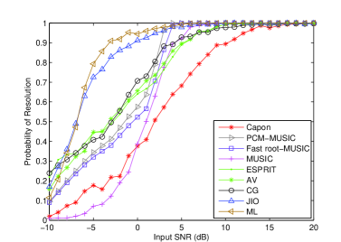
Figure 2: Probability of resolution versus input SNR with $\alpha=0998$, $M=40$, $N=10$, $q=2$, $\tau=0.9$, $r_{\rm opt}=4$.

In Fig. 3, we consider the same scenario as in Fig. 2 and show the performance of the proposed and existing algorithms equipped with the FBA technique. The ML algorithm is included in this experiment to provide a comparison with Fig. 2. It is clear that the FBA technique is useful to the studied algorithms for dealing with the problem of the highly correlated sources. The probability of resolution for each algorithm is improved under this case in comparison with its conventional counterpart shown in Fig. 2. The proposed JIO algorithm shows a high performance that is close to the ML and superior to the others.

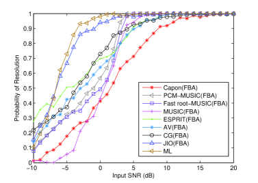
Figure 3: Probability of resolution versus input SNR with $\alpha=0998$, $M=40$, $N=10$, $q=2$, $\tau=0.9$, $r_{\rm opt}=4$.

Before further experiments, we evaluate the performance of the proposed JIO and JIO-RLS algorithms, which is shown in Fig. 4. In this experiment, we set the sources to be uncorrelated but increase the number of sources by setting $q=10$. The number of snapshots is $N=20$ and the array size is $M=40$. From Fig. 4, we find that the proposed JIO and JIO-RLS algorithms show nearly the same probability of resolution with respect to different input SNR values. The same behavior is observed for correlated sources with the use of the FBA technique. These results show that the proposed JIO-RLS algorithm is an efficient alternative to implement the JIO method. In what follows, we will focus on the JIO-RLS algorithm and its comparison to other techniques.

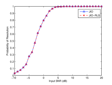
Figure 4: Probability of resolution versus input SNR with $M=40$, $N=20$, $q=10$, $\alpha=0.998$, $\delta=\bar{\delta}=1\times 10^{-3}$, $r_{\rm opt}=5$.

In the next two experiments, the scenario is the same as in Fig.4. We evaluate the probability of resolution and the root mean-square error (RMSE) performance of the proposed JIO-RLS algorithm. Note that the RMSE is computed by averaging over the number of sources in the scenario. Furthermore, we employ the polynomial rooting provided in Section III-B to reduce the search length for the JIO-RLS, which further reduces the complexity. In Fig. 5, the curves between the proposed and ESPRIT algorithms intersect when the input SNR values increase. The proposed algorithm exhibits its ability to work with low SNR values. ESPRIT uses the eigen-decomposition for estimating the signal subspace. ESPRIT with the API approach (ESPRIT(API)) performs direction finding with a low-complexity implementation. However, this performance is poor with a small number of snapshots and thus results in a low probability of resolution, so does MUSIC(API). The AV and CG algorithms also show a low performance when many sources are present in the system.

Fig. 6 presents the RMSE performance for the proposed and existing algorithms under the same scenario as Fig. 5 and compare them with the Cramér-Rao bound (CRB). The RMSE of the proposed JIO-RLS algorithm always keeps a lower level than those of other existing algorithms with different input SNR values. Its values are around $10$ dB higher than the CRB in the threshold region and then approach the CRB curve with the increase of the SNR. The eigen-decomposition algorithms (MUSIC and ESPRIT) are superior to the AV and CG algorithms in this example.

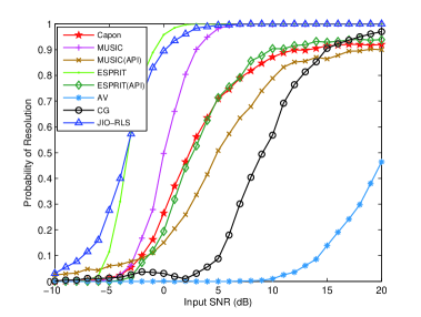
Figure 5: Probability of resolution versus input SNR with $M=40$, $N=20$, $q=10$, $\alpha=1$, $\delta=\bar{\delta}=1\times 10^{-3}$, $r_{\rm opt}=5$.

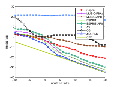
Figure 6: RMSE versus input SNR with $M=40$, $N=20$, $q=10$, $\alpha=1$, $\delta=\bar{\delta}=1\times 10^{-3}$, $r_{\rm opt}=5$.

Fig. 7 and Fig. 8 examine the performance of the proposed and existing algorithms with the FBA technique in a severe scenario, where many sources ($q=10$) are present in the system and the number of snapshots is low ($N=10$). Two sources are highly correlated as explained in the beginning of this section. The number of sensor elements in the array is $M=40$. From Fig. 7, the AV with the FBA technique fails to resolve the DOA at most input SNR values. The CG(FBA) algorithm provides a good resolution but is unstable with respect to different SNR values. The Capon’s, MUSIC, ESPRIT, and the proposed algorithms exhibit relatively high resolutions at high SNR values. The proposed JIO-RLS(FBA) algorithm works well even with very low SNR values. Fig. 8 reflects the RMSE performance of the studied algorithms under the same condition. The proposed JIO algorithm approaches the CRB asymptotically and follows the trend of the CRB as the SNR value increases to $5$ dB.

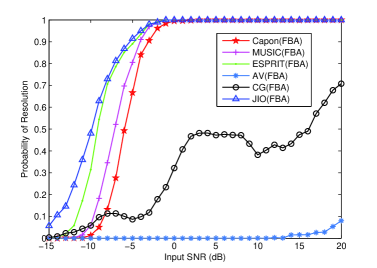
Figure 7: Probability of resolution versus input SNR with $M=40$, $N=10$, $q=10$, $\alpha=1$, $\tau=0.9$, $\delta=\bar{\delta}=1\times 10^{-3}$, $r_{\rm opt}=5$.

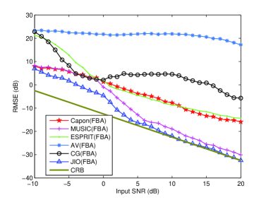
Figure 8: RMSE versus input SNR with $M=40$, $N=10$, $q=10$, $\alpha=1$, $\tau=0.9$, $\delta=\bar{\delta}=1\times 10^{-3}$, $r_{\rm opt}=5$.

In the following results, we consider a situation where the receiver antenna does not know exactly the information of the number of sources $q$. This is more practical since the exact $q$ has to be determined by procedures with extra computational cost and time or by resorting noise threshold with subspace tracking algorithms [28]. The purpose is assess the robustness of the methods in the presence of errors in the model order by measuring the performance degradation of such techniques. The scenario is the same as in Fig. 5. We set the input SNR to $0$ dB and examine the probability of resolution of the proposed and existing algorithms with respect to different values of $q_{w}$. From Fig. 9, the proposed and existing algorithms are evaluated with a variable $q_{w}$ The results show that the proposed JIO and Capon’s algorithms are not significantly affected by different values of $q_{w}$, whereas the performance of the other studied algorithms is significantly degraded for $q_{w}\neq q$. Note that, in this scenario, the number of snapshots $N=20$ is quite small as compared to the number of sensors $M=40$, and this is not sufficient for the existing subspace-based algorithms to construct the signal subspace.

In Fig. 10 and Fig. 11, we set an incorrect number of sources $q_{\textrm{w}}=9$ for the receiver and show the performance versus different input SNR values. Fig. 10 exhibits the probability of resolution for the proposed and existing algorithms. The eigen-decomposition and their related API algorithms fail to solve the DOA estimation problem at all input SNR values since $q$ is critical to the estimation of the signal and noise subspaces. Also, the design of the AV basis and CG residual vectors depends strongly on $q$ and cannot achieve a good direction finding. Capon’s method works well under this condition since it is insensitive to the number of sources. The same result holds for the proposed JIO-RLS algorithm, which outperforms Capon’s method since the joint optimization between the rank reduction matrix and the auxiliary reduced-rank parameter vector leads to an improved performance for the proposed scheme. We also provide the RMSE performance in Fig. 11. The subspace-based algorithms always keep a high RMSE level (above $0$ dB) and do not approach the CRB. The proposed algorithm is not significantly influenced by $q_{\textrm{w}}$ and retains the same trend as the CRB, as depicted in Fig. 5. We also consider the algorithms with the FBA technique in this condition and obtain a comparable result.

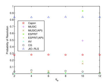
Figure 9: Probability of resolution versus $q_{w}$ with $M=40$, $N=20$, SNR$=0$ dB, $q=10$, $\alpha=0.998$, $\delta=\bar{\delta}=1\times 10^{-3}$, $r_{\rm opt}=5$.

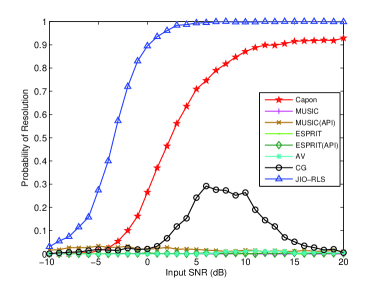
Figure 10: Probability of resolution versus $q_{w}$ with $M=40$, $N=20$, $q=10$, $q_{w}=9$, $\alpha=0.998$, $\delta=\bar{\delta}=1\times 10^{-3}$, $r_{\rm opt}=5$.

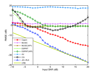
Figure 11: RMSE versus input SNR versus $q_{w}$ with $M=40$, $N=20$, $q=10$, $q_{w}=9$, $\alpha=0.998$, $\delta=\bar{\delta}=1\times 10^{-3}$, $r_{\rm opt}=5$.

VI Concluding Remarks

We have introduced a novel reduced-rank scheme based on the joint iterative optimization of a rank-reduction matrix and an auxiliary parameter vector for DOA estimation. In the proposed scheme, the dimension of the received vector is reduced by the rank-reduction matrix, and the resulting vector is processed by the auxiliary reduced-rank parameter vector for calculating the output power. It provides an iterative exchange of information between the estimated quantities and thus leads to an improved performance. The DOAs of the sources are located by scanning the possible angles and plotting the output power spectrum. The proposed JIO algorithms have been implemented to iteratively estimate the rank-reduction matrix and the auxiliary parameter vector according to the MV design criterion. The polynomial rooting technique has been incorporated in the proposed JIO algorithms to save some computational cost. We have employed the FBA preprocessing to deal with the problem of the highly correlated sources. The proposed algorithms also work well without the exact information of the number of sources. Simulations have shown that the proposed JIO algorithms achieve a superior resolution over the existing algorithms in the scenarios where many sources are present in the system, the array size is large, and the number of snapshots is small.

Derivation of the rank-reduction matrix

Equating (6) to a zero matrix and post multiplying the terms by $\bar{\boldsymbol{g}}_{\theta}$ yields

$$\boldsymbol{T}_{r}\bar{\boldsymbol{g}}_{\theta}=-\lambda_{T_{r}^{\ast}}\boldsymbol{R}^{-1}\boldsymbol{a}(\theta).$$ (24)

Given $\boldsymbol{f}=-\lambda_{T_{r}^{\ast}}\boldsymbol{R}^{-1}\boldsymbol{a}(\theta)$, the matrix $\boldsymbol{T}_{r}$ can be viewed as finding a solution to the linear equation $\boldsymbol{T}_{r}\bar{\boldsymbol{g}}_{\theta}=\boldsymbol{f}$. Assuming $\bar{\boldsymbol{g}}_{\theta}\neq\boldsymbol{0}$, there exist multiple $\boldsymbol{T}_{r}$ satisfying the linear equation in general. Thus, we derive the minimum Frobenius-norm solution for stability. Let us express the quantities involved by

$$\boldsymbol{T}_{r}=[\bar{\boldsymbol{t}}_{1},\bar{\boldsymbol{t}}_{2},\ldots,\bar{\boldsymbol{t}}_{M}]^{H};~{}~{}~{}~{}\boldsymbol{f}=[f_{1},f_{2},\ldots,f_{M}]^{T},$$ (25)

where $\bar{\boldsymbol{t}}_{j}=[\bar{t}_{j,1}^{\ast},\ldots,\bar{t}_{j,r}^{\ast}]^{T}\in\mathbb{C}^{r\times 1}$ with $j=1,\ldots,M$.

The computation of the minimum Frobenius-norm solution transfers to the following $M$ subproblems:

$$\textrm{min}\|\bar{\boldsymbol{t}}_{j}\|^{2},~{}~{}~{}\textrm{subject~{}to~{}}\bar{\boldsymbol{t}}_{j}^{H}\bar{\boldsymbol{g}}_{\theta}=f_{j}.$$ (26)

The solution to (26) is the projection of $\bar{\boldsymbol{t}}_{j}$ onto the hyperplane $\mathcal{H}_{j}=\{\bar{\boldsymbol{t}}_{j}\in\mathbb{C}^{r\times 1}\}:\bar{\boldsymbol{t}}_{j}^{H}\bar{\boldsymbol{g}}_{\theta}=f_{j}$, which is given by

$$\bar{\boldsymbol{t}}_{j}=f_{j}^{\ast}\frac{\bar{\boldsymbol{g}}_{\theta}}{\|\bar{\boldsymbol{g}}_{\theta}\|^{2}}.$$ (27)

Thus, the rank-reduction matrix can be expressed by

$$\boldsymbol{T}_{r}=\boldsymbol{f}\frac{\bar{\boldsymbol{g}}_{\theta}^{H}}{\|\bar{\boldsymbol{g}}_{\theta}\|^{2}}.$$ (28)

Substituting $\boldsymbol{f}=-\lambda_{T_{r}^{\ast}}\boldsymbol{R}^{-1}\boldsymbol{a}(\theta)$ into (28) and following the constraint in (4), we get the $\lambda_{T_{r}^{\ast}}$, which is

$$\lambda_{T_{r}^{\ast}}=-\frac{1}{\boldsymbol{a}^{H}(\theta)\boldsymbol{R}^{-1}\boldsymbol{a}(\theta)}.$$ (29)

From $\boldsymbol{f}$, $\lambda_{T_{r}^{\ast}}$, and $\boldsymbol{T}_{r}$ in (28), we have the expression of the rank-reduction matrix in (7).

Derivation of the Reduced-Rank Vector $\bar{\boldsymbol{g}}_{\theta}$

Equating (8) to zero, we have

$$\bar{\boldsymbol{g}}_{\theta}=\lambda_{\bar{g}_{\theta}^{\ast}}{\bar{\boldsymbol{R}}^{-1}\bar{\boldsymbol{a}}(\theta)},$$ (30)

where $\bar{\boldsymbol{R}}=\mathbb{E}[\bar{\boldsymbol{x}}(i)\bar{\boldsymbol{x}}^{H}(i)]\in\mathbb{C}^{r\times r}$ is the reduced-rank covariance matrix. Substituting (30) into the constraint and equating the terms, we obtain

$$\lambda_{\bar{g}_{\theta}^{\ast}}=(\bar{\boldsymbol{a}}^{H}(\theta)\bar{\boldsymbol{R}}^{-1}\bar{\boldsymbol{a}}(\theta))^{-1},$$ (31)

Substituting $\lambda_{\bar{g}_{\theta}^{\ast}}$ into (30), we obtain

$$\bar{\boldsymbol{g}}_{\theta}=\frac{\bar{\boldsymbol{R}}^{-1}\bar{\boldsymbol{a}}(\theta)}{\bar{\boldsymbol{a}}^{H}(\theta)\bar{\boldsymbol{R}}^{-1}\bar{\boldsymbol{a}}(\theta)},$$ (32)

where $\bar{\boldsymbol{a}}(\theta)=\boldsymbol{T}_{r}^{H}\boldsymbol{a}(\theta)\in\mathbb{C}^{r\times 1}$ is the reduced-rank steering vector with respect to the current scanning angle.

References

- [1]
- [2] H. Krim and M. Viberg, “Two decades of array signal processing research,” IEEE Signal Processing Magazine, vol.13, pp. 67-94, July 1996.
- [3] J. C. Liberti, Jr. and T. S. Rappaport, Smart Antennas for Wireless Communications: IS-95 and Third Generation CDMA Applications, Prentice Hall, 1999.
- [4] H. L. Van Trees, Optimum Array Processing: Part IV of Detection, Estimation, and Modulation Theory, John Wiley & Sons, 2002.
- [5] J. Capon, “High resolution frequency-wavenumber spectral analysis,” IEEE Proc., vol.57, pp.1408-1418, Aug. 1969.
- [6] I. Ziskind and M. Wax, “Maximum likelihood localization of multiple sources by alternating projection,” IEEE Trans. Acoustics, Speech, and Signal Processing, vol. 36, pp. 1553-1560, Oct. 1988.
- [7] R. O. Schmidt, “Multiple emitter location and signal parameter estimation,” IEEE Trans. Antennas and Propagat., vol. 34, pp. 276-280, Mar. 1986.
- [8] R. H. Roy and T. Kailath, “ESPRIT-estimation of signal parameters via rotational invariance techniques,” IEEE Trans. Acoustics, Speech, and Signal Processing, vol. 37, pp. 984-995, Jul. 1989.
- [9] Q. Ren and A. Willis, “Fast root music algorithm,” Electronics Letters, vol. 33, no. 6, pp. 450-451, Mar. 1997.
- [10] A. Morrison and B. S. Sharif, ”High-Resolution Iterative DoA Algorithm for W-CDMA Space-Time Receiver Structures”, IEEE Vehicular Technology Conference - Fall, 2001.
- [11] Y. Chen, P. Honan and U. Tureli, ”Adaptive Reduced-Rank Localization for Multiple Wideband Acoustic Sources”, IEEE Military Communications Conference, 2003.
- [12] R. C. de Lamare and R. Sampaio-Neto, “Blind space-time joint channel and direction of arrival estimation for DS-CDMA systems”, IET Signal Processing, vol. 5, no. 1, pp. 33-39, February 2011.
- [13] R. Grover, D. A. Pados, and M. J. Medley, “Subspace direction finding with an auxiliary-vector basis,” IEEE Trans. on Signal Processing, vol. 55, pp. 758-763, Feb. 2007.
- [14] H. Semira, H. Belkacemi, and S. Marcos, “High-resolution source localization algorithm based on the conjugate gradient,” EURASIP Journal on Adv. in Sig. Proc., vol. 2007, pp. 1-9, Mar. 2007.
- [15] J. Steinwandt, R. C. de Lamare and M. Haardt, “Beamspace direction finding based on the conjugate gradient and the auxiliary vector filtering algorithms”, Signal Processing Volume 93, Issue 4, April 2013, Pages 641-651.
- [16] M. El Korso, R. Boyer, and S. Marcos, “Fast sequential source localization using the projected companion matrix approach,” in Computational Advances in Multi-Sensor Adaptive Processing (CAMSAP), 2009 3rd IEEE International Workshop on, Dec. 2009, pp. 245 -248.
- [17] B. Liao, Z.-G. Zhang and S.-C. Chan, “DOA Estimation and Tracking of ULAs with Mutual Coupling ”, IEEE Transactions on Aerospace and Electronic Systems, vol. 48, no. 1, 2012, pp. 891-905.
- [18] H. Gazzah, “Optimum Antenna Arrays for Isotropic Direction Finding”, IEEE Transactions on Aerospace and Electronic Systems, vol. 47 , no. 2, 2011 , pp. 1482-1489.
- [19] S. D. Blunt, T. Chan and K. Gerlach, “Robust DOA Estimation: The Reiterative Superresolution (RISR) Algorithm”, IEEE Transactions on Aerospace and Electronic Systems, vol. 47 , no. 1, 2011, pp. 332-346.
- [20] R. C. de Lamare and R. Sampaio-Neto, “Reduced-Rank Space-Time Adaptive Interference Suppression With Joint Iterative Least Squares Algorithms for Spread-Spectrum Systems,” IEEE Trans. Veh. Technol., vol.59, no.3, pp.1217-1228, Mar. 2010.
- [21] R. Fa, R. C. de Lamare and L. Wang, “Reduced-rank STAP schemes for airborne radar based on switched joint interpolation, decimation and filtering algorithm”, IEEE Transactions on Signal Processing, vol. 58, no. 8, pp.4182-4194, 2010.
- [22] R. Fa and R. C. de Lamare, ”Reduced-Rank STAP Algorithms using Joint Iterative Optimization of Filters,” IEEE Transactions on Aerospace and Electronic Systems, vol.47, no.3, pp.1668-1684, July 2011.
- [23] R. C. de Lamare and R. Sampaio-Neto, “Reduced-rank adaptive filtering based on joint iterative optimization of adaptive filters,” IEEE Signal Process. lett., vol. 14, no. 12, pp. 980-983, Dec. 2007.
- [24] R. C. de Lamare and R. Sampaio-Neto, “Adaptive Reduced-Rank Processing Based on Joint and Iterative Interpolation, Decimation, and Filtering,” IEEE Transactions on Signal Processing, vol. 57, no. 7, July 2009, pp. 2503 - 2514.
- [25] M. Haardt and A. B. Gershman, “Unitary ESPRIT: how to obtain increased estimation accuracy with a reduced computational burden,” IEEE Trans. Signal Processing, vol. 43, pp. 1232-1242, 1995.
- [26] B. Yang, “Projection approximation subspace tracking,” IEEE Trans. Signal Processing, vol. 44, pp. 95-107, Jan. 1995.
- [27] P. Strobach, “Fast recursive subspace adaptive ESPRIT algorithms,” IEEE Trans. Signal Processing, vol. 46, pp. 2413-2430, Sep. 1998.
- [28] R. Badeau, B. David, and G. Richard, “Fast approximated power iteration subspace tracking,” IEEE Trans. Signal Processing, vol. 53, pp. 2931-2941, Aug. 2005.
- [29] E. E. Tyrtyshnikov, A Brief Introduction to Numerical Analysis, Birkhäuser Boston, 1997.
- [30] L. Wang, R. C. de Lamare, and M. Haardt, “Reduced-rank DOA estimation based on joint iterative subspace recursive optimization and grid search,” IEEE international conference on Acoustics, Speech, and Signal Processing, 2010, pp. 2626-2629, 2010.
- [31] S. Haykin, Adaptive Filter Theory, 4rd ed., Englewood Cliffs, NJ: Prentice-Hall, 1996.
- [32] J. E. Evans, J. R. Johnson, and D. F. Sun, “High resolution angular spectrum estimation techniques for terrain scattering analysis and angle of arrival estimation in ATC navigation and surveillance system,” M.I.T. Lincoln Lab, Lexington, MA, Rep. 582, 1982.
- [33] S. U. Pillai and B. H. Kwon, “Forward/Backword spatial smoothing techniques for coherent signal identification,” IEEE Trans. Acoustics, Speech, and Signal Processing, vol. 37, pp. 8-15, Jan. 1989.
- [34] M. Haardt, Efficient One-, Two-, and Multidimensional High-Resolution Array Signal Processing, Shaker Verlag, Aachen, 1997.
- [35] M. D. Zoltowski, M. Haardt, and C. P. Mathews, “Closed-form 2-D angle estimation with rectangular arrays in element space or beamspace via unitary ESPRIT,” IEEE Trans. Signal Processing, vol. 44, pp. 316-328, Feb. 1996.
- [36] J. A. Gansman, M. D. Zoltowski, and J. V. Krogmeier, “Multidimensional multirate DOA estimation in beamspace,” IEEE Trans. Signal Processing, vol. 44, pp. 2780-2792, Nov. 1996.
- [37] M. D. Zoltowski, G. M. Kautz, and S. D. Silverstein, “Beamspace root-MUSIC,” IEEE Trans. Signal Processing, vol. 41, pp. 344-364, Jan. 1993.
- [38] A. B. Gershman, “Direction finding using beamspace root estimator banks,” IEEE Trans. Signal Processing, vol. 46, Nov. 1998.
- [39] T. J. Shan, M. Max, and T. Kailath, “On spatial smoothing for estimation of coherent signals,” IEEE Trans. on Acoustics, Speech, and Signal Processing, vol. ASSP-33, pp. 802-811, Aug. 1985.
- [40] G. H. Golub and C. F. Van Loan, Matrix Comuputations, 3rd ed. Baltimore, MD: Johns Hopkins Univ. Press, 1996.
- [41] P. Stoica and A. B. Gershman, “Maximum-likelihood DOA estimation by data-supported grid search,” IEEE Signal Processing Letters., vol. 6, pp. 273-275, Oct. 1999.