A directional wave measurement attack against the Kish key distribution system

Abstract

The Kish key distribution system has been proposed as a classical alternative to quantum key distribution. The idealized Kish scheme elegantly promises secure key distribution by exploiting thermal noise in a transmission line. However, we demonstrate that it is vulnerable to nonidealities in its components, such as the finite resistance of the transmission line connecting its endpoints. We introduce a novel attack against this nonideality using directional wave measurements, and experimentally demonstrate its efficacy. Our attack is based on causality: in a spatially distributed system, propagation is needed for thermodynamic equilibration, and that leaks information.

The Kish key distribution (KKD) system, based on Kirchhoff’s laws and Johnson noise (KLJN) Kish (2006a) has been proposed as a classical alternative to quantum key distribution (QKD) Bennett and Brassard (1984). Eschewing expensive and environmentally-sensitive optics, it can be implemented economically in a wider variety of systems than QKD.

Figure 1: We determine the forward- and reverse-travelling waves in this idealized KKD system. Practical systems would include low-pass filters and instrumentation that do not affect the steady-state signal. The mean-squared voltages $\langle V_{a}^{2}(t)\rangle$ and $\langle V_{b}^{2}(t)\rangle$ are proportional to the resistances $R_{a}$ and $R_{b}$ respectively. We perform our analysis in terms of the reflection coefficients $\Gamma_{A}$ and $\Gamma_{B}$.

The KKD system is claimed Kish (2006a) to derive unconditional security from the second law of thermodynamics—the idea being that net power cannot flow from one resistor to the other under equilibrium.

An idealised KKD system is shown in Figure 1. Alice and Bob each apply a noise signal to a line through a series resistor. The voltage on the line is unchanged if the terminals of Alice and Bob are swapped; if the mean-square voltages applied by Alice and Bob are proportional to $R_{a}$ and $R_{b}$ respectively then no average power flows through the line, and in the ideal case an eavesdropper, Eve, cannot determine which end has which resistance Kish (2006a); Gingl and Mingesz (2014). If Alice and Bob randomly choose their resistances—resulting in corresponding noise amplitudes—to be either $R_{h}$ or $R_{l}$, three possibilities avail themselves: both choose $R_{h}$, both choose $R_{l}$, or one chooses $R_{h}$ and the other chooses $R_{l}$. In this third case, Alice knows the value of her own resistor, and so can deduce Bob’s resistor via noise spectral analysis, and vice-versa. However, an eavesdropper lacks this knowledge, and so in the ideal case Alice and Bob have secretly shared one bit of information.

It has been claimed Kish and Horvath (2009) that transmission line theory does not apply to the the KKD system when operated at frequencies below $f_{c}=\nu/({2L})$, where $L$ is the transmission line length and $\nu$ the signal propagation velocity, because wave modes do not propagate below this cutoff. We demonstrate that this is not the case by constructing a directional wave measurement device that is then used for a successful finite-resistance attack against the system. The position that frequencies below $f_{c}$ do actually propagate is also supported by the fact that, at low frequencies, a coaxial cable is known to only support TEM modes—these modes are known to have no low frequency cutoff (Jackson, 1999, p. 358). An exception occurs when the two ends of the line are held at equal potential; only standing waves possessing a frequency that is an integer multiple of ${\nu}/({2L})$ can fulfill these boundary conditions (Griffiths, 2005, p. 31). However, the the KKD system differs in allowing arbitrary potentials to appear at the ends of the line, and so does not support standing waves at the frequency of operation.

Several attacks against the KKD system exist, however none thus far have been shown experimentally to substantially reduce the security of the system Mingesz et al. (2008).

The first attacks, proposed by Scheuer and Yariv Scheuer and Yariv (2006), rely upon imperfections in the line connecting the two terminals; the first exploits transients generated by the resistor-switching operation, while the second exploits the line’s finite resistance. The former is foiled by the addition of low-pass filters to the terminals Kish (2006b), while the latter was shown to leak less than $1\text{\,}\mathrm{\char 37\relax}$ of bits Kish (2006b); Mingesz et al. (2008) in a practical system.

An attack by Hao Hao (2006); Kish (2006c) instead focuses upon imperfections of the terminals; inaccuracies in the noise temperatures of Alice and Bob create an information leak. However, it was demonstrated Kish (2006c); Mingesz et al. (2008) that noise can be digitally generated with a sufficiently accurate effective noise temperature to prevent this attack from being useful in practice.

A theoretical argument has been made by Bennett and Riedel Bennett and Riedel (2013) that no purely classical electromagnetic system can be unconditionally secure due to the structure of Maxwell’s equations. It is argued that the upper bound on secrecy rate by Maurer Maurer (1993) must be zero because of the locally-causal nature of classical electromagnetics, and so an eavesdropper can perfectly reconstruct the key with the aid of a directional coupler. Kish, et al. Kish et al. (2013) responded that a nonzero secrecy rate is unnecessary in practice, provided it can be achieved in the ideal limit.

We begin our attack by analyzing the system in Figure 1 to determine the forward- and reverse-travelling waves through the transmission line. Let us denote the equivalent noise voltages of Alice and Bob $V_{a}(t)$ and $V_{b}(t)$ respectively, and the waves injected onto the line $V^{\prime}_{a}(t)$ and $V^{\prime}_{b}(t)$. These are related by

$$V^{\prime}_{a}(t) =\frac{1}{2}(1-\Gamma_{A})V_{a}(t)$$ (1)

$$V^{\prime}_{b}(t) =\frac{1}{2}(1-\Gamma_{B})V_{b}(t).$$ (2)

Noting that the mean-squared thermal noise voltage is $\langle V^{2}\rangle=4kTBR$, we find that

$$\left\langle{V^{\prime}_{a}}^{2}\right\rangle =kTBZ_{0}(1-\Gamma_{A}^{2})$$ (3)

$$\left\langle{V^{\prime}_{b}}^{2}\right\rangle =kTBZ_{0}(1-\Gamma_{B}^{2}).$$ (4)

As the transmission line in the KKD system is short—and so the forward- and reverse-travelling waves are equal throughout the line except for a loss factor $\alpha$—we may write the left- and right-travelling waves at Bob’s and Alice’s ends of the line respectively as

$$V_{+}(t) =V^{\prime}_{a}(t)+\alpha\Gamma_{A}V_{-}(t)$$ (5)

$$V_{-}(t) =V^{\prime}_{b}(t)+\alpha\Gamma_{B}V_{+}(t)$$ (6)

and so

$$V_{+}(t) =\frac{V^{\prime}_{a}(t)+\alpha\Gamma_{A}V^{\prime}_{b}(t)}{1-\alpha^{2}\Gamma_{A}\Gamma_{B}}$$ (7)

$$V_{-}(t) =\frac{V^{\prime}_{b}(t)+\alpha\Gamma_{B}V^{\prime}_{a}(t)}{1-\alpha^{2}\Gamma_{A}\Gamma_{B}}.$$ (8)

We may write this in matrix form ${\bf v}_{d}(t)=A{\bf v}_{i}(t)$ and so find the covariance matrix $\mathcal{C}=A\mathcal{C}_{i}A^{t}$ of the directional components:

$$\mathcal{C} =\frac{kTBZ_{0}}{\left(1-\alpha^{2}\Gamma_{A}\Gamma_{B}\right)^{2}}\left[\begin{matrix}1-\alpha^{2}\Gamma_{A}^{2}\Gamma_{B}^{2}+(\alpha^{2}-1)\Gamma_{A}^{2}&\alpha\Gamma_{A}(1-\Gamma_{B}^{2})+\alpha\Gamma_{B}(1-\Gamma_{A}^{2})\\ \alpha\Gamma_{A}(1-\Gamma_{B}^{2})+\alpha\Gamma_{B}(1-\Gamma_{A}^{2})&1-\alpha^{2}\Gamma_{A}^{2}\Gamma_{B}^{2}+(\alpha^{2}-1)\Gamma_{B}^{2}\end{matrix}\right].$$ (9)

When the line is lossless and so $\alpha=1$, Eqn. 9 is invariant under permutation of $\Gamma_{A}$ and $\Gamma_{B}$, and so the covariance matrix provides no information on the choice of resistors. However, when $\alpha<1$ this property fails to hold, allowing the choices of $\Gamma_{A}$ and $\Gamma_{B}$ to be determined from the distribution of $(v_{+},v_{-})$.

A directional coupler separates forward- and reverse-travelling waves on a transmission line Pozar (1998). We have constructed a similar device using differential measurements across a delay line, shown in Figure 2.

Consider the d’Alembert solution (Jackson, 1999, Eqn. 7.7) to the wave equation in a medium with propagation velocity $\nu$,

$$v(t,x) =v_{+}\left(t-\frac{x}{\nu}\right)+v_{-}\left(t+\frac{x}{\nu}\right).$$ (10)

The forward-travelling component $v_{+}(\tau)$ differs from the reverse-travelling component $v_{-}(\tau)$ in the sign of its spatial argument. We use this to our advantage by computing the linear combinations

$$\frac{\partial v}{\partial t}-\nu\frac{\partial v}{\partial x} =2\frac{dv_{+}}{dt}$$ (11)

$$\frac{\partial v}{\partial t}+\nu\frac{\partial v}{\partial x} =2\frac{dv_{-}}{dt},$$ (12)

yielding the forward- and reverse-travelling waves as we desire. All that remains, then, is to determine $\partial v/\partial t$ and $\partial v/\partial x$.

The time derivative $\partial v/\partial t$ may be determined digitally from sampled values of $v(t)$. The spatial derivative is approximated as being proportional to the voltage across a short delay line, shown in Figure 2.

Figure 2: The analog frontend of the directional wave measurement device. Buffering, offset, gain control, and clamping are not shown. An instrumentation amplifier is used to measure the voltage across a $1.5\text{\,}\mathrm{m}$ length of coaxial cable, providing an estimate of $\partial v/\partial x$. After offset and gain adjustments, the signals are simultaneously sampled by the 12-bit ADCs of an STM32F407 microcontroller.

After digitisation, we high-pass filter the signals $V$ and $V_{x}$ in order to remove any DC offsets or mains interference. The signals are then combined to produce the left- and right-travelling waves. The time-derivative $\partial v/\partial t$ can be approximated by a difference operator, however in order to accommodate for the unknown propagation velocity and delay line length, common-mode leakage into $V_{x}$, and losses in the delay line, we instead use a first-order least-mean-squares (LMS) adaptive filter Haykin (2002) for initial calibration. A signal source is applied to one port and the other is terminated; this produces a right-travelling wave on the line, but none travelling to the left. The left-travelling output $V_{-}$ is used as an error signal for the LMS filter, suppressing any contribution from the right-travelling wave.

Figure 3: The digital signal processing of the directional wave measurement device, implemented on an STM32F407 microcontroller. Offset removal is not shown. A least-mean-squares filter is used at startup to determine the necessary filter coefficients; a signal is applied to one port while the other is connected to a terminator, and the filter coefficients adjusted to force $V_{-}=0$. Filter updates are disabled once the apparent reflection coefficient becomes sufficiently small.

The real part of the reflection coefficient, seen looking out of the right port, is computed by a cross-correlation between left- and right-travelling waves. When this falls below $0.01$, calibration is declared complete and filter updates cease. After calibration, we validate the system by configuring it as a reflectometer. Open and shorted measurements are made, yielding reflection coefficients of $+1$ and $-1$ respectively. The reflection coefficients of several resistors are also measured, again yielding the expected values.

We have described the implementation of a directional wave measurement device using differential measurements across a delay line. While we might measure the power travelling in each direction in order to determine the resistor configuration, the distributions to be distinguished are very similar, resulting in a relatively large bit-error rate (BER) as was shown in Kish (2006b). However, comparison of the variances of $v_{+}$ and $v_{-}$ is suboptimal. We derive an improved test using Bayesian methods and demonstrate that the two cases can be far more easily distinguished.

Knowing the covariance matrices of $v_{+}(t)$ and $v_{-}(t)$ for each hypothesis, we may use Bayes’ theorem Larsen and Marx (2012) to determine the probability of each configuration. Let $C=0$ and $C=1$ refer to the events that $(R_{a},R_{b})=(R_{h},R_{l})$ and vice-versa, respectively. Then,

$$P[C=0|{\bf v_{+}}\cap{\bf v_{-}}] =\frac{P[{\bf v_{+}}\cap{\bf v_{-}}|C=0]P[C=0]}{P[{\bf v_{+}}\cap{\bf v_{-}}]}$$ (13)

$$=\frac{\frac{1}{2}p_{0}({\bf v_{+}},{\bf v_{-}})}{\frac{1}{2}p_{0}({\bf v_{+}},{\bf v_{-}})+\frac{1}{2}p_{1}({\bf v_{+}},{\bf v_{-}})}$$ (14)

$$=\frac{1}{1+\frac{p_{1}({\bf v_{+}},{\bf v_{-}})}{p_{0}({\bf v_{+}},{\bf v_{-}})}},$$ (15)

where $p_{0}(\cdot,\cdot)$ and $p_{1}(\cdot,\cdot)$ are the multivariate Gaussian PDFs for the measurements from each respective configuration.

The most probable state, then, is given by the maximum-likelihood estimator Larsen and Marx (2012)

$$\hat{C}=\begin{cases}0&\text{if }p_{0}({\bf v_{+}},{\bf v_{-}})>p_{1}({\bf v_{+}},{\bf v_{-}})\\ 1&\text{if }p_{0}({\bf v_{+}},{\bf v_{-}})<p_{1}({\bf v_{+}},{\bf v_{-}}).\\ \end{cases}$$ (16)

The comparison is more conveniently made in terms of the log-likelihood, which for the $n$-variate zero-mean Gaussian distribution with covariance matrix $\Sigma$ is given by (Cover and Thomas, 2006, p. 250)

$$\log p_{\Sigma}({\bf x}) =\log\left[\frac{1}{\left(2\pi\right)^{\frac{n}{2}}\left|K\right|^{\frac{1}{2}}}e^{-\frac{1}{2}{\bf x}^{T}\Sigma^{-1}{\bf x}}\right]$$ (17)

$$=-\frac{1}{2}\log\left|\Sigma\right|-\frac{n}{2}\log\left(2\pi\right)-\frac{1}{2}{\bf x}^{T}\Sigma^{-1}{\bf x}.$$ (18)

Noting that $$\Sigma \Sigma=KK^{T}$$ is positive-definite, we may write it in terms of its Cholesky decomposition , and so

$$=-\frac{1}{2}\log\left|\Sigma\right|-\frac{n}{2}\log\left(2\pi\right)-\frac{1}{2}\left\|K^{-1}{\bf x}\right\|^{2}.$$ (19)

Only the final term depends upon the data, and there only through the total power of a group of signals $K^{-1}{\bf x}$ formed by linear combinations of the measured waves.

It should be noted that this estimator differs substantially from that proposed in Scheuer and Yariv (2006), which makes a simple comparison of variances. The measured variables in our case are collected simultaneously and so exhibit the heavy correlations of Eqn. 9. With these correlations, the likelihood-ratio test provides far better performance than the difference in the variances of the marginal distributions would suggest. However, if the voltage and current measurements are considered separately, as in Kish (2006b); Mingesz et al. (2008) where only the marginal distributions of each measurement are computed, these correlations vanish and so the estimator described in Eqns. 16 and 19 has substantially less power. The distribution of test statistics is shown in Figure 4 for a loss of $0.1\text{\,}\mathrm{dB}$. The presence of correlation causes the distributions of test statistics to differ substantially, where otherwise they would be almost indistinguishable.

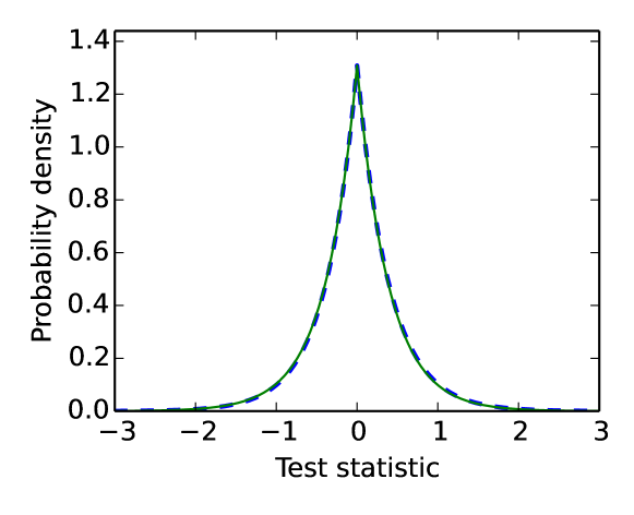
(a) Uncorrelated measurements

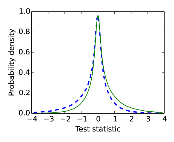
(b) Correlated measurements

Figure 4: Log likelihood-ratio test statistics for each permutation of resistors in Eqn. 9, as in Eqn. 19 with scaling-factors omitted. The dashed lines correspond to the case where $(R_{a},R_{b})=(R_{l},R_{h})$, and the solid lines to $(R_{a},R_{b})=(R_{h},R_{l})$. Parameters are $R_{l}=$1\text{\,}\mathrm{k\SIUnitSymbolOhm}$,R_{h}=$10\text{\,}\mathrm{k\SIUnitSymbolOhm}$,Z_{0}=$50\text{\,}\mathrm{\SIUnitSymbolOhm}$$, and $\alpha=$-0.1\text{\,}\mathrm{dB}$$. In Figure 4a the covariances are set to zero, and so Eqn. 16 reduces to a simple power comparison. The distributions are almost indistinguishable. In Figure 4b, the measurement variables are drawn from a correlated bivariate distribution having the same marginal variances, and are far more distinguishable. In either case, as losses increase and so the variances of the measurements and transformed measurements respectively differ more greatly, the two distributions, which mirror each other about zero, become increasingly assymmetric and so far more distinguishable.

The results of simulation for various values of loss are shown in Figure 5. A pair of white noise processes are generated, Fourier-transformed, and the undesirable frequency components removed. They are combined according to Eqn. 8 to produce the voltage waves, and the maximum-likelihood estimator is used to determine the resistor configurations. This demonstrates that our estimator can differentiate the two distributions without the unreasonably large sample sizes that were previously thought necessary Kish (2006b).

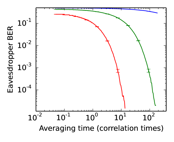
Figure 5: Simulated eavesdropper bit-error-rate as a function of averaging time, for line attenuations of 0.01, 0.1, and 1.0 decibels respectively from top to bottom. The link parameters are $R_{L}=$1\text{\,}\mathrm{k\SIUnitSymbolOhm}$,R_{H}=$1\text{\,}\mathrm{k\SIUnitSymbolOhm}$,Z_{0}=$50\text{\,}\mathrm{\SIUnitSymbolOhm}$$. Note that the averaging time is expressed in multiples of $200\text{\,}\mathrm{\SIUnitSymbolMicro s}$. This is the correlation time (i.e. reciprocal of the system bandwidth) so that the results are bandwidth independent. Transmission lines with greater loss are more susceptible to attack, with substantial attenuations providing little protection. The error rates are estimated from a sample size of $10^{5}$, with $2\sigma$ error bars shown.

Having demonstrated our attack in simulation, we proceed to experimental validation of the model. The estimation of $\partial v/\partial x$ is key to the operation of the device, however the synthesis provided above is dependent upon a wave-based analysis of the system. We therefore measure experimentally the frequency response of the electronically-estimated $\partial v/\partial x$, shown in Figure 6, with a wave travelling in a single direction in order to verify that our analysis is appropriate.

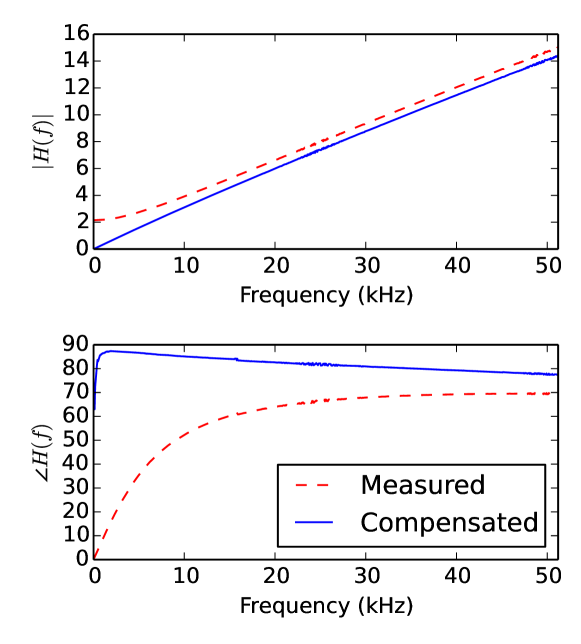
Figure 6: Measured frequency response of the $\partial v/\partial x$ estimation circuit in Figure 2. The derivative increases linearly with frequency, as would be expected from the d’Alembert solution to the wave equation. The response $H(0)$ at DC is subtracted in order to remove the effect of wire resistance, yielding the ‘compensated’ curves above. After this correction we see $\angle H(f)$ approximating the expected $+90^{\circ}$ constant phase response, slightly drooping due to the limited frequency response of the system.

We expect to see a magnitude response linear in frequency and a constant $+90^{\circ}$ phase response. This agrees with the experimental results shown in Figure 6, validating our analysis, and demonstrates that the signal through a short transmission line indeed propagates as a wave, in contradiction to the theoretical claims of Kish and Horvath (2009).

We have implemented the attack described above, using resistances $R_{l}=$1\text{\,}\mathrm{k\SIUnitSymbolOhm}$$, $R_{h}=$10\text{\,}\mathrm{k\SIUnitSymbolOhm}$$, and a coaxial transmission line of characteristic impedance $Z_{0}=$50\text{\,}\mathrm{\SIUnitSymbolOhm}$$. The voltage sources are produced by an arbitrary waveform generator, producing independent normally-distributed voltages over a frequency range of $500\text{\,}\mathrm{Hz}$–$5500\text{\,}\mathrm{Hz}$. The bandwidth $B=$5\text{\,}\mathrm{kHz}$$ results in an approximate correlation time of $B^{-1}=$200\text{\,}\mathrm{\SIUnitSymbolMicro s}$$ Kish (2006d). Each configuration is set and the covariance matrices from Eqn. 9 are measured during the setup phase. Resistor configurations are randomly selected as would be the case in an operational system, and the log-likelihood ratios are computed for the measured values of $v_{+}$ and $v_{-}$. Their differences are thresholded to compute (16), providing the bit-error rates in Figure 7. Even modest losses allowed almost all bits to be determined correctly, showing that the technique simulated in Figure 5 can be applied in practice.

By applying a threshold to the likelihood ratios, we may estimate the agreed bits and so determine the error rate of Eve. We see that even with the minuscule losses of the test system, Eve can acquire a substantial proportion of the agreed bits.

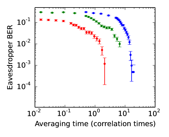
Figure 7: Measured eavesdropper bit-error-rate as a function of averaging time and line attenuation. The line is approximately $2\text{\,}\mathrm{m}$ in length and has a loss of less than $0.1\text{\,}\mathrm{dB}$. From top to bottom, $0\text{\,}\mathrm{dB}$, $0.1\text{\,}\mathrm{dB}$, and $1\text{\,}\mathrm{dB}$ of additional attenuation provided by inserting an in-line attenuator at one end of the line.

The technique above exploits imperfections in the KKD implementation; while it might be theoretically possible to counter this attack by reduction of losses as proposed in Kish (2006b), the reduction of losses substantially below $0.1\text{\,}\mathrm{dB}$ ensures that this will be infeasible for all but the shortest or slowest of links.

This raises the question of why our attack should succeed where existing finite-resistance attacks have failed. The attack of Scheuer and Yariv Scheuer and Yariv (2006) considered only the variances of the measured variables. Our attack exploits the large correlation between waves in each direction; the estimator used above partially removes this common signal, increasing the ability to distinguish between the two cases statistically.

We have demonstrated an attack against the KKD key distribution system that exploits losses within the connecting transmission line. The attack has been shown experimentally to correctly determine more than $99.9\text{\,}\mathrm{\char 37\relax}$ of bits transmitted over a $2\text{\,}\mathrm{m}$ transmission line within 20 correlation times. As this attack requires that losses be reduced to a fraction of a decibel in order to maintain a meaningful level of security, modifications to the system will be necessary in order to produce a secure link of any significant length and bitrate.

References

- Kish (2006a) L. B. Kish, Physics Letters A 352, 178 (2006a).
- Bennett and Brassard (1984) C. H. Bennett and G. Brassard, in Proc. IEEE Int. Conf. Computers, Systems, and Signal Processing (Bangalore, India, 1984) pp. 175–179.
- Gingl and Mingesz (2014) Z. Gingl and R. Mingesz, PLoS ONE 9, e96109 (2014).
- Kish and Horvath (2009) L. B. Kish and T. Horvath, Physics Letters A 373, 2858 (2009).
- Jackson (1999) J. D. Jackson, Classical Electrodynamics, 3rd ed. (Wiley, 1999).
- Griffiths (2005) D. J. Griffiths, Introduction to Quantum Mechanics, 2nd ed. (Prentice Hall, 2005).
- Mingesz et al. (2008) R. Mingesz, Z. Gingl, and L. B. Kish, Physics Letters A 372, 978 (2008).
- Scheuer and Yariv (2006) J. Scheuer and A. Yariv, Physics Letters A 359, 737 (2006).
- Kish (2006b) L. B. Kish, Physics Letters A 359, 741 (2006b).
- Hao (2006) F. Hao, IEE Proceedings—Information Security 153, 141 (2006).
- Kish (2006c) L. B. Kish, Fluctuation and Noise Letters 6, C37 (2006c).
- Bennett and Riedel (2013) C. H. Bennett and C. J. Riedel, arXiv:1303.7435v1 [quant-ph] (2013).
- Maurer (1993) U. M. Maurer, IEEE Transactions on Information Theory 39, 733 (1993).
- Kish et al. (2013) L. B. Kish, D. Abbott, and C. G. Granqvist, PLOSONE 8, e81810 (2013).
- Pozar (1998) D. M. Pozar, Microwave Engineering (Wiley, 1998).
- Haykin (2002) S. Haykin, Adaptive Filter Theory, 4th ed. (Prentice Hall, 2002).
- Larsen and Marx (2012) R. J. Larsen and M. L. Marx, An Introduction to Mathematical Statistics and Its Applications (Pearson, 2012).
- Cover and Thomas (2006) T. M. Cover and J. A. Thomas, Elements of Information Theory, 2nd ed. (Wiley, 2006).
- Kish (2006d) L. B. Kish, Fluctuation and Noise Letters 6, L57 (2006d).