A meshless method for compressible flows with the HLLC Riemann solver

Abstract

The HLLC Riemann solver, which resolves both the shock waves and contact discontinuities, is popular to the computational fluid dynamics community studying compressible flow problems with mesh methods. Although it was reported to be used in meshless methods, the crucial information and procedure to realise this scheme within the framework of meshless methods were not clarified fully. Moreover, the capability of the meshless HLLC solver to deal with compressible liquid flows is not completely clear yet as very few related studies have been reported. Therefore, a comprehensive investigation of a dimensional non-split HLLC Riemann solver for the least-square meshless method is carried out in this study. The stiffened gas equation of state is adopted to capacitate the proposed method to deal with single-phase gases and/or liquids effectively, whilst direct applying the perfect gas equation of state for compressible liquid flows might encounter great difficulties in correlating the state variables. The spatial derivatives of the Euler equations are computed by a least-square approximation and the flux terms are calculated by the HLLC scheme in a dimensional non-split pattern. Simulations of gas and liquid shock tubes, moving shock passing a cylinder, internal supersonic flows in channels and external transonic flows over aerofoils are accomplished. The current approach is verified by extensive comparisons of the produced numerical outcomes with various available data such as the exact solutions, finite volume mesh method results, experimental measurements or other reference results.

1 Introduction

For compressible flow problems in computational fluid dynamics (CFD), the physical features such as shock waves and/or contact discontinuities, across which the fluid density, velocity and/or pressure vary abruptly, often appear in the solution. They are usually referred as Riemann problems (named after Bernhard Riemann) in mathematics [1]. Based on the characteristics analysis, the exact solutions can be obtained through iterations and they perform well for simple problems [2, 3]. However, exact Riemann solvers are computational expensive for two- and three-dimensional problems, for which thousands or millions of mesh elements are used to discretise the whole flow domain [4]. Therefore, great efforts have been made in the past several decades to develop the efficient approximate Riemann solvers.

For this purpose, Harten, Lax and van Leer proposed the HLL Riemann solver with a two-wave model resolving three constant states [5]. To restore the intermediate wave missing from the HLL solver, Toro et al. [6, 7] proposed the HLLC Riemann solver composing a three-wave model to separate four averaged states. Consequently the contact discontinuity was identified by the HLLC solver [6]. Batten et al. further modified the wavespeeds estimate of the scheme, assuming the intermediate wave speed equals to the average normal velocity between the intermediate left and right acoustic waves [8, 9]. The HLLC scheme is a versatile approximate Riemann solver and it has attractive features including exact resolution of isolated contact and shock waves, positivity preservation and enforcement of entropy condition [8, 10]. It is now one of the most popular approximate Riemann solvers used by the researchers investigating compressible flow problems with mesh methods [1, 9, 11, 12, 13, 10, 14]. These facts trigger off our intention to extend the HLLC scheme from mesh methods to meshless methods.

Meshless methods are relatively new and currently they are not as mature as mesh based methods including finite difference, finite element and finite volume. Since the important work of Batina in meshless methods for computational gas dynamics [15, 16], many studies have been accomplished to explore the advantages of these methods for simulating external aerodynamics problems using the JST (Jameson-Schmidt-Turkey) scheme or upwind schemes [17, 18, 19, 20, 21, 22, 23, 24, 25, 26, 27, 28, 29]. Some concerns were raised by researchers regarding the efficiency of meshless methods, because these kinds of methods are usually not faster or even slower than mesh methods on a per-point basis as indicated by Batina[16]. While this topic is beyond the scope of the current work, readers may refer to the following important works using implicit method [22, 17, 26], adaptive method [27, 21], hybrid method [19, 38] and multi-level cloud method [18], which have been accomplished to address this issue. It was noticed by the current authors that the HLLC scheme was claimed to be used in meshless methods for gas dynamics problems [32]. Unfortunately, it was not clearly stated whether the flux terms were computed in a dimensional split or non-split manner, and the wavespeeds estimate for the HLLC scheme was not clarified. After a relatively thorough investigation of the above-mentioned works for meshless methods, it is interesting to discover that these researcheres mainly focused on the compressible gas flows and only the perfect gas equation of state (PG-EOS) was adopted to correlate the state variables (density, pressure and temperature/energy). Consequently, it is a little difficult to foresee whether they will extend the meshless methods to the simulation of compressible liquids for high pressure and/or high speed flow problems in hydrodynamics.

The objective of the present work is to conduct a comprehensive study of the HLLC approximate Riemann solver within the framework of least-square meshless method (LSMM) for compressible flows. A dimensional non-split meshless HLLC Riemann solver is presented with specific implementation details in this paper. A corresponding step-by-step instructive computing algorithm, which is easy to follow, is also provided in the paper. The main work concentrates on the compressible gas flows, which are very important for computational aerodynamics. Referring the liquid flows in hydrodynamics, they are generally considered to be incompressible due to their small density variations. However, for high pressure and/or high speed problems, simply assuming the liquids as incompressible will encounter difficulties in numerical simulations [46, 47, 48, 41, 49, 50, 51]. Therefore, a tentative study of the compressible liquid flow problems with the meshless HLLC solver is also presented to gauge the capability of the method. Considering the fact that the PG-EOS may be not very suitable for liquids to correlate the state variables, the stiffened gas equation of state (SG-EOS) is adopted in the present work. This enables the presented method to effectively handle the gases and liquids with the appropriate polytropic constants and pressure constants. To the best of our knowledge, the implementation of the HLLC solver for the SG-EOS in meshless methods has not been reported in the literature.

The rest of this paper is organised as follows. The governing equations indicating the conservation of mass, momentum and energy for compressible flows are presented in Section 2. The basic theory of LSMM is described in Section 3.1, the spatial discretisation of the Euler equations is presented in Section 3.2. The HLLC approximate Riemann solver for LSMM is illustrated in Section 3.3 followed with the time integration method described in Section 3.4. Numerical examples of one-dimensional gas and liquid shock tubes, two-dimensional moving shock passing a cylinder, internal supersonic flows in channels and external transonic flows over aerofoils are given in Section 4 with intensive comparisons to various available reference results. Conclusions are drawn in Section 5.

2 Governing equations

The present work focuses on the two-dimensional single-phase inviscid compressible flows, of which the mathematical model is represented by the Euler equations indicating the conservation of mass, momentum and energy. The differential forms of these equations can be expressed as

$$\frac{\partial\mathbf{U}}{\partial t}+\frac{\partial\mathbf{E}}{\partial x}+\frac{\partial\mathbf{F}}{\partial y}=0$$ (1)

where $\mathbf{U}$ is a vector of conservative variables, $\mathbf{E}$ and $\mathbf{F}$ are the flux terms, and are defined as

$$\mathbf{U}=\begin{bmatrix}\rho\\ \rho u\\ \rho v\\ \rho e_{\rm t}\end{bmatrix},\quad\mathbf{E}=\begin{bmatrix}\rho u\\ \rho u^{2}+p\\ \rho uv\\ (\rho e_{\rm t}+p)u\end{bmatrix},\quad\mathbf{F}=\begin{bmatrix}\rho v\\ \rho uv\\ \rho v^{2}+p\\ (\rho e_{\rm t}+p)v\end{bmatrix}$$ (2)

in which, $\rho$ is the density, $p$ is the pressure, $u$ and $v$ are the components of velocity vector $\vec{V}$ along $x$ and $y$ axes respectively. The total energy per volume $\rho e_{\rm t}$ is the sum of the internal energy $\rho e_{\rm i}$ and kinematic energy $\rho e_{\rm k}$, they are evaluated by the following formulae

$$\rho e_{\rm t}=\rho e_{\rm i}+\rho e_{\rm k}$$ (3a)

$$\rho e_{\rm k}=\frac{1}{2}\rho(u^{2}+v^{2})$$ (3b)

$$\rho e_{\rm i}=e_{\rm i}(\rho,p)$$ (3c)

The stiffened gas equation of state (SG-EOS) is used in the present work, therefore the internal energy is given by

$$\rho e_{\rm i}=\frac{p+\gamma p_{\rm c}}{\gamma-1}$$ (4)

where $p_{\rm c}$ is the pressure constant and $\gamma$ is the polytropic constant. For ideal gas, the pressure constant vanishes ($p_{\rm c}=0$) and the polytropic constant equals to the ratio of specific heats ($\gamma=1.4$ for air). The speed of sound can be calculated by the following formula

$$c^{2}=\frac{\gamma}{\rho}(p+p_{\rm c})$$ (5)

3 Numerical methods

Meshless methods are relatively new for the compressible flow applications compared to the traditional mesh-based methods including finite difference, finite element and finite volume methods. In this section, the basic theory of LSMM is firstly described and the spatial discretisation procedure of the Euler equations is explained. Then a dimensional non-split implementation of the HLLC scheme in LSMM is presented. Finally the temporal discretisation of the governing equations is given.

3.1 Basic theory of LSMM

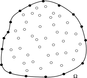
Figure 1: Meshless points distribution in the domain $\Omega$

The essential idea of meshless methods is to introduce a number of scattered points $P_{i}(i=1,2,3,\ldots,N)$ to a domain $\Omega$. The connectivity between the points is not necessary to be considered. Fig. 1 gives an example of the domain discretisation using meshless points. For each point, several points around it are chosen to form a cloud of points [15, 16, 34, 35]. Fig. 2 shows a cloud of points $C_{i}$, in which the point $i$ is named the centre and the other points are called the satellites ($P_{ij}$ is the midpoint between $i$ and $j$).

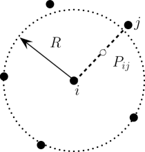
Figure 2: A typical meshless cloud of points

The coordinate difference between the satellite $j$ and the centre $i$ can be expressed as

$$h_{j}^{i}=x_{j}-x_{i},\qquad l_{j}^{i}=y_{j}-y_{i}$$ (6)

For simplicity, $h_{j}$ and $l_{j}$ are used to denote $h_{j}^{i}$ and $l_{j}^{i}$, respectively. The vector ${\mathbf{r}}^{i}_{j}=(h_{j},l_{j})$ starts from $i$ to $j$, its length is

$$r^{i}_{j}=\sqrt{h_{j}^{2}+l_{j}^{2}}$$ (7)

and the reference radius of the cloud $C_{i}$ is defined as

$$R_{i}=\max\left(r^{i}_{1},r^{i}_{2},\ldots,r^{i}_{j},\ldots,r^{i}_{M_{i}}\right)$$ (8)

where $M_{i}$ is the total number of the satellites in the cloud.

Least square is adopted in the present work to approximate the spatial derivatives of a function [15, 16, 34] and its basic idea is described as follows. Considering any differentiable function $f(x,y)$ in a given small domain $\Omega_{i}$, the Taylor series about a point $P_{i}(x_{i},y_{i})$ can be expressed in the following form

$$f=f_{i}+a_{1}h+a_{2}l+\frac{1}{2}a_{3}h^{2}+\frac{1}{2}a_{4}l^{2}+a_{5}hl+O(h^{3},l^{3})$$ (9)

where $f=f(x,y)$ and $f_{i}=f(x_{i},y_{i})$ are the function values, $h=x-x_{i}$ and $l=y-y_{i}$ are the coordinate differences between the points. The coefficients $a_{k}(k=1,2,3,4,5)$ represent the partial derivatives of the function at $P_{i}(x_{i},y_{i})$

$$a_{1}=\left.\frac{\partial f}{\partial x}\right|_{i},~{}a_{2}=\left.\frac{\partial f}{\partial y}\right|_{i},~{}a_{3}=\left.\frac{\partial^{2}f}{\partial x^{2}}\right|_{i},~{}a_{4}=\left.\frac{\partial^{2}f}{\partial y^{2}}\right|_{i},~{}a_{5}=\left.\frac{\partial^{2}f}{\partial x\partial y}\right|_{i}$$ (10)

By keeping the terms until second order, the approximate function value at point $P_{j}(x_{j},y_{j})$ is obtained

$$\tilde{f}_{j}=f_{i}+a_{1}h_{j}+a_{2}l_{j}+a_{3}\frac{h^{2}_{j}}{2}+a_{4}\frac{l^{2}_{j}}{2}+a_{5}{h_{j}l_{j}}$$ (11)

As the partial derivatives in the Euler equations are of first order, the terms in the formula (9) being kept to first order is usually reasonable[36]. Consequently, the approximate value is

$$\tilde{f}_{j}=f_{i}+a_{1}h_{j}+a_{2}l_{j}$$ (12)

and the error between the exact and approximate values is

$$e_{j}=f_{j}-\tilde{f}_{j}=f_{j}-\left(f_{i}+a_{1}h_{j}+a_{2}l_{j}\right)$$ (13)

Then for cloud $C_{i}$, the total error can be estimated by the following norm

$$\Phi=\frac{1}{2}\sum^{M_{i}}_{j=1}e_{j}^{2}$$ (14)

In order to minimise the error $\Phi$, its derivatives about $a_{1}$ and $a_{2}$ are set to zero

$$\frac{\partial\Phi}{\partial a_{1}}=\frac{\partial\Phi}{\partial a_{2}}=0$$ (15)

therefore a set of linear equations is obtained

$$\mathbf{Ax}=\mathbf{b}$$ (16)

where

$$\mathbf{A}=\left[\begin{array}[]{ll}\sum h^{2}_{j}&\sum h_{j}l_{j}\cr\sum h_{j}l_{j}&\sum l^{2}_{j}\cr\end{array}\right]$$ (17)

$$\mathbf{x}=\left[\begin{array}[]{c}a_{1}\\ a_{2}\end{array}\right]~{}~{}~{}~{}~{}\mathbf{b}=\left[\begin{array}[]{l}\sum h_{j}(f_{j}-f_{i})\\ \sum l_{j}(f_{j}-f_{i})\end{array}\right]$$ (18)

If the matrix $\mathbf{A}$ is not singular, this system of equations can be solved by the following simple strategy

$$\mathbf{x}=\mathbf{A}^{-1}\mathbf{b}$$ (19)

The solutions can be written into a linear combinations of the function values at different points

$$a_{1}=\left.\frac{\partial f}{\partial x}\right|_{i}=\sum^{M_{i}}_{j=1}{\alpha}_{j}(f_{j}-f_{i}),~{}~{}a_{2}=\left.\frac{\partial f}{\partial y}\right|_{i}=\sum^{M_{i}}_{j=1}{\beta}_{j}(f_{j}-f_{i})$$ (20)

where ${\alpha}_{j}$ and ${\beta}_{j}$ are computed from Eq. (19). They can also be estimated by the following formulae

$$a_{1}=\sum^{M_{i}}_{j=1}{\alpha}_{ij}(f_{ij}-f_{i}),~{}~{}a_{2}=\sum^{M_{i}}_{j=1}{\beta}_{ij}(f_{ij}-f_{i})$$ (21)

where the subscript $ij$ denotes the midpoint $P_{ij}$ between $i$ and $j$, $f_{ij}$ is estimated at this midpoint [37, 17, 22]. The scalars at $P_{ij}$ are two times of those at $P_{j}$

$$\alpha_{ij}=2\alpha_{j},\qquad\beta_{ij}=2\beta_{j}$$ (22)

For compressible flows, computing the spatial derivatives using Eq. (21) is suitable for the implementation of Riemann solvers [21, 23]. Some researchers introduce a weight function to the error estimation formula (14) and the derived approach is named moving least square [17, 22] or weighted least square [35, 27, 38].

3.2 Spatial discretisation

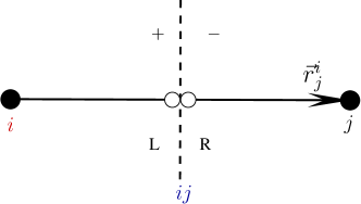
Figure 3: A satellite $j$, midpoint $ij$ and the centre $i$ in the cloud

The formulae from (16) to (21) provide a way to compute the spatial derivatives within a cloud of points. The Euler equations are required to be satisfied for every cloud of points in the domain. For any cloud $C_{i}$, Eq. (1) can be written as

$$\left.\frac{\partial\mathbf{U}}{\partial t}\right|_{C_{i}}+\left(\frac{\partial\mathbf{E}}{\partial x}+\frac{\partial\mathbf{F}}{\partial y}\right)_{C_{i}}=0$$ (23)

For simplicity, the subscript $i$ is used to represent the cloud $C_{i}$ in the following. Substitute Eq. (21) into Eq. (23) and it becomes

$$\frac{\partial\mathbf{U}_{i}}{\partial t}+\sum^{M_{i}}_{j=1}\left[\left(\alpha_{ij}\mathbf{E}_{ij}+\beta_{ij}\mathbf{F}_{ij}\right)-\left(\alpha_{ij}\mathbf{E}_{i}+\beta_{ij}\mathbf{F}_{i}\right)\right]=0$$ (24)

In order to calculate the flux terms in a non-split manner, the above equation needs to be expressed in a compact form. For this purpose, a parameter $\lambda$ defined as

$$\lambda=\sqrt{\alpha^{2}+\beta^{2}}$$ (25)

and a vector $\vec{\eta}=(\eta_{x},\eta_{y})$ estimated by

$$\eta_{x}=\frac{\alpha}{\lambda},\quad\eta_{y}=\frac{\beta}{\lambda}$$ (26)

are introduced to Eq. (24). Now it can be written in the following form

$$\frac{\partial\mathbf{U}_{i}}{\partial t}+\sum^{M_{i}}_{j=1}(\mathbf{G}_{ij}-\mathbf{G}_{i})\lambda_{ij}=0$$ (27)

where

$$\mathbf{{G}}=\eta_{x}\mathbf{E}+\eta_{y}\mathbf{F}=\begin{bmatrix}\rho q\\ \rho uq+p\eta_{x}\\ \rho vq+p\eta_{y}\\ (\rho e_{\rm t}+p)q\end{bmatrix}$$ (28)

in which $q$ is the dot product of $\vec{V}$ and $\vec{\eta}$

$$q=u\cdot\eta_{x}+v\cdot\eta_{y}$$ (29)

Modern programming languages such as Fortran 90/95 provide advanced array operations, which makes it easy for the computer codes be optimised on a machine with vector processors. Based on these considerations, the flux term is advised to be computed by the following vectorised formula

$$\mathbf{{G}}=q\mathbf{U}+p\mathbf{N}_{q}$$ (30)

where $\mathbf{N}_{q}=[0,\eta_{x},\eta_{y},q]^{\rm T}$.

As illustrated in Fig. 3, the flux function $\mathbf{G}$ at the midpoint $P_{ij}$ is evaluated by

$$\mathbf{G}_{ij}=\mathbf{G}(\mathbf{U}_{ij}^{\rm L},\mathbf{U}_{ij}^{\rm R})$$ (31)

A simple method to calculate the conservative variables for the left side L and the right side R is

$$\mathbf{U}_{ij}^{\rm L}=\mathbf{U}_{i},\quad\mathbf{U}_{ij}^{\rm R}=\mathbf{U}_{j}$$ (32)

This is the classical first-order Godunov scheme, which assumes a piecewise constant distribution of the flow variables. To improve the accuracy, a piecewise linear reconstruction of the data is adopted in this research. When reconstructing the data, one option is to choose the conservative variables, another is to reconstruct the characteristic variables and the other way is to select the primitive variables. In the present work, the data is reconstructed with the primitive variables $\mathbf{W}=(\rho,u,v,p)$ due to its simplicity compared to the conservative and characteristic variables

$$\mathbf{W}_{ij}^{L}=\mathbf{W}_{i}+\frac{1}{2}\nabla\mathbf{W}_{i}\cdot\mathbf{r}_{j}^{i}$$ (33a)

$$\mathbf{W}_{ij}^{R}=\mathbf{W}_{j}-\frac{1}{2}\nabla\mathbf{W}_{j}\cdot\mathbf{r}_{j}^{i}$$ (33b)

As high order schemes tend to produce spurious oscillations in the vicinity of large gradients [1], a slope or flux limiter needs to be used to satisfy the TVD constrains [39]. In the present work, the following slope limiter is employed

$$\varphi^{\rm L} =\frac{\nabla\mathbf{W}_{i}\cdot\vec{{r}}_{j}^{i}\Delta\mathbf{W}_{j}^{i}+\left|\nabla\mathbf{W}_{i}\cdot\vec{{r}}_{j}^{i}\Delta\mathbf{W}_{j}^{i}\right|+\epsilon}{(\nabla\mathbf{W}_{i}\cdot\vec{{r}}_{j}^{i})^{2}+(\Delta\mathbf{W}_{j}^{i})^{2}+\epsilon}$$ (34a)

$$\varphi^{\rm R} =\frac{\nabla\mathbf{W}_{k}\cdot\vec{{r}}_{j}^{i}\Delta\mathbf{W}_{j}^{i}+\left|\nabla\mathbf{W}_{k}\cdot\vec{{r}}_{j}^{i}\Delta\mathbf{W}_{j}^{i}\right|+\epsilon}{(\nabla\mathbf{W}_{k}\cdot\vec{{r}}_{j}^{i})^{2}+(\Delta\mathbf{W}_{j}^{i})^{2}+\epsilon}$$ (34b)

where $\Delta\mathbf{W}_{j}^{i}=\mathbf{W}_{j}-\mathbf{W}_{i}$. The small value $\epsilon$ is introduced to prevent null division in the smooth regions where differences approach zero, it is set as $\epsilon=10^{-12}$ in this research. In summary, the conservative variables are estimated by the reconstructed primitive variables

$$\mathbf{W}_{ij}^{L}=\mathbf{W}_{i}+\frac{1}{2}\varphi^{\rm L}\nabla\mathbf{W}_{i}\cdot\mathbf{r}_{j}^{i}$$ (35a)

$$\mathbf{W}_{ij}^{R}=\mathbf{W}_{j}-\frac{1}{2}\varphi^{\rm R}\nabla\mathbf{W}_{j}\cdot\mathbf{r}_{j}^{i}$$ (35b)

$$\mathbf{U}_{ij}^{\rm L,R}=\mathbf{U}(\mathbf{W}_{ij}^{\rm L,R})$$ (35c)

3.3 The HLLC approximate Riemann solver

Figure 4: The HLLC Riemann solver

As mentioned in Section 1, the HLLC Riemann solver introduces an intermediate contact wave to the original two-wave model of the HLL Riemann solver. Consequently, there are two intermediate averaged states ($\mathbf{U}_{\rm L}^{*}$ and $\mathbf{U}_{\rm R}^{*}$) separated by the contact wave $S_{\rm M}$ as shown in Figure 4. The approximate solution may be expressed by four averaged states

$$\mathbf{U}_{ij}=\left\{\begin{array}[]{ll}\mathbf{U}_{\rm L}&0\leq S_{\rm L}\\ \mathbf{U}_{\rm L}^{*}&0\in(S_{\rm L},S_{\rm M}]\\ \mathbf{U}_{\rm R}^{*}&0\in(S_{\rm M},S_{\rm R})\\ \mathbf{U}_{\rm R}&0\geq S_{\rm R}\end{array}\right.$$ (36)

The corresponding midpoint flux is given by

$$\mathbf{G}_{ij}=\left\{\begin{array}[]{ll}\mathbf{G}_{\rm L}&0\leq S_{\rm L}\\ \mathbf{G}_{\rm L}^{*}&0\in(S_{\rm L},S_{\rm M}]\\ \mathbf{G}_{\rm R}^{*}&0\in(S_{\rm M},S_{\rm R})\\ \mathbf{G}_{\rm R}&0\geq S_{\rm R}\end{array}\right.$$ (37)

Following the strategy of Toro [1] by applying the Rankine-Hugoniot conditions across the wave speeds $S_{\rm L}$ and $S_{\rm R}$, the following important formulations are obtained

$$\mathbf{G}_{\rm L}^{*}=\mathbf{G}_{\rm L}+S_{\rm L}^{*}(\mathbf{U}_{\rm L}^{*}-\mathbf{U}_{\rm L})$$ (38a)

$$\mathbf{G}_{\rm R}^{*}=\mathbf{G}_{\rm R}+S_{\rm R}^{*}(\mathbf{U}_{\rm R}^{*}-\mathbf{U}_{\rm R})$$ (38b)

In order to compute the intermediate state flux, the averaged state conservative flow variables are necessary. To provide these information, the intermediate flux is assumed to be a function of the averaged state flow variables as suggested by Batten et al. [8, 9]

$$\mathbf{G}_{\rm L}^{*}=q_{\rm L}^{*}\mathbf{U}_{\rm L}^{*}+p_{\rm L}^{*}\mathbf{N}_{q_{\rm L}^{*}}$$ (39a)

$$\mathbf{G}_{\rm R}^{*}=q_{\rm R}^{*}\mathbf{U}_{\rm R}^{*}+p_{\rm R}^{*}\mathbf{N}_{q_{\rm R}^{*}}$$ (39b)

Substitute Eq. (38) into the above equation, we obtain

$$(q_{\rm L}^{*}-S_{\rm L}^{*})\mathbf{U}_{\rm L}^{*}=\mathbf{G}_{\rm L}-S_{\rm L}^{*}\mathbf{U}_{\rm L}^{*}-p_{\rm L}^{*}\mathbf{N}_{q_{\rm L}^{*}}$$ (40a)

$$(q_{\rm R}^{*}-S_{\rm R}^{*})\mathbf{U}_{\rm R}^{*}=\mathbf{G}_{\rm R}-S_{\rm R}^{*}\mathbf{U}_{\rm R}^{*}-p_{\rm R}^{*}\mathbf{N}_{q_{\rm R}^{*}}$$ (40b)

Notice that $\mathbf{G}_{\rm L}$ and $\mathbf{G}_{\rm R}$ can be estimated by Eq. (30) straightforwardly,

$$\mathbf{G}_{\rm L}=q_{\rm L}\mathbf{U}_{\rm L}+p_{\rm L}\mathbf{N}_{q_{\rm L}}$$ (41a)

$$\mathbf{G}_{\rm R}=q_{\rm R}\mathbf{U}_{\rm R}+p_{\rm R}\mathbf{N}_{q_{\rm R}}$$ (41b)

Substitute Eq. (41) to (40), we obtain

$$\mathbf{U}_{\rm L}^{*}=\frac{(q_{\rm L}-S_{\rm L})\mathbf{U}_{\rm L}+(p_{\rm L}\mathbf{N}_{q_{\rm L}}-p_{\rm L}^{*}\mathbf{N}_{q_{\rm L}^{*}})}{q_{\rm L}^{*}-S_{\rm L}}$$ (42)

and

$$\mathbf{U}_{\rm R}^{*}=\frac{(q_{\rm R}-S_{\rm R})\mathbf{U}_{\rm R}+(p_{\rm R}\mathbf{N}_{q_{\rm R}}-p_{\rm R}^{*}\mathbf{N}_{q_{\rm R}^{*}})}{q_{\rm R}^{*}-S_{\rm R}}$$ (43)

Once the intermediate velocity component $q_{\rm L,R}^{*}$ and pressure $p_{\rm L,R}^{*}$ are known, the conservative variables can be easily obtained by the above two equations. Based on the condition

$$p_{\rm M}=p_{\rm L}^{*}=p_{\rm R}^{*}$$ (44)

(there is no jump of pressure across the contact wave) and a convenient assumption [8] setting the contact wave speed to the following

$$S_{\rm M}=q_{\rm L}^{*}=q_{\rm R}^{*}=q_{\rm M}$$ (45)

the intermediate wave speed can be calculated by

$$S_{\rm M}=\frac{\rho_{\rm R}q_{\rm R}(S_{\rm R}-q_{\rm R})-\rho_{\rm L}q_{\rm L}(S_{\rm L}-q_{\rm L})+p_{\rm L}-p_{\rm R}}{\rho_{\rm r}(S_{\rm R}-q_{\rm R})-\rho_{\rm L}(S_{\rm L}-q_{\rm L})}$$ (46)

and the intermediate pressure may be estimated as

$$p_{\rm M}=\rho_{\rm L}(q_{\rm L}-S_{\rm L})(q_{\rm L}-S_{\rm M})+p_{\rm L}=\rho_{\rm R}(q_{\rm R}-S_{\rm R})(q_{\rm R}-S_{\rm M})+p_{\rm R}$$ (47)

The left and right states wave speeds are computed by

$$S_{\rm L}=\min(q_{\rm L}-c_{\rm L},\tilde{q}-\tilde{c})$$ (48)

and

$$S_{\rm R}=\max(q_{\rm R}+c_{\rm R},\tilde{q}+\tilde{c})$$ (49)

where $\tilde{q}$ is an averaged velocity component evaluated by

$$\tilde{u}=\frac{\sqrt{\rho_{\rm L}}u_{\rm L}+\sqrt{\rho_{\rm R}}u_{\rm R}}{\sqrt{\rho_{\rm L}}+\sqrt{\rho_{\rm R}}}$$ (50a)

$$\tilde{v}=\frac{\sqrt{\rho_{\rm L}}v_{\rm L}+\sqrt{\rho_{\rm R}}v_{\rm R}}{\sqrt{\rho_{\rm L}}+\sqrt{\rho_{\rm R}}}$$ (50b)

$$\tilde{q}=\eta_{x}\tilde{u}+\eta_{y}\tilde{v}$$ (50c)

For ideal gas, the averaged speed of sound $\tilde{c}$ can be computed from the averaged enthalpy $\tilde{h}$ as stated by Roe [40] and Batten et al. [8, 9]

$$\tilde{h}=\frac{\sqrt{\rho_{\rm L}}h_{\rm L}+\sqrt{\rho_{\rm R}}h_{\rm R}}{\sqrt{\rho_{\rm L}}+\sqrt{\rho_{\rm R}}}$$ (51a)

$$\tilde{c}=\sqrt{(\gamma-1)\left[\tilde{h}-\frac{1}{2}(\tilde{u}^{2}+\tilde{v}^{2})\right]}$$ (51b)

However, it is not clear whether this also stands for compressible liquids with SG-EOS (4) as the corresponding formulations were not provided in their papers. Therefore, effort is made here to remove the ambiguity. To clarify this point, the relation between the enthalpy and speed of sound needs to be understood

$$\rho h=(\rho e_{\rm t}+p)$$ (52)

Substitue Eq. (3) and (4) into Eq. (52) then divided it by $\rho$, we obtain

$$h =(\rho e_{\rm t}+p)/\rho$$ (53a)

$$=\frac{1}{\gamma-1}\frac{\gamma}{\rho}(p+p_{\rm c})+\frac{1}{2}(u^{2}+v^{2})$$ (53b)

Substitue Eq. (5) into Eq. (53), we get

$$h=\frac{1}{\gamma-1}c^{2}+\frac{1}{2}(u^{2}+v^{2})$$ (54)

Therefore, the averaged speed of sound for compressible liquids can also be appropriately recovered from the averaged enthalpy given by Eq. (51).

Substitute Eq. (44), (45), (46) and (47) to Eq. (39), the intermediate left and right states flux can be expressed by the following forms

$$\mathbf{G}_{\rm L}^{*}=S_{\rm M}\mathbf{U}_{\rm L}^{*}+p_{\rm M}\mathbf{N}_{S_{\rm M}}$$ (55a)

$$\mathbf{G}_{\rm R}^{*}=S_{\rm M}\mathbf{U}_{\rm R}^{*}+p_{\rm M}\mathbf{N}_{S_{\rm M}}$$ (55b)

where $\mathbf{N}_{S_{\rm M}}=[0,\eta_{x},\eta_{y},S_{\rm M}]^{\rm T}$. When programming the practical code on a computer, we separate the process into two steps. Firstly, we need to estimate the three wave speeds (the left wave, right wave and intermediate contact wave). Then we compute the flux as Eq (37) according to the relations of these wave speeds. The whole procedure to evaluate $\mathbf{G}_{ij}$ is summarised in Algorithm 1.

Input : $\mathbf{U}_{\rm L},\mathbf{U}_{\rm R}$, $\vec{\eta}$

Output : $\mathbf{G}$

begin Wave speeds estimate

       $\mathbf{W}_{\rm L}\longleftarrow\mathbf{U}_{\rm L}$;

       $\mathbf{W}_{\rm R}\longleftarrow\mathbf{U}_{\rm R}$;

       $\tilde{q},\tilde{c}\longleftarrow\mathbf{W}_{\rm L},\mathbf{W}_{\rm R}$;

       $S_{\rm L}\longleftarrow$ Eq. (48) ;

       $S_{\rm R}\longleftarrow$ Eq. (49);

       $S_{\rm M}\longleftarrow$ Eq. (46);

       $p_{\rm M}\longleftarrow$ Eq. (47);

      

end

begin Flux determination

       if $0<S_{\rm L}$ then

            $\mathbf{G}=\mathbf{G}_{\rm L}\longleftarrow$ Eq. (41a);

       else if $S_{\rm L}\leq 0<S_{\rm M}$ then

             $\mathbf{U}_{\rm L}^{*}\longleftarrow$ Eq. (42) ;

             $\mathbf{G}=\mathbf{G}_{\rm L}^{*}\longleftarrow$ Eq. (55a) ;

       else if $S_{\rm M}\leq 0<S_{\rm R}$ then

             $\mathbf{U}_{\rm R}^{*}\longleftarrow$ Eq. (43) ;

             $\mathbf{G}=\mathbf{G}_{\rm R}^{*}\longleftarrow$ Eq. (55b) ;

       else

            $\mathbf{G}=\mathbf{G}_{\rm R}\longleftarrow$ Eq. (41b);

       end if

      

end

Algorithm 1 Non-split meshless HLLC Riemann solver

3.4 Temporal discretisation

In the present work, the Euler equations are treated by the method-of-line, which separates the temporal and spatial spaces. The semi-discrete form of the governing equations is given by

$$\frac{{\rm d}\mathbf{U}}{{\rm d}t}=\mathbf{R}$$ (56)

where $\mathbf{R}$ represents the residual. For cloud $i$, a forward difference discretisation of Eq. (56) is

$$\frac{\mathbf{U}^{n+1}_{i}-\mathbf{U}^{n}_{i}}{\Delta t}=\mathbf{R}_{i}$$ (57)

An explicit four-stage Runge-Kutta scheme is applied to update the solution from time level $n$ to $n+1$,

$$\mathbf{U}^{(0)}_{i}=\mathbf{U}^{n}_{i}$$ (58a)

$$\mathbf{U}^{(1)}_{i}=\mathbf{U}^{(0)}_{i}+\alpha_{1}\Delta t_{i}\mathbf{R}^{(0)}_{i}$$ (58b)

$$\mathbf{U}^{(2)}_{i}=\mathbf{U}^{(0)}_{i}+\alpha_{2}\Delta t_{i}\mathbf{R}^{(1)}_{i}$$ (58c)

$$\mathbf{U}^{(3)}_{i}=\mathbf{U}^{(0)}_{i}+\alpha_{3}\Delta t_{i}\mathbf{R}^{(2)}_{i}$$ (58d)

$$\mathbf{U}^{(4)}_{i}=\mathbf{U}^{(0)}_{i}+\alpha_{4}\Delta t_{i}\mathbf{R}^{(3)}_{i}$$ (58e)

$$\mathbf{U}^{n+1}_{i}=\mathbf{U}^{(4)}_{i}$$ (58f)

where $\alpha_{1}=\tfrac{1}{4}$, $\alpha_{2}=\tfrac{1}{3}$, $\alpha_{3}=\tfrac{1}{2}$ and $\alpha_{4}=1$ are the stage coefficients.

4 Numerical results

In order to validate the meshless HLLC approximate Riemann solver proposed in this paper, Toro’s one-dimensional gas shock tube problem is chosen as the first benchmark test. The method’s capability to deal with the compressible water in a liquid shock tube is also inspected (Except this test, all the other cases are compressible gas flow problems). Then more complicated two-dimensional problems including moving shock passing a cylinder, internal supersonic flows in channels and external transonic flows over aerofoils are examined. All the following numerical simulations are performed on a Compaq Presario-CQ45 laptop equipped with a dual-core P4 2.16GHz CPU, 1GB memory and 250GB hard drive. The main operating system on the laptop is Windows Vista (32bit), but the computation is run under Cygwin, which provides a Linux like environment. The underlying serial computing programs are written in Fortran 90 language and compiled by the GNU Fortran compiler. In this work, the finite volume method is employed together with the JST scheme, which is based on a central differencing with second order and fourth order artificial dissipation [42], to produce the reference results.

4.1 Gas shock tube

Toro’s shock tube, of which the mathematical model is the one-dimensional Euler equations, is chosen as the first test case. Although it is only a 1D problem, the exact solution is quite complicated as it consists of a shock wave, a contact discontinuity and a rarefaction. It provides a critical examination of the numerical method’s capability to resolve these complex physical features. The tube is filled with ideal gases of different states separated by an imaginary barrier imposed at the centre initially. The density, velocity and pressure of the gases at the initial state are given by

$$\mathbf{W}=\left\{\begin{array}[]{lr}(1,0.75,1)&-0.5\leq x\leq 0\\ (0.125,0,0.1)&0<x\leq 0.5\end{array}\right.$$ (59)

Figure 5: Initial condition setup for the gas shock tube

Transmissive boundary conditions are applied at $x=-0.5$ and $0.5$. Four hundred meshless points are used to divide the shock tube uniformly and the solution is computed to $t=0.2$. Both the first order Godunov scheme and piecewise linear reconstruction strategy are used to obtain the numerical results. The exact solution is produced by the computer program listed in Chapter 4 of Toro’s book [1]. The program utilises an iterative guess-correction (Newton-Raphson) strategy to find the exact solution, while ten thousands mesh points are used to depict the exact solution in the present work. The initial condition setup is illustrated in Figure 5. The density, velocity, pressure and density-averaged internal energy of the numerical and exact solutions are plotted in Figure 6, in which the solid line represents the exact solution, the dashed line is the first order result and the circular symbol stands for second order result. It clearly shows that the contact discontinuity (at about $x=0.25$) is successfully captured by the meshless HLLC approximate Riemann solver. The second-order scheme provides a reasonable better resolution of the contact discontinuity than the first-order one. The shock wave (at about $x=0.4$) is also resolved well by the numerical method.

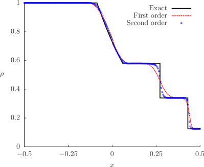
(a) density

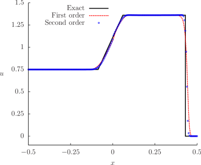
(b) velocity

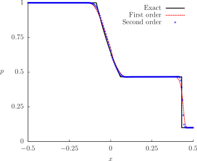
(c) pressure

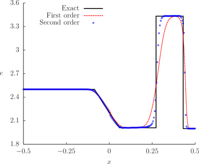
(d) internal energy

Figure 6: Gas shock tube

4.2 Liquid shock tube

The second test case is a liquid shock tube problem proposed by Ivings et al. [41]. The density, velocity and pressure of the liquids at the initial states are given by

$$\mathbf{W}=\left\{\begin{array}[]{lr}(1100,500,5\times 10^{9})&-0.5\leq x\leq 0\\ (1000,0,10^{5})&0<x\leq 0.5\end{array}\right.$$ (60)

Figure 7: Initial condition setup for the liquid shock tube

The polytropic constant is set to $\gamma=7.15$ and the pressure constant is taken as $p_{\rm c}=3\times 10^{8}$. The flow field is advanced to $t=6\times 10^{-5}$. The initial condition setup is shown in Figure 7. Figure 8 shows the exact solution and the numerical solutions. The exact solution is depicted by ten thousand points, the numerical solutions are obtained by the second order scheme for 100 and 400 meshless particles respectively. Obviously, the numerical method provides satisfactory results considering the wave speeds, locations and strengths.

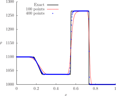
(a) density

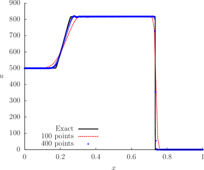
(b) velocity

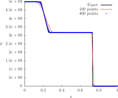
(c) pressure

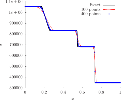
(d) internal energy

Figure 8: Liquid shock tube

After testing the numerical method for one-dimensional problems, we continue to benchmark the method for two-dimensional problems.

4.3 Moving shock passing a cylinder

This case was proposed by Luo et al. [32], in which an incident shock with $M_{s}=2$ is moving from the left side to the right side and passing a cylinder in a rectangular tube. The length of the tube is $6$ and its height is 3. The cylinder of radius $r=0.5$ is located at the centre of the tube. The number of the points distributed in the domain is $43,438$. The solution is advanced to $t=1.445$. Figure 9 exhibits the snapshots of the flow field at $t=0.6$, $0.9$, $1.2$ and $1.445$ with the density contours. Once the shock hits the cylinder ($t=0.6$), it is reflected to the left, upward and downward directions ($t=0.9\sim 1.2$). When the upward and downward reflected shocks touch the top and bottom boundaries of the tube, they are reflected again($t=1.445$). These complicated flow features are clearly shown in Figure 9. The present solution agrees well with the result of Luo et al. (Figure 19 of [32]).

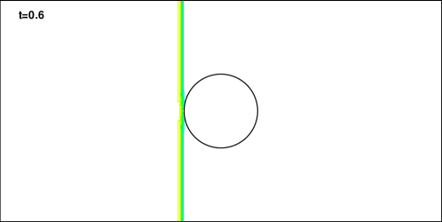
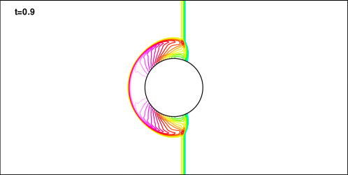
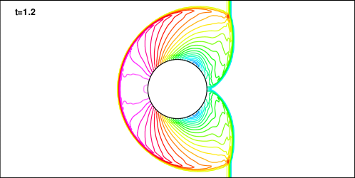
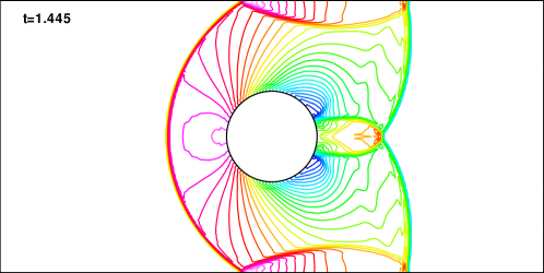
Figure 9: Moving shock wave passing a cylinder

4.4 Internal supersonic flow

Supersonic gas flow of $M_{\infty}=1.4$ in a channel with a $4\%$ circular bump is considered here. The length of the channel is $3$ and its height is $1$, the circular bump is located at the centre of the bottom boundary of the channel. The number of the points in the domain is $19,517$. The solution is started with the uniform supersonic flow and then advanced by the four-stage explicit Runge-Kutta method to the steady state. Besides the meshless method, we also compute the solution with the finite volume method for the purpose of comparison. The results of FVM and LSMM are shown in Figure 10. Inspecting the Mach number contours, it is not difficult to find that the flow features captured by LSMM are identical to those captured by FVM. The FVM solution exhibits strong oscillations near the shocks while LSMM result avoids these as shown in Figure 10 (c), which depicts the pressure coefficients on the top and bottom boundaries of the channel.

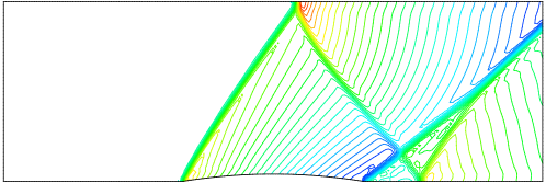
(a) Mach number contours - FVM

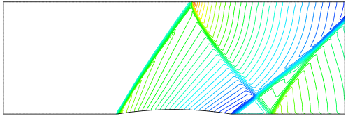
(b) Mach number contours - LSMM

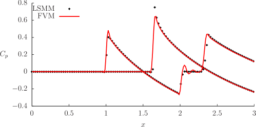
(c) Pressure coefficient

Figure 10: Supersonic flow in a tube with a $4\%$ circular bump, $M_{\infty}=1.4$

4.5 Transonic flows over the NACA0012 aerofoil

Two groups of transonic flows over the symmetric NACA0012 aerofoil with different flow conditions are chosen. The flow conditions for the first set are $M_{\infty}=0.8$ and $\alpha=0^{\rm o}$. For the second set, they are $M_{\infty}=0.8$ and $\alpha=1.25^{\rm o}$.

The number of meshless points in the flow domain is 5,557, while there are 42 points on the far field boundary and 310 nodes on the wall boundary. The natural neighbours around every point are chosen to form the meshless clouds. Due to the random property of the point distribution, the number of satellites for each cloud are not the same. For this case, the maximum number of satellites is 9, the minimum value is 4 and more than ninety percent of the clouds have six or seven satellites. Figure 11 exhibits the scattered points around the NACA0012 aerofoil.

The physical domain is initialised with uniform flows with the corresponding Mach number and angle of attack. Then the numerical solution starts with the impulse posed by the aerofoil. Local time stepping is applied to enhance the convergence rate to obtain the steady flows.

Figure 14 shows the Mach number contours in the flow field for these two-group tests. The first row presents the results of the zero-angle-of-attack and the second row give the results for $\alpha=1.25^{\rm o}$. We organise the FVM solution in the left column and the LSMM solution in the right column. For the case of zero-angle-of-attack, two strong shock waves symmetric about the aerofoil chord ($x$-axis) appear in the flow field, the locations of the shock wave are at the half chord. For $\alpha=1.25^{\rm o}$, a strong shock appears in the upper part of the domain and a relatively weak shock appears in the lower part of the field. The LSMM solution and FVM solution are almost the same as displayed in 14.

More details can be found when we look at Figure 12, in which the pressure coefficients around the aerofoil are depicted. The LSMM solutions are in good agreement with the FVM and other reference results (Jameson et al. [42], Pulliam and Stegeret [43] and Luo et al [44]) not only in smooth regions but also in regions with large gradients. The entropy productions on the aerofoil by FVM and LSMM are shown in Fig. 13. For these two cases, it seems that LSMM performs slightly better at the leading edge as it gives smaller entropy productions than FVM does.

Figure 11: Meshless points distribution around the NACA0012 aerofoil

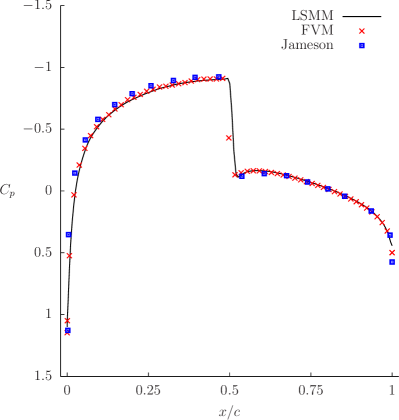
(a) $M_{\infty}=0.8$, $\alpha=0^{\rm o}$

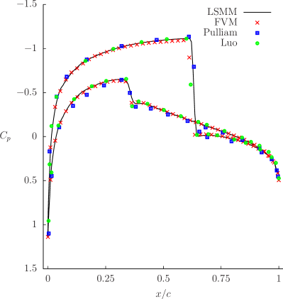
(b) $M_{\infty}=0.8$, $\alpha=1.25^{\rm o}$

Figure 12: Pressure coefficient around the NACA0012 aerofoil

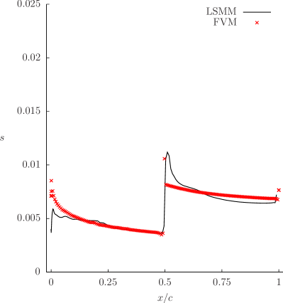
(a) $M_{\infty}=0.8$, $\alpha=0^{\rm o}$

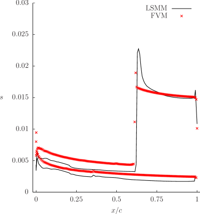
(b) $M_{\infty}=0.8$, $\alpha=1.25^{\rm o}$

Figure 13: Entropy production around the NACA0012 aerofoil

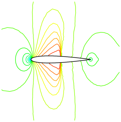
(a) $M_{\infty}=0.8$, $\alpha=0^{\rm o}$ - FVM

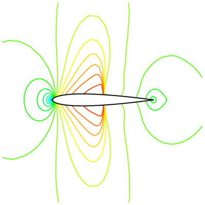
(b) $M_{\infty}=0.8$, $\alpha=0^{\rm o}$ - LSMM

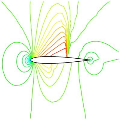
(c) $M_{\infty}=0.8$, $\alpha=1.25^{\rm o}$ - FVM

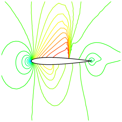
(d) $M_{\infty}=0.8$, $\alpha=1.25^{\rm o}$ - LSMM

Figure 14: Mach number contours for the NACA0012 aerofoil

4.6 Transonic flow over the RAE2822 aerofoil

For the RAE2822 aerofoil, we compute the transonic flow with the conditions $M_{\infty}=0.73$ and $\alpha=2.8^{\rm o}$. The number of meshless points in the domain is 5,482, there are 42 nodes on the far field boundary and 335 points on the wall boundary. Figure 15 is a snapshot of the scattered points around the RAE2822 aerofoil. The clouds of points are also constructed by the natural-neighbour selection criteria. The maximum number of satellite is 9 and the minimum value is 4 in the whole domain. The Mach number contours from the numerical solutions are shown in Figure 17, good agreement between the FVM and LSMM results is observed once more. The pressure coefficients around the aerofoil are shown in Figure 16(a), in which the result computed by a high-order discontinuous Galerkin method (DGM) from Luo et al. [44] is also included. DGM, FVM and LSMM all underestimate the pressure coefficient at the leading edge and overestimate at the trailing edge compared to the experiment [45]. The suction peaks captured by DGM, LSMM and FVM on the aerofoil upper surface adjacent to the leading are close to the laboratory data. DGM, FVM and LSMM get the same shock position, while DGM produces a stronger shock than FVM and LSMM. The shock waves captured by DGM, FVM and LSMM are all stronger than the experimental result and the location is behind the experiment. This is due to the lack of physical viscosity in the Euler equations for inviscid flows. In general, DGM, FVM and LSMM solutions agree reasonably well with the experimental data in smooth regions. The entropy productions on the aerofoil surface by FVM and LSMM are depicted in Fig. 16

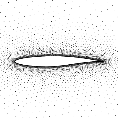
Figure 15: Meshless points distribution around the RAE2822 aerofoil

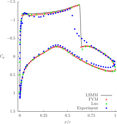
(a) Pressure coefficient

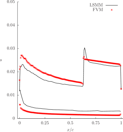
(b) Entropy production

Figure 16: Pressure coefficient and entropy production around the RAE2822 aerofoil

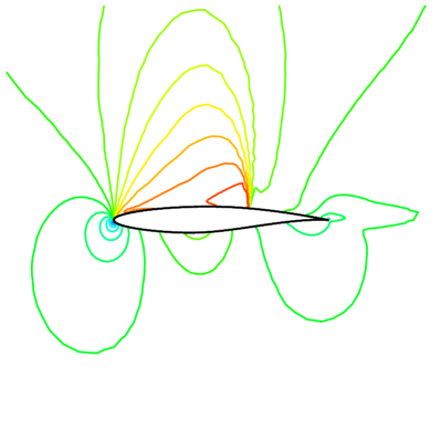
(a) FVM

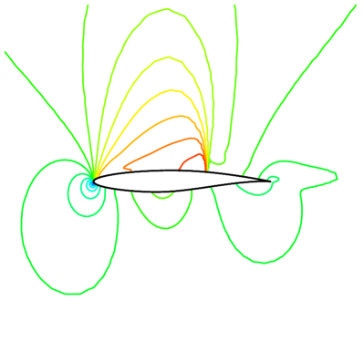
(b) LSMM

Figure 17: Mach number contours for the RAE2822 aerofoil

5 Conclusions

A meshless method with the HLLC Riemann solver for compressible flows is presented in this paper. The spatial derivatives of the Euler equations are discretised by the least-square scheme and the midpoint flux terms are computed by the appropriate HLLC Riemann solver for LSMM. Crucial information of the numerical method is derived and exposed in this paper with a step-by-step instructive computer algorithm provided to readers. Detailed comparisons with the available exact, finite volume and other reference results for various numerical test cases validate the methodology for gas flows. The attempt to handle compressible liquid flows with the proposed method gets unexpected positive feedback from the one-dimensional liquid shock tube test. Future work will include the development of the present method for solving compressible gas flow problems with moving boundaries and complicated two-/three-dimensional compressible liquid flows.

References

- [1] E. Toro, Riemann solvers and numerical methods for fluid dynamics: a practical introduction, Springer, 1997.
- [2] P. D. Lax, Hyperbolic Systems of Conservation Laws and the Mathematical Theory of Shock Waves, SIAM, 1973.
- [3] R. J. LeVeque, Finite Volume Methods for Hyperbolic Problems, Randall J. LeVeque, 2002.
- [4] J. D. Anderson, Computational Fluid Dynamics. The Basics with Applications., McGraw-Hill, 1995.
- [5] A. Harten, P. D. Lax, B. van Leer, On upstream differencing and Godunov–type schemes for hyperbolic conservation laws, SIAM Review 25 (1983) 35–61.
- [6] E. F. Toro, M. Spruce, W. Speares, Restoration of the contact surface in the HLL- Riemann solver, Tech. rep., Cranfield Institute of Technology (1992).
- [7] E F Toro, M Spruce and W Speares. Restoration of the contact surface in the Harten-Lax-van Leer Riemann solver, Shock Waves 4(1994) 25–34.
- [8] P. Batten, N. Clarke, C. Lambert, D. Causon, On the choice of wavespeeds for the HLLC Riemann solver, SIAM Journal on Scientific Computing 18 (6) (1997) 1553–1570.
- [9] P. Batten, M. A. Leschziner, U. C. Goldberg, Average-state Jacobians and implicit methods for compressible viscous and turbulent flows, Journal Of Computational Physics 137 (1997) 38–78.
- [10] H. Luo, J. D. Baum, R. Löhner, On the computation of multi-material flows using ALE formulation, Journal of Computational Physics 194 (1) (2004) 304 – 328. doi:10.1016/j.jcp.2003.09.026.
- [11] X. Hu, N. Adams, G. Iaccarino, On the HLLC Riemann solver for interface interaction in compressible multi-fluid flow, Journal of Computational Physics 228 (17) (2009) 6572 – 6589. doi:10.1016/j.jcp.2009.06.002.
- [12] E. Johnsen, T. Colonius, Implementation of WENO schemes in compressible multicomponent flow problems, Journal of Computational Physics 219 (2) (2006) 715 – 732. doi:10.1016/j.jcp.2006.04.018.
- [13] R. Lagumbay, A. Haselbacher, O. Vasilyev, J. Wang, Numerical simulation of a high pressure supersonic multiphase jet flow through a gaseous medium, in: 2004 ASME International Mechanical Engineering Congress Expo, Vol. 1, 2004.
- [14] M. J. Ivings, D. M. Causon, E. F. Toro, On hybrid high resolution upwind methods for multicomponent flows, ZAMM - Journal of Applied Mathematics and Mechanics / Zeitschrift für Angewandte Mathematik und Mechanik 77 (9) (1997) 645–668. doi:10.1002/zamm.19970770904.
- [15] J. T. Batina, A gridless Euler/Navier-Stokes solution algorithm for complex-aircraft applications, in: 31st Aerospace Sciences Meeting & Exhibit, 1993, aIAA Paper 93-0333.
- [16] J. T. Batina, A gridless Euler/Navier-stokes solution algorithm for complex two-dimensional applications, Tech. rep., NASA Langley Research Center, nASA-TM-107631 (June 1992).
- [17] H. Q. Chen, C. Shu, An efficient implicit mesh-free method to solve two-dimensional compressible Euler equations, International Journal of Modern Physics C 16 (2005) 439–454. doi:10.1142/S0129183105007327.
- [18] A. Katz, A. Jameson, Multicloud: Multigrid convergence with a meshless operator, Journal of Computational Physics 228 (14) (2009) 5237 – 5250. doi:DOI:10.1016/j.jcp.2009.04.023.
- [19] D. J. Kirshman, F. Liu, A gridless boundary condition method for the solution of the Euler equations on embedded Cartesian meshes with multigrid, Journal of Computational Physics 201 (1) (2004) 119 – 147. doi:10.1016/j.jcp.2004.05.006.
- [20] E. P. C. Koh, H. M. Tsai, F. Liu, Euler solution using Cartesian grid with a gridless least-squares boundary treatment, AIAA JOURNAL 43 (2) (2005) 246–255.
- [21] Z. Ma, H. Chen, C. Zhou, A study of point moving adaptivity in gridless method, Computer Methods in Applied Mechanics and Engineering 197 (21-24) (2008) 1926–1937. doi:10.1016/j.cma.2007.12.012.
- [22] K. Morinishi, An implicit gridless type solver for the Navier-Stokes equations, Computational Fluid Dynamics Journal Special Issue (2001) 551–560.
- [23] D. Sridar, N. Balakrishnan, An upwind finite difference scheme for meshless solvers, Journal of Computational Physics 189 (1) (2003) 1–29. doi:10.1016/S0021-9991(03)00197-9.
- [24] P. Tota, Z. Wang, Meshfree Euler solver using local radial basis functions for inviscid compressible flows, in: 18th AIAA Computational Fluid Dynamics Conference, 2007, aIAA-2007-4581.
- [25] H. Wang, H.-Q. Chen, J. Periaux, A study of gridless method with dynamic clouds of points for solving unsteady CFD problems in aerodynamics, International Journal for Numerical Methods in Fluids 64 (1) (2010) 98–118. doi:10.1002/fld.2145.
- [26] Y. Hashemi, A. Jahangirian, Implicit fully mesh-less method for compressible viscous flow calculations, Journal of Computational and Applied Mathematics In Press, Corrected Proof (2010) 2. doi:10.1016/j.cam.2010.08.002.
- [27] E. Ortega, E. Oñate, S. Idelsohn, A finite point method for adaptive three-dimensional compressible flow calculations, International Journal for Numerical Methods in Fluids 60 (9) (2009) 937 – 971. doi:10.1002/fld.1892.
- [28] R. Löhner, C. Sacco, E. Oñate, S. Idelsohn, A finite point method for compressible flow, International Journal for Numerical Methods in Engineering 53 (8) (2002) 1765 – 1779. doi:10.1002/nme.334.
- [29] N. Munikrishna, N. Balakrishnan, Turbulent flow computations on a hybrid cartesian point distribution using meshless solver LSFD-U, Computers and Fluids 40 (1) (2011) 118 – 138. doi:10.1016/j.compfluid.2010.08.017.
- [30] H. Luo, J. Baum, R. Löhner, A hybrid building-block and gridless method for compressible flows, International journal for numerical methods in fluids 59 (4) (2009) 459–474. doi:10.1002/fld.1827.
- [31] H. Luo, J. Baum, R. Löhner, A hybrid cartesian grid and gridless method for compressible flows, in: 43rd AIAA Aerospace Sciences Meeting and Exhibit, 2005.
- [32] H. Luo, J. D. Baum, R. Löhner, A hybrid Cartesian grid and gridless method for compressible flows, Journal of Computational Physics 214 (2) (2006) 618 – 632. doi:10.1016/j.jcp.2005.10.002.
- [33] X. Zhou, H. Xu, Gridless method for unsteady flows involving moving discrete points and its applications, Engineering Applications of Computational Fluid Mechanics 4 (2010) 276 – 286.
- [34] J. Liu, S. Su, A potential gridless solution method for the compressible Euler/Navier-Stokes equations, in: 34th AIAA Aerospace Sciences Meeting and Exhibit, 1996, aIAA Paper 1996-0526.
- [35] E. Oñate, S. Idelsohn, O. Zienkiewicz, R. Taylor, A finite point method in computational mechanics. Applications to convective transport and fluid flow, International Journal for Numerical Methods in Engineering 39 (22) (1996) 3839 – 3866.
- [36] A. Katz, A. Jameson, A comparison of various meshless schemes within a unified algorithm, in: 47th AIAA Aerospace Sciences Meeting Including The New Horizons Forum and Aerospace Exposition, 2009, aIAA Paper 2009-596.
- [37] H. Q. Chen, An implicit gridless method and its applications, Acta Aerodynamica Sinica 20 (2) (2002) 133–140.
- [38] Z. Ma, H. Chen, X. Wu, A gridless-finite volume hybrid algorithm for Euler equations, Chinese Journal of Aeronautics 19 (4) (2006) 286–294.
- [39] A. Harten, High resolution schemes for hyperbolic conservation laws, Journal of Computational Physics 135 (2) (1997) 260 – 278. doi:10.1006/jcph.1997.5713.
- [40] P. Roe, Approximate Riemann solvers, parameter vectors, and difference schemes, Journal of Computational Physics 43 (2) (1981) 357 – 372. doi:10.1016/0021-9991(81)90128-5.
- [41] M. J. Ivings, D. M. Causon, E. F. Toro, On Riemann solvers for compressible liquids, International Journal for Numerical Methods in Fluids 28 (3) (1998) 395–418. doi:10.1002/(SICI)1097-0363(19980915)28:3<395::AID-FLD718>3.0.CO;2-S.
- [42] A. Jameson, W. Schmidt, E. Turkel, Numerical solutions of the Euler equations by finite volume methods using Runge-Kutta time-stepping schemes, AIAA paper 81 (1981) 1259.
- [43] T. Pulliam, J. Steger, Recent improvements in efficiency, accuracy, and convergence for implicit approximate factorization algorithms, in: AlAA 23rd Aerospace Sciences Meeting, Vol. 85, 1985, p. 0360.
- [44] H. Luo, J. D. Baum, R. Löhner, On the computation of steady-state compressible flows using a discontinuous Galerkin method, International Journal for Numerical Methods in Engineering 73 (5) (2008) 597–623. doi:10.1002/nme.2081.
- [45] P. H. Cook, M. C. P. Mcdonald, Aerofoil RAE2822 pressure distributions, and boundary layer and wake measurements[r] experimental data base for computer program assessment,, Tech. rep., AGARD, aR-138 (1979).
- [46] B. Godderidge, S. Turnock, C. Earl, M. Tan, The effect of fluid compressibility on the simulation of sloshing impacts, Ocean Engineering 36(2009) 578-587.
- [47] A. Murrone, H. Guillard, A five equation reduced model for compressible two phase flow problems, Journal of Computational Physics 202 (2005) 664–698.
- [48] E. Johnsen, T. Colonius, Implementation of WENO schemes in compressible multicomponent flow problems, Journal of Computational Physics 219 (2006) 715-732.
- [49] H. Bredmose, D. H. Peregrine, G. N. Bullock, Violent breaking wave impacts. Part 2: modelling the effect of air, Journal of Fluid Mechanics 641 (2009) 389–430.
- [50] L. Plumerault, D. Astruc, P. Villedieu, P. Maron, A numerical model for aerated-water wave breaking, International Journal for Numerical Methods in Fluids 69(2012) 1851–1871.
- [51] D. Causon, C. Mingham, Finite volume simulation of unsteady shock-cavitation in compressible water, International Journal for Numerical Methods in Fluids 72 (2013) 632–649.
- [52] S. Chenoweth, J. Soria, A. Ooi, A singularity-avoiding moving least squares scheme for two-dimensional unstructured meshes, Journal of Computational Physics 228 (2009) 5592-5619