arXiv preprint, February 2014

ACOUSTIC SPACE LEARNING FOR SOUND-SOURCE SEPARATION

AND LOCALIZATION ON BINAURAL MANIFOLDS

ANTOINE DELEFORGE

INRIA Grenoble Rhône-Alpes, 655 Avenue de l’Europe

Saint-Ismier, 38334, France

E-mail: antoine.deleforge@inria.fr

FLORENCE FORBES

INRIA Grenoble Rhône-Alpes, 655 Avenue de l’Europe

Saint-Ismier, 38334, France

E-mail: florence.forbes@inria.fr

RADU HORAUD

INRIA Grenoble Rhône-Alpes, 655 Avenue de l’Europe

Saint-Ismier, 38334, France

E-mail: radu.horaud@inria.fr

In this paper we address the problems of modeling the acoustic space generated by a full-spectrum sound source and of using the learned model for the localization and separation of multiple sources that simultaneously emit sparse-spectrum sounds. We lay theoretical and methodological grounds in order to introduce the binaural manifold paradigm. We perform an in-depth study of the latent low-dimensional structure of the high-dimensional interaural spectral data, based on a corpus recorded with a human-like audiomotor robot head. A non-linear dimensionality reduction technique is used to show that these data lie on a two-dimensional (2D) smooth manifold parameterized by the motor states of the listener, or equivalently, the sound source directions. We propose a probabilistic piecewise affine mapping model (PPAM) specifically designed to deal with high-dimensional data exhibiting an intrinsic piecewise linear structure. We derive a closed-form expectation-maximization (EM) procedure for estimating the model parameters, followed by Bayes inversion for obtaining the full posterior density function of a sound source direction. We extend this solution to deal with missing data and redundancy in real world spectrograms, and hence for 2D localization of natural sound sources such as speech. We further generalize the model to the challenging case of multiple sound sources and we propose a variational EM framework. The associated algorithm, referred to as variational EM for source separation and localization (VESSL) yields a Bayesian estimation of the 2D locations and time-frequency masks of all the sources. Comparisons of the proposed approach with several existing methods reveal that the combination of acoustic-space learning with Bayesian inference enables our method to outperform state-of-the-art methods.
Keywords: binaural hearing; sound localization; sound-source separation; manifold learning; mixture of regressors; EM inference.

1 Introduction

The remarkable abilities of humans to localize one or several sound sources and to identify their content from the perceived acoustic signals have been intensively studied in psychophysics^?, computational auditory analysis^?, and more recently in the emerging field of robot hearing^?. A classical example which illustrates the difficulty of understanding these human skills, is the well known cocktail party effect introduced by Cherry^? that still challenges today’s methods^?: How are listeners able to decipher speech in the presence of other sound sources, including competing talkers? While human listeners solve this problem routinely and effortlessly, this is still a challenge in computational audition.

There is behavioral and physiological evidence that human listeners use binaural cues in order to estimate the direction of a sound source^? and that sound localization plays an important role for solving the cocktail party problem^?,?. Two binaural cues seem to play an essential role, namely the interaural level difference (ILD) and the interaural time difference (ITD), or its spectral equivalent the interaural phase difference (IPD). Both ILD and IPD are known to be subject-dependent and frequency-dependent cues, due to the so-called head related transfer function (HRTF) generated by the shape of the head, pinna and torso, which filters signals arriving at each eardrum. These complex shapes induce a non-linear dependency of the HRTFs on the sound source direction^?,?. It is known that the spatial information provided by interaural-difference cues within a restricted band of frequency is spatially ambiguous, particularly along a roughly vertical and front/back dimension^?. This suggests that humans and mammals make use of full spectrum information for 2D sound source localization^?,?. This is confirmed by biological models of the auditory system hypothesizing the existence of neurons dedicated to the computation of interaural cues in specific frequency bands^?.

A lot of computational techniques exist to extract ITD, ILD and IPD from binaural recordings, either in the time domain using cross-correlation^?,?, or in the time-frequency domain using Fourier analysis^?,? or gammatone filters^?. However, the problem of localizing and/or separating several sound sources remains a challenge in computational auditory scene analysis, for several reasons. Firstly, the mapping from interaural cues to sound-source positions is usually unknown, complex and non-linear due to the transfer function of microphones which cannot be easily modeled. Secondly, auditory data are corrupted by noise and reverberations. Thirdly, an interaural value at a given frequency is relevant only if the source is actually emitting at that frequency: Natural sounds such as speech are known to be extremely sparse, with often 80% of the frequencies actually missing at a given time. Finally, when several sources emit simultaneously, the assignment of a time-frequency point to one of the sources is hard to estimate. The first problem, i.e., mapping audio cues to source positions, is central: Yet, it has received little attention in computational audition. Most existing approaches approximate this mapping based on simplifying assumptions, such as direct-path source-to-microphone propagation^?, a sine interpolation of ILD data from a human HRTF dataset^?, or a spiral ear model^?. These simplifying assumptions are often not valid in real world conditions. Following this view, accurately modeling a real world binaural system would require a prohibitively high number of parameters including the exact shape and acoustic properties of the recording device and of the room, which are unaccessible in practice. Due to this difficulty, the vast majority of current binaural sound localization approaches mainly focus on a rough estimation of a frontal azimuth angle, or one-dimensional (1D) localization^?,?,?,?, and very few perform 2D localization^?. Alternatively, some approaches^?,?,? bypass the explicit mapping model and perform 2D localization by exhaustive search in a large HRTF look-up table associating source directions to interaural spectral cues. However, this process is unstable and hardly scalable in practice as the number of required associations yields prohibitive memory and computational costs.

On the other hand, a number of psychophysical studies have suggested that the ability of localizing sounds is learned at early stages of development in humans and mammals^?,?,?. That is, the link between auditory features and source locations might not be hardcoded in the brain but rather learned from experience. The sensorimotor theory, originally laid by Poincaré^? and more recently investigated by O’Regan^?, suggests that experiencing the sensory consequences of voluntary motor actions is necessary for an organism to learn the perception of space. For example, Held and Hein^? showed that neo-natal kittens deprived of the ability of moving while seeing could not develop vision properly. Most notably, Aytekin et al.^? proposed a sensorimotor model of sound source localization using HRTF datasets of bats and humans. In particular, they argue that biological mechanisms could learn sound localization based solely on acoustic inputs and their relation to motor states.

In this article, we get inspiration from these psychological studies to propose a supervised learning computational paradigm for multiple sound source separation and localization. In other words, the acoustic properties of a system are first learned during a training phase. A key element of this study is the existence of binaural manifolds, which are defined and detailed in this article. Their existence is asserted through an in-depth study of the intrinsic structure of high-dimensional interaural spectral cues, based on real world recordings with a human-like auditory robot head. A non-linear dimensionality reduction technique is used to show that these cues lie on a two-dimensional (2D) smooth manifold parameterized by the motor states of the system, or equivalently, the sound source directions. With this key observation in mind, we propose a probabilistic piecewise affine mapping model (PPAM) specifically designed to deal with high-dimensional data presenting such a locally linear structure. We explain how the model parameters can be learned using a closed-form expectation-maximization (EM) procedure, and how Bayes inversion can be used to obtain the full posterior density function of a sound source direction given a new auditory observation. We also show how to extend this inversion to deal with missing data and redundancy in real world spectrograms, and hence for two-dimensional localization of natural sound sources such as speech. We further extend this inversion to the challenging case of multiple sound sources emitting at the same time, by proposing a variational EM (VEM) framework. The associated algorithm, referred to as variational EM for source separation and localization (VESSL) yields a Bayesian estimation of the 2D locations and time-frequency masks of all the sources. We introduced some parts of this paradigm in previous work^?,?, and we propose in this article a unified, more detailed and in-depth presentation of the global methodology.

The remainder of this article is organized as follows. Section 1.1 provides a brief literature overview of sound source separation and space mapping. Section 2 describes how interaural cues are computed in our framework. Section 3 presents the audio-motor dataset specifically recorded for this study. Section 4 describes the manifold learning method used to prove the existence of smooth binaural manifolds parameterized by source directions. Section 5 describes the PPAM model, its inference using EM, as well as the associated inverse mapping formula extended to missing and redundant observations in spectrograms. Section 6 further extends the inversion to the case of multiple sound sources with the VESSL algorithm. Section 7 shows detailed performance of PPAM and VESSL in terms of mapping, sound separation and sound localization under various conditions. Results are compared to state-of-the-art methods. Finally, Section 8 concludes and provides directions for future work.

1.1 Related work

Sound Source Separation. The problem of sound source separation has been thoroughly studied in the last decades and several interesting approaches have been proposed. Some methods^?,? achieve separation with a single microphone, based on known acoustic properties of speech signals, and are therefore limited to a specific type of input. Other techniques such as independent component analysis (ICA)^? require as many microphones as the number of sources. A recently explored approach is to use Gaussian complex models for spectrograms and estimate source parameters using an expectation-maximization algorithm^?. However, these methods are known to be very sensitive to initialization due to the large dimensionality of the parameter space, and often rely on external knowledge or other sound source separation algorithms for initialization.

Another category of methods uses binaural localization cues combined with time-frequency masking for source separation^?,?,?. Time-frequency masking, also called binary masking, allows the separation of more sources than microphones from a mixed signal, with the assumption that a single source is active at every time-frequency point. This is referred to as the W-disjoint orthogonality assumption^? and it has been shown to hold, in general, for simultaneous speech signals. Recently, Mandel et al.^? proposed a probabilistic model for multiple sound source localization and separation based on interaural spatial cues and binary masking. For each sound source, a binary mask and a discrete distribution over interaural time delays is provided. This can be used to approximate the frontal azimuth angle of the sound source using a direct-path sound propagation model, if the distance between the microphones is known.

Space Mapping. The task of learning a mapping between two spaces can be summarized as follows: if we are given a set of training couples $\{(\mbox{\boldmath$x$}_{n},\mbox{\boldmath$y$}_{n})\}_{n=1}^{N}\subset\mathbb{R}^{L}\times\mathbb{R}^{D}$, how can we obtain a relationship between $\mathbb{R}^{L}$ and $\mathbb{R}^{D}$ such that given a new observation in one space, its associated point in the other space is deduced? This problem has been extensively studied in machine learning, and offers a broad range of applications. In this study, we are interested in mapping a high-dimensional space to a low dimensional space, where the relationship between the two spaces is approximately locally linear. Indeed, it is showed in Section 4 that high dimensional spectral interaural data lie on a smooth Riemanian manifold, which by definition is locally homeomorphic to an Euclidean space. High-to-low-dimensional mapping problems are often solved in two steps, i.e., dimensionality reduction followed by regression. Methods falling into this category are partial least-squares^?, sliced inverse regression (SIR)^? and kernel SIR^?, but they are not designed to model local linearity. An attractive probabilistic approach for local linearity is to use a mixture of locally linear sub-models. A number of methods have explored this paradigm in the Gaussian case, such as mixture of linear regressors^?, mixture of local experts^? and methods based on joint Gaussian mixture models^?,?,?,? (GMM), that were recently unified in a common supervised and unsupervised mapping framework^?. Joint GMM has particularly been used in audio applications such as text-to-speech synthesis, voice conversion or articulatory-acoustic mapping systems. In Section 5, we propose a variant of the mixture of local experts model^? specifically adapted to locally linear and high-to-low dimensional mapping with an attractive geometrical interpretation. The concept of acoustic space learning introduced in this article, i.e., the idea of learning a mapping from interaural cues to 2D source positions and exploiting this mapping for sound source separation and localization does not seem to have been explored in the past.

2 Extracting Spatial Cues from Sounds

To localize sound sources, one needs to find a representation of sounds that 1) is independent of the sound source content, i.e., the emitted signal and 2) contains discriminative spatial information. These features can be computed in the time domain, but contain richer information when computed for different frequency channels, i.e., in the time-frequency domain. This section presents the time-frequency representation and spatial features used in this study.

2.1 Time-Frequency Representation

A time-frequency representation can be obtained either using Gammatone filter banks^?, which are mimicking human auditory representation, or short-term Fourier transform (STFT) analysis^?,?. The present study uses STFT as it is more directly applicable to source separation through binary-masking, as addressed in Section 6. First, the complex-valued spectrograms associated with the two microphones are computed with a 64 ms time-window and 8 ms hop, yielding $T=126$ frames for a 1 s signal. These values proved to be a good compromise between computational time and time-frequency resolution. Since sounds are recorded at 16,000 Hz, each time window contains 1,024 samples which are transformed into $F=512$ complex Fourier coefficients associated to positive frequency channels between 0 and 8,000 Hz. For a binaural recording made in the presence of a sound source located at $x$ in a listener-centered coordinate frame, we denote with $\{s^{(\textrm{S})}_{ft}\}_{f,t=1}^{F,T}$ the complex-valued spectrogram emitted by the source, and with $\{s^{(\textrm{L})}_{ft}\}_{f,t=1}^{F,T}$ and $\{s^{(\textrm{R})}_{ft}\}_{f,t=1}^{F,T}$ the left and right perceived spectrograms.

2.2 Interaural Spectral Cues

The HRTF model provides a relationships between the spectrogram emitted from source position $x$ and the perceived spectrograms:

$$\left\{\begin{array}[]{l}s^{(\textrm{L})}_{ft}=h_{f}^{(\textrm{L})}(\mbox{\boldmath$x$})\;s^{(\textrm{S})}_{ft}\\ s^{(\textrm{R})}_{ft}=h_{f}^{(\textrm{R})}(\mbox{\boldmath$x$})\;s^{(\textrm{S})}_{ft}.\end{array}\right.$$ (1)

where $\mbox{\boldmath$h$}^{(\textrm{L})}$ and $\mbox{\boldmath$h$}^{(\textrm{R})}$ denote the left and right non-linear HRTFs. The interaural transfer function (ITF) is defined by the ratio between the two HRTFs, i.e., $I_{f}(\mbox{\boldmath$x$})=h_{f}^{(\textrm{R})}(\mbox{\boldmath$x$})/h_{f}^{(\textrm{L})}(\mbox{\boldmath$x$})\in\mathbb{C}$. The interaural spectrogram is defined by $\hat{I}_{ft}=s^{(\textrm{R})}_{ft}/s^{(\textrm{L})}_{ft}$, so that $\hat{I}_{ft}=I_{f}(\mbox{\boldmath$x$})$. This way, $\hat{I}_{ft}$ does not depend on the emitted spectrogram value $s^{(S)}_{ft}$ but only on the emitting source position $x$. However, this equality holds only if the source is emitting at $(f,t)$ (i.e., $s^{(\textrm{S})}_{ft}\neq 0$). Since natural sounds have a null acoustic level at most time-frequency bins, associated interaural spectrograms will be very sparse, i.e., they will have many missing values. To characterize missing interaural spectrogram values, we introduce the binary variables $\chi_{ft}$ so that $\chi_{ft}=0$ if the value at $(f,t)$ is missing and $\chi_{ft}=1$ otherwise. They can be determined using a threshold on left and right spectral powers $|s^{(\textrm{L})}_{ft}|^{2}$ and $|s^{(\textrm{R})}_{ft}|^{2}$. We define the ILD spectrogram $\alpha$ and the IPD spectrogram $\phi$ as the log-amplitude and phase of the interaural spectrogram $\hat{I}_{f,t}$:

$$\left\{\begin{array}[]{l}\alpha_{ft}=20\log|\hat{I}_{ft}|\in\mathbb{R},\\ \phi_{ft}=\exp(j\arg(\hat{I}_{ft}))\in\mathbb{C}.\end{array}\right.$$ (2)

The phase difference is expressed in the complex domain, or equivalently $\mathbb{R}^{2}$, to avoid problems due to phase circularity. This way, two nearby phase values will be nearby in terms of Euclidean distance. In the particular case of a sound source emitting white noise from $x$, we have $\chi_{ft}=1$ for all $(f,t)$, i.e., the sound source is emitting at all $(f,t)$ points. One can thus compute the temporal means $\bar{\mbox{\boldmath$\alpha$}}\in\mathbb{R}^{F}$ and $\bar{\mbox{\boldmath$\phi$}}\in\mathbb{R}^{2F}$ of ILD and IPD spectrograms. These vectors will be referred to as the mean interaural vectors associated with $x$. The well established duplex theory^? suggests that ILD cues are mostly used at high frequencies (above 2 kHz) while ITD (or IPD) cues are mostly used at low frequencies (below 2 kHz) in humans. Indeed, ILD values are similar at low frequencies because the HRTF can be neglected, and the phase difference becomes very unstable with respect to the source position at high frequencies. To account for these phenomena, the initial binaural cues are split into two distinct vectors, namely the mean low-ILD and high-ILD and the mean low-IPD and high-IPD vectors, where low corresponds to frequency channels between 0 and 2 kHz and high corresponds to frequency channels between 2 kHz and 8 kHz. Frequency channels below 300 Hz were also removed in low-IPD vectors as they did not prove to contain significant information, due to a high amount of noise in this frequency range.

3 The CAMIL Dataset: Audiomotor Sampling of the Acoustic Space

We developed a technique to gather a large number of interaural vectors associated with source positions, in an entirely unsupervised and automated way. Sound acquisition is performed with a Sennheiser MKE 2002 acoustic dummy-head linked to a computer via a Behringer ADA8000 Ultragain Pro-8 digital external sound card. The head is mounted onto a robotic system with two rotational degrees of freedom: a pan motion and a tilt motion (see Fig. 1). This device is specifically designed to achieve precise and reproducible movements${}^{\mbox{\scriptsize a}}$. The emitter – a loud-speaker – is placed at approximately 2.7 meters ahead of the robot, as shown on Fig. 1. The loud-speaker’s input and the microphones’ outputs are handled by two synchronized sound cards in order to simultaneously record and play. All the experiments are carried out in real-world conditions, i.e., in a room with natural reverberations and background noise due to computer fans.

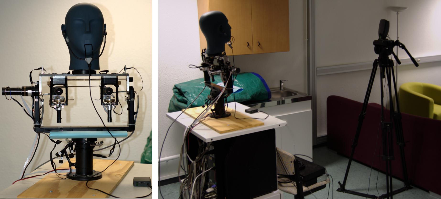
Fig. 1: A binaural dummy head is placed onto a motor system which can perform precise and reproducible pan and tilt motions (left). The emitter (a loud-speaker) is placed in front of the robot (right).

Rather than placing the emitter at known 3D locations around the robot, it is kept in a fixed reference position while the robot records emitted sounds from different motor states. Consequently, a sound source direction is directly associated with a pan-tilt motor state $(\psi,\theta)$. A great advantage of the audio-motor method is that it allows to obtain a very dense sampling of almost the entire acoustic space. The overall training is fully-automatic and takes around 15 hours, which could not be done manually. However, it also presents a limitation: A recording made at a given motor-state only approximates what would be perceived if the source was actually placed at the corresponding relative position in the room. This approximation holds only if the room has relatively few asymmetries and reverberations, which might not be the case in general. Note that when this is the case, a sound localization system trained with this dataset could be used to directly calculate the head movement pointing toward an emitting sound source. This could be done without needing inverse kinematics, distance between microphones or any other parameters. Alternatively, one could learn the room acoustics together with the system acoustics using, e.g., visual markers related to an emitter successively placed in different positions around the static head. Interestingly, the remainder of this study does not depend on the specific way source-position-to-interaural-cues associations are gathered.

Recordings are made from $10,800$ uniformly spread motor states covering the entire reachable motor-state space of the robot: $180$ pan rotations $\psi$ in the range $[-180^{\circ},180^{\circ}]$ (left-right) and $60$ tilt rotations $\theta$ in the range $[-60^{\circ},60^{\circ}]$ (top-down). Hence, the source location spans a $360^{\circ}$ azimuth range and a $120^{\circ}$ elevation range in the robot’s frame, with $2^{\circ}$ between each source direction. There is a one-to-one association between motor states and source directions and they are indifferently denoted by $\{\mbox{\boldmath$x$}_{n}\}_{n=1}^{N}\in\mathcal{X}$. Note that the space $\mathcal{X}$ has a cylindrical topology. The speaker is located in the far field of the head during the experiments ($>1.8$ meters), and Otani et al.^? showed that HRTFs mainly depend on the sound source direction while the distance has less impact in that case. This is why sound source locations are expressed with two angles in this work.

For each $\mbox{\boldmath$x$}_{n}\in\mathbb{R}^{2}$, two binaural recordings are performed: (i) white noise which can be used to estimate $\bar{\mbox{\boldmath$\alpha$}}_{n}$ and $\bar{\mbox{\boldmath$\phi$}}_{n}$, and (ii) a randomly selected utterance amongst 362 samples from the TIMIT dataset^?. These utterances are composed of 50$\%$ female, 50$\%$ male and they last 1 to 5 seconds. Sparse interaural spectrograms are computed from these recordings and are used to test our algorithms on natural sounds (Section 7). The resulting dataset is publicly available online and is referred to as the Computational Audio-Motor Integration through Learning (CAMIL) dataset${}^{\mbox{\scriptsize b}}$.

4 The Manifold Structure of Interaural Cues

In this section, we analyze the intrinsic structure of the mean high- and low-ILD and -IPD vectors previously described. While these vectors live in a high-dimensional space, they might be parameterized by motor states and hence, could lie on a lower $L$-dimensional manifold, with $L=2$. We propose to experimentally verify the existence of a Riemannian manifold structure${}^{\mbox{\scriptsize c}}$ using non-linear dimensionality reduction, and examine whether the obtained representations are homeomorphic to the motor-state space. Such a homeomorphism would allow us to validate or not the existence of a locally linear bijective mapping between motor states (or equivalently, source directions) and the interaural data gathered with our setup.

4.1 Local Tangent Space Alignment

If the interaural data lie in a linear subspace, linear dimensionality reduction methods such as principal component analysis (PCA), could be used. However, in the case of a non-linear subspace one should use a manifold learning technique, e.g., diffusion kernels as done in^?. We chose to use local tangent-space alignment (LTSA)^? because it essentially relies on the assumption that the data are locally linear, which is our central hypothesis. LTSA starts by building a local neighborhood around each high-dimensional observation. Under the key assumption that each such neighborhood spans a linear space of low dimension $L$ corresponding to the dimensionality of the tangent space, i.e., a Riemannian manifold, PCA can be applied to each one of these neighborhoods thus yielding as many $L$-dimensional data representations as points in the dataset. Finally, a global map is built by optimal alignment of these local representations. This global alignment is done in the $L$-dimensional space by computing the $L$ largest eigenvalue-eigenvector pairs of a global alignment matrix B (see^? for details).

(a)	(b)	(c)	(d)

Fig. 2: Differences between standard $k$NN (a,b) and symmetric $k$NN (c,d) on a grid of points with boundaries $(k=4)$ and in the presence of an outlier $(k=2)$.

Two extensions are proposed to adapt LTSA to our data. Firstly, LTSA uses the $k$-nearest neighbors ($k$NN) algorithm to determine neighboring relationships between points, yielding neighborhoods of identical size $k$ over the data. This has the advantage of always providing graphs with a single connected component, but it can easily lead to inappropriate edges between points, especially at boundaries or in the presence of outliers. A simple way to overcome these artifacts is to implement a symmetric version of $k$NN, by considering that two points are connected if and only if each of them belongs to the neighborhood of the other one. Comparisons between the outputs of standard and symmetric $k$NN are shown in Fig. 2. Although symmetric $k$NN solves connection issues at boundaries, it creates neighborhoods of variable size, and in particular some points might get disconnected from the graph. Nevertheless, it turns out that ignoring such isolated points is an advantage since it may well be viewed as a way to remove outliers from the data. In our case the value of $k$ is set manually; in practice any value in the range $[15,25]$ yields satisfying results.

Secondly, LTSA is extended to represent manifolds that are homeomorphic to the 2D surface of a cylinder. The best way to visualize such a 2D curved surface is to represent it in the 3D Euclidean space and to visualize the 3D points lying on that surface. For this reason, we retain the $L+1=3$ largest eigenvalue-eigenvector pairs of the global alignment matrix B such that the extracted manifolds can be easily visualized.

4.2 Binaural Manifold Visualization

Low-dimensional representations obtained using LTSA are shown in Fig. 4. Mean low-ILD, low-IPD, and high-ILD surfaces are all smooth and homeomorphic to the motor-state space (a cylinder), thus confirming that these cues can be used for 2D binaural sound source localization based on locally linear mapping. However, this is not the case for the mean high-IPD surface which features several distortions, elevation ambiguities, and crossings. While these computational experiments confirm the duplex theory for IPD cues, they surprisingly suggest that ILD cues at low frequencies still contain rich 2D directional information. This was also hypothesized but not thoroughly analyzed in^?. One can therefore concatenate full-spectrum ILD and low-frequency IPD vectors to form an observation space of dimension $730$, referred to as the ILPD space. Similarly, one can define sparse ILPD spectrograms for general sounds. These results experimentally confirm the existence of binaural manifolds, i.e., a locally-linear, low-dimensional structure hidden behind the complexity of interaural spectral cues obtained from real world recordings in a reverberant room.

$\begin{array}[]{cc}\includegraphics[width=216.81pt,clip={},keepaspectratio]{emb_low-ILD.pdf}&\includegraphics[width=216.81pt,clip={},keepaspectratio]{emb_low-IPD.pdf}\\ \includegraphics[width=216.81pt,clip={},keepaspectratio]{emb_high-ILD.pdf}&\includegraphics[width=216.81pt,clip={},keepaspectratio]{emb_high-IPD.pdf}\end{array}$

Fig. 3: Low-dimensional representations of mean interaural vectors using non-linear dimensionality reduction (LTSA). For visualization purpose, points with the same ground truth elevation are linked with a colored line in azimuth order. The three axes correspond to the first three eigenvectors of the global-alignment matrix. Obtained point clouds are zero-centered and arbitrary scaled.

$\begin{array}[]{c}\includegraphics[width=390.25534pt,clip={},keepaspectratio]{pca_low-ILD.pdf}\\ \includegraphics[width=390.25534pt,clip={},keepaspectratio]{pca_low-IPD.pdf}\end{array}$

Fig. 4: Low-dimensional representations of mean interaural vectors using linear dimensionality reduction (PCA) (azimuths in $[-90^{\circ},90^{\circ}]$). The two axes correspond to the first two eigenvectors of the correlation matrix.

For comparison, Fig. 4 shows the result of applying PCA to $5,400$ mean low-ILD vectors and low-IPD vectors corresponding to frontal sources (azimuths in $[-90^{\circ},90^{\circ}]$). The resulting representations are extremely distorted, due to the non-linear nature of binaural manifolds. This rules out the use of a linear regression method to estimate the interaural-to-localization mapping and justifies the development of an appropriate piecewise-linear mapping method, detailed in the next section.

5 Probabilistic Acoustic Space Learning and Single Sound Source Localization

The manifold learning technique described above allows retrieving intrinsic two-dimensional spatial coordinates from auditory cues and shows the existence of a smooth, locally-linear relationship between the two spaces. We now want to use these results to address the more concrete problem of localizing a sound source. To do this, we need a technique that maps any high-dimensional interaural vector onto the $L=2$ dimensional space of sound source direction: azimuth and elevation. We will refer to the process of establishing such a mapping as acoustic space learning. To be applicable to real world sound source localization, the mapping technique should feature a number of properties. First, it should deal with the sparsity of natural sounds mentioned in Section 2, and hence handle missing data. Second, it should deal with the high amount of noise and redundancy present in the interaural spectrograms of natural sounds, as opposed to the clean vectors obtained by averaging white noise interaural spectrograms during training (Section 2). Finally, it should allow further extension to the more complex case of mixtures of sound sources that will be addressed in Section 6. An attractive approach embracing all these properties is to use a Bayesian framework. We hence view the sound source localization problem as a probabilistic space mapping problem. This strongly contrasts with traditional approaches in sound source localization, which usually assume the mapping to be known, based on simplified sound propagation models. In the following section we present the proposed model, which may be viewed as a variant of the mixture of local experts model^? with a geometrical interpretation.

5.1 Probabilistic Piecewise Affine Mapping

Notations

Capital letters indicate random variables, and lower case their realizations. We both use the following equivalent notations: $p(V=v)$ and $p(v)$ for the probability or density of variable $V$ at value $v$. Subscripts $n\in\{1\dots N\}$, $d\in\{1\dots D\}$, $k\in\{1\dots K\}$, $t\in\{1\dots T\}$ and $m\in\{1\dots M\}$ are respectively indexes over training observations, interaural vector components, affine transformations, spectrogram time frames and sources.

As mentioned in Section 3, the complete space of sound source positions (or motor states) used in the last sections has a cylindrical topology. However, to make the inference of the mapping model described below analytically tractable, it is preferable for the low-dimensional space to have a linear (Euclidean) topology. Indeed, this notably allows standard Gaussian distributions to be defined over that space which are easy to deal with in practice. To do so, we will simply use a subset of the complete space of sound source positions, corresponding to azimuths between $-160^{\circ}$ and $160^{\circ}$ degrees. This subset will be used throughout the article. To generalize the present work to a cylindrical space of source positions, one could imagine learning two different mapping models: one for frontal sources and one for rearward sources. Localization could then be done based on a mixture of these two models.

Let $\mathcal{X}\subset\mathbb{R}^{L}$ denote the low-dimensional space of source positions and $\mathbb{R}^{D}$ the high-dimensional observation space, i.e., the space of interaural cues. The computational experiments of Section 4 suggest that there exists a smooth, locally linear bijection $g:\mathcal{X}\rightarrow\mathcal{Y}\subset\mathbb{R}^{D}$ such that the set $\mathcal{Y}=\{g(\mbox{\boldmath$x$}),\mbox{\boldmath$x$}\in\mathcal{X}\}$ forms an $L-$dimensional manifold embedded in $\mathbb{R}^{D}$. Based on this assumption, the proposed idea is to compute a piecewise-affine probabilistic approximation of $g$ from a training data set $\{(\mbox{\boldmath$x$}_{n},\mbox{\boldmath$y$}_{n})\}_{n=1}^{N}\subset\mathcal{X}\times\mathcal{Y}$ and to estimate the inverse of $g$ using a Bayesian formulation. The local linearity of $g$ suggests that each point $\mbox{\boldmath$y$}_{n}$ is the image of a point $\mbox{\boldmath$x$}_{n}\in\mathcal{R}_{k}\subset\mathcal{X}$ by an affine transformation $\tau_{k}$, plus an error term. Assuming that there is a finite number $K$ of such affine transformations $\tau_{k}$ and an equal number of associated regions $\mathcal{R}_{k}$, we obtain a piecewise-affine approximation of $g$. An assignment variable $z_{n}\in\{1\dots K\}$ is associated with each training pair $(\mbox{\boldmath$x$}_{n},\mbox{\boldmath$y$}_{n})$ such that $z_{n}=k$ if $\mbox{\boldmath$y$}_{n}$ is the image of $\mbox{\boldmath$x$}_{n}\in\mathcal{R}_{k}$ by $\tau_{k}$. This allows us to write ($\mathbb{I}_{\{z_{n}=k\}}=1$ if $z_{n}=k$, and 0 otherwise):

$$\mbox{\boldmath$y$}_{n}=\textstyle{\sum_{k=1}^{K}}\mathbb{I}_{\{z_{n}=k\}}(\mbox{\boldmath$A$}_{k}\mbox{\boldmath$x$}_{n}+\mbox{\boldmath$b$}_{k})+\mbox{\boldmath$e$}_{n}$$ (3)

where the $D\times L$ matrix $\mbox{\bf A}_{k}$ and the vector $\mbox{\boldmath$b$}_{k}\in\mathbb{R}^{D}$ define the transformation $\tau_{k}$, and $\mbox{\boldmath$e$}_{n}\in\mathbb{R}^{D}$ is an error term capturing both the observation noise and the reconstruction error of affine transformations. If we make the assumption that the error terms $\mbox{\boldmath$e$}_{n}$ do not depend on $\mbox{\boldmath$x$}_{n}$, $\mbox{\boldmath$y$}_{n}$ or $\mbox{\boldmath$z$}_{n}$, and are independent identically distributed realizations of a Gaussian variable with $\mathrm{𝟎}$ mean and diagonal covariance matrix $\mbox{\boldmath$\Sigma$}=\operatorname{diag}(\sigma^{2}_{1:D})$, we obtain:

$$p(\mbox{\boldmath$y$}_{n}|\mbox{\boldmath$x$}_{n},Z_{n}=k;\mbox{\boldmath$\theta$})=\mathcal{N}(\mbox{\boldmath$y$}_{n};\mbox{\bf A}_{k}\mbox{\boldmath$x$}_{n}+\mbox{\boldmath$b$}_{k},\mbox{\boldmath$\Sigma$})$$ (4)

where $\theta$ designates all the model parameters (see (9)). To make the affine transformations local, we set $z_{n}$ to the realization of a hidden multinomial random variable $Z_{n}$ conditioned by $\mbox{\boldmath$x$}_{n}$:

$$p(Z_{n}=k|\mbox{\boldmath$x$}_{n};\mbox{\boldmath$\theta$})=\frac{\pi_{k}\mathcal{N}(\mbox{\boldmath$x$}_{n};\mbox{\boldmath$c$}_{k},\mbox{\boldmath$\Gamma$}_{k})}{\sum_{k=1}^{K}\pi_{k}\mathcal{N}(\mbox{\boldmath$x$}_{n};\mbox{\boldmath$c$}_{k},\mbox{\boldmath$\Gamma$}_{k})},\\$$ (5)

where $\mbox{\boldmath$c$}_{k}\in\mathbb{R}^{L}$, $\mbox{\boldmath$\Gamma$}_{k}\in\mathbb{R}^{L\times L}$ and $\sum_{k}\pi_{k}=1$. We can give a geometrical interpretation of this distribution by adding the following volume equality constraints to the model:

$$|\mbox{\boldmath$\Gamma$}_{1}|=\dots=|\mbox{\boldmath$\Gamma$}_{K}|\hskip 2.84544pt\textrm{and}\hskip 5.69046pt\pi_{1}=\dots=\pi_{K}=1/K$$ (6)

One can verify that under these constraints, the set of $K$ regions of $\mathcal{X}$ maximizing (5) for each $k$ defines a Voronoi diagram of centroids $\{\mbox{\boldmath$c$}_{k}\}_{k=1}^{K}$, where the Mahalanobis distance $||.||_{\mbox{\boldmath$\Gamma$}_{k}}$ is used instead of the Euclidean one. This corresponds to a compact probabilistic way of representing a general partitioning of the low-dimensional space into convex regions of equal volume. Extensive tests on simulated and audio data showed that these constraints yield lower reconstruction errors, on top of providing a meaningful interpretation of (5). To make our generative model complete, we define the following Gaussian mixture prior on $X$:

$$p(\mbox{\boldmath$X$}_{n}=\mbox{\boldmath$x$}_{n};\mbox{\boldmath$\theta$})=\textstyle\sum_{k=1}^{K}\pi_{k}\mathcal{N}(\mbox{\boldmath$x$}_{n};\mbox{\boldmath$c$}_{k},\mbox{\boldmath$\Gamma$}_{k})$$ (7)

which allows (5) and (7) to be rewritten in a simpler form:

$$p(\mbox{\boldmath$X$}_{n}=\mbox{\boldmath$x$}_{n},Z_{n}=k;\mbox{\boldmath$\theta$})=\pi_{k}\mathcal{N}(\mbox{\boldmath$x$}_{n};\mbox{\boldmath$c$}_{k},\mbox{\boldmath$\Gamma$}_{k}).$$ (8)

The graphical model of PPAM is given in Fig. 6(a) and Fig. 5 shows a partitioning example obtained with PPAM using a toy data set.

Fig. 5: Space partitioning and locally affine mapping on a toy data set ($N=9600,K=15,L=2,D=3$). Colors encode regions in $\mathbb{R}^{D}$ maximizing (5). Observe how these regions (associated with affine transformations) are adjusted to the geometry of the observation manifold.

The inference of PPAM can be achieved with a closed-form and efficient EM algorithm maximizing the observed-data log-likelihood $\log p(\mbox{\bf X},\mbox{\bf Y};\mbox{\boldmath$\theta$})$ with respect to the model parameters:

$$\mbox{\boldmath$\theta$}=\left\{\{\mbox{\boldmath$\Gamma$}_{k},\mbox{\boldmath$c$}_{k},\mbox{\bf A}_{k},\mbox{\boldmath$b$}_{k}\}_{k=1}^{K},\mbox{\boldmath$\Sigma$}\right\}.$$ (9)

The EM algorithm is made of two steps: E (Expectation) and M (Maximization). In the E-step posteriors $r_{kn}^{(i)}=p(Z_{n}=k|\mbox{\boldmath$x$}_{n},\mbox{\boldmath$y$}_{n};\mbox{\boldmath$\theta$}^{(i-1)})$ at iteration $i$ are computed from (4), (5) and Bayes inversion. In the M-step we maximize the expected complete-data log-likelihood $\mathbb{E}_{(\mbox{\boldmath$Z$}|\mbox{\boldmath$X$},\mbox{\boldmath$Y$},\mbox{\boldmath$\theta$}^{(i)})}[\log p(\mbox{\boldmath$X$},\mbox{\boldmath$Y$},\mbox{\boldmath$Z$}|\mbox{\boldmath$\theta$})]$ with respect to parameters $\theta$. We obtain the following closed-form expressions for the parameters updates under the volume equality constraints (6):

$$\mbox{\boldmath$c$}_{k}^{(i)} =\sum_{n=1}^{N}\frac{r^{(i)}_{kn}}{\bar{r}^{(i)}_{k}}\mbox{\boldmath$x$}_{n},\hskip 2.84544pt\mbox{\boldmath$\Gamma$}_{k}^{(i)}=\frac{\mbox{\bf S}^{(i)}_{k}}{|\mbox{\bf S}^{(i)}_{k}|^{\frac{1}{L}}}\sum_{j=1}^{K}\frac{\bar{r}^{(i)}_{j}}{N}|\mbox{\bf S}^{(i)}_{j}|^{\frac{1}{L}}$$

$$\mbox{\bf A}_{k}^{(i)} =\overline{\mbox{\bf Y}}^{(i)}_{k}{\overline{\mbox{\bf X}}^{(i)\dagger}_{k}},\hskip 5.69046pt\mbox{\boldmath$b$}_{k}^{(i)}=\sum_{n=1}^{N}\frac{r^{(i)}_{kn}}{\bar{r}^{(i)}_{k}}(\mbox{\boldmath$y$}_{n}-\mbox{\bf A}^{(i)}_{k}\mbox{\boldmath$x$}_{n}),$$

$${\sigma^{2}}^{(i)}_{d} =\frac{1}{K}\sum_{k=1}^{K}\sum_{n=1}^{N}\frac{r^{(i)}_{kn}}{\bar{r}^{(i)}_{k}}(y_{dn}-{\mbox{\boldmath$a$}_{dk}^{(i)\top}}\mbox{\boldmath$x$}_{n}-b_{dk}^{(i)})^{2}$$ (10)

where ^† is the Moore-Penrose pseudo inverse operator, $(.,.)$ denotes horizontal concatenation and:

$$\mbox{\bf S}^{(i)}_{k} ={\textstyle\sum_{n=1}^{N}}r^{(i)}_{kn}/\bar{r}^{(i)}_{k}(\mbox{\boldmath$x$}_{n}-\mbox{\boldmath$c$}^{(i)}_{k})(\mbox{\boldmath$x$}_{n}-\mbox{\boldmath$c$}^{(i)}_{k})^{\top}$$

$$\bar{r}^{(i)}_{k} ={\textstyle\sum_{k=1}^{K}}r^{(i)}_{kn},\hskip 5.69046pt\mbox{\bf A}^{(i)}_{k}=(\mbox{\boldmath$a$}_{1k}^{(i)},\dots,\mbox{\boldmath$a$}_{Dk}^{(i)})^{\top}$$

$$\overline{\mbox{\bf X}}^{(i)}_{k} =(r_{k1}^{(i)\frac{1}{2}}(\mbox{\boldmath$x$}_{1}-\bar{\mbox{\boldmath$x$}}^{(i)}_{k})\dots r_{kN}^{(i)\frac{1}{2}}(\mbox{\boldmath$x$}_{N}-\bar{\mbox{\boldmath$x$}}^{(i)}_{k}))$$

$$\overline{\mbox{\bf Y}}^{(i)}_{k} =(r_{k1}^{(i)\frac{1}{2}}(\mbox{\boldmath$y$}_{1}-\bar{\mbox{\boldmath$y$}}^{(i)}_{k})\dots r_{kN}^{(i)\frac{1}{2}}(\mbox{\boldmath$y$}_{N}-\bar{\mbox{\boldmath$y$}}^{(i)}_{k}))$$

$$\bar{\mbox{\boldmath$x$}}^{(i)}_{k} ={\textstyle\sum_{n=1}^{N}}r^{(i)}_{kn}/\bar{r}^{(i)}_{k}\mbox{\boldmath$x$}_{n},\;\bar{\mbox{\boldmath$y$}}^{(i)}_{k}={\textstyle\sum_{n=1}^{N}}r^{(i)}_{kn}/\bar{r}^{(i)}_{k}\mbox{\boldmath$y$}_{n}.$$

Initial posteriors $r_{kn}^{(0)}$ can be obtained either by estimating a $K$-GMM solely on $X$ or on joint data $[\mbox{\boldmath$X$};\mbox{\boldmath$Y$}]$ ($[.;.]$ denotes vertical concatenation) and then go on with the M-step (5.1). The latter strategy generally provides a better initialization and hence a faster convergence, at the cost of being more computationally demanding.

Given a set of parameters $\theta$, a mapping from a test position $\mbox{\boldmath$x$}_{t}\in\mathbb{R}^{L}$ to its corresponding interaural cue $\mbox{\boldmath$y$}_{t}\in\mathbb{R}^{D}$ is obtained using the forward conditional density of PPAM, i.e., $p(\mbox{\boldmath$y$}_{t}|\mbox{\boldmath$x$}_{t};\mbox{\boldmath$\theta$})=$

$$\frac{\sum_{k=1}^{K}\pi_{k}\mathcal{N}(\mbox{\boldmath$x$}_{t};\mbox{\boldmath$c$}_{k},\mbox{\boldmath$\Gamma$}_{k})\mathcal{N}(\mbox{\boldmath$y$}_{t};\mbox{\bf A}_{k}\mbox{\boldmath$x$}_{t}+\mbox{\boldmath$b$}_{k},\mbox{\boldmath$\Sigma$})}{\sum_{j=1}^{K}\pi_{j}\mathcal{N}(\mbox{\boldmath$x$}_{t};\mbox{\boldmath$c$}_{j},\mbox{\boldmath$\Gamma$}_{j})}$$ (11)

while a mapping from an interaural cue to its corresponding source position is obtained using the inverse conditional density, i.e., $p(\mbox{\boldmath$x$}_{t}|\mbox{\boldmath$y$}_{t};\mbox{\boldmath$\theta$})=$

$$\frac{\sum_{k=1}^{K}\pi_{k}\mathcal{N}(\mbox{\boldmath$y$}_{t};\mbox{\boldmath$c$}_{k}^{*},\mbox{\boldmath$\Gamma$}_{k}^{*})\mathcal{N}(\mbox{\boldmath$x$}_{t};\mbox{\bf A}^{*}_{k}\mbox{\boldmath$y$}_{t}+\mbox{\boldmath$b$}^{*}_{k},\mbox{\boldmath$\Sigma$}_{k}^{*})}{\sum_{j=1}^{K}\pi_{j}\mathcal{N}(\mbox{\boldmath$y$}_{t};\mbox{\boldmath$c$}_{j}^{*},\mbox{\boldmath$\Gamma$}^{*}_{j})}$$ (12)

where $\mbox{\boldmath$c$}_{k}^{\ast}=\mbox{\bf A}_{k}\mbox{\boldmath$c$}_{k}+\mbox{\boldmath$b$}_{k}$, $\mbox{\boldmath$\Gamma$}_{k}^{\ast}=\mbox{\boldmath$\Sigma$}+\mbox{\bf A}_{k}\mbox{\boldmath$\Gamma$}_{k}\mbox{\bf A}_{k}^{\top}$, $\mbox{\bf A}^{\ast}_{k}=\mbox{\boldmath$\Sigma$}^{\ast}\mbox{\bf A}_{k}^{\top}\mbox{\boldmath$\Sigma$}^{-1}$, $\mbox{\boldmath$b$}^{\ast}_{k}=\mbox{\boldmath$\Sigma$}_{k}^{*}(\mbox{\boldmath$\Gamma$}_{k}^{-1}\mbox{\boldmath$c$}_{k}-\mbox{\bf A}_{k}^{\top}\mbox{\boldmath$\Sigma$}^{-1}\mbox{\boldmath$b$}_{k})$, and $\mbox{\boldmath$\Sigma$}_{k}^{\ast}=(\mbox{\boldmath$\Gamma$}_{k}^{-1}+\mbox{\bf A}_{k}^{\top}\mbox{\boldmath$\Sigma$}^{-1}\mbox{\bf A}_{k})^{-1}$. Note that both (11) and (12) take the form of a Gaussian mixture distribution in one space given an observation in the other space. These Gaussian mixtures are parameterized in two different ways by the observed data and PPAM’s parameters. One can use their expectations $\mathbb{E}[\mbox{\boldmath$Y$}_{t}|\mbox{\boldmath$x$}_{t};\mbox{\boldmath$\theta$}]$ and $\mathbb{E}[\mbox{\boldmath$X$}_{t}|\mbox{\boldmath$y$}_{t};\mbox{\boldmath$\theta$}]$ to obtain forward and inverse mapping functions. The idea of learning the mapping from the low-dimensional space of source position to the high-dimensional space of auditory observations and then inverting the mapping for sound source localization using (12) is crucial. It implies that the number of parameters $\theta$ to estimate is $K(D(L+2)+L+L^{2}+1)$ while it would be $K(L(D+2)+D+D^{2}+1)$ if the mapping was learned the other way around. The latter number is 130 times the former for $D=512$ and $L=2$, making the EM estimation impossible in practice due to over-parameterization.

(a) The PPAM model for	(b) The mixed PPAM model for sound
acoustic space learning	source separation and localization

Fig. 6: Graphical models of PPAM and mixed PPAM. White means unobserved, gray means observed.

5.2 Localization From Sparse Spectrograms

So far, we have considered mapping from a vector space to another vector space. However, as detailed in Section 2, spectrograms of natural sounds are time series of possibly noisy sparse vectors. The Bayesian framework presented above allows to deal with this situation straightforwardly. Let $\widetilde{\mbox{\boldmath$\theta$}}$ denote a set of parameters estimated with PPAM and let $\mbox{\boldmath$Y$}_{\mbox{\boldmath$\chi$}}=\{y_{dt};\chi_{dt}\}_{t,d=1}^{T,D}$ be an observed sparse interaural spectrogram ($\chi_{dt}$ denotes missing values as defined in Section 2.2). Note that $d$ may represent the index of an ILD or an IPD value at a given frequency. If we suppose that all the observations are assigned to the same source position $x$ and transformation $z$, it follows from the model (4), (5), (7) that the posterior distribution $p(\mbox{\boldmath$x$}|\mbox{\boldmath$Y$}_{\mbox{\boldmath$\chi$}};\widetilde{\mbox{\boldmath$\theta$}})$ is a GMM $\sum_{k=1}^{K}\rho_{k}\mathcal{N}(\mbox{\boldmath$x$};\mbox{\boldmath$m$}_{k},\mbox{\bf V}_{k})$ in $\mathbb{R}^{L}$ with parameters:

$$\mbox{\boldmath$m$}_{k} =\mbox{\bf V}_{k}\biggl{(}\widetilde{\mbox{\boldmath$\Gamma$}}_{k}^{-1}\widetilde{\mbox{\boldmath$c$}}_{k}+{\sum_{d,t=1}^{D,T}}\frac{\chi_{dt}}{\widetilde{\sigma}^{2}_{d}}\widetilde{\mbox{\boldmath$a$}}_{dk}(y_{dt}-\widetilde{b}_{dk})\biggr{)},$$ (13)

$$\mbox{\bf V}_{k} =\biggl{(}\widetilde{\mbox{\boldmath$\Gamma$}}_{k}^{-1}+{\textstyle\sum_{d,t=1}^{D,T}}\frac{\chi_{dt}}{\widetilde{\sigma}^{2}_{d}}\widetilde{\mbox{\boldmath$a$}}_{dk}\widetilde{\mbox{\boldmath$a$}}_{dk}^{\top}\biggr{)}^{-1}\textrm{and}\hskip 5.69046pt$$ (14)

$$\rho_{k} \propto\frac{|\mbox{\bf V}_{k}|^{\frac{1}{2}}}{|\widetilde{\mbox{\boldmath$\Gamma$}}_{k}|^{\frac{1}{2}}}\exp\biggl{(}-\frac{1}{2}\bigl{(}\textstyle\sum_{d,t=1}^{D,T}\displaystyle\frac{\chi_{dt}}{\widetilde{\sigma}^{2}_{d}}(y_{dt}-\widetilde{b}_{dk})^{2}$$

$$\hskip 55.48277pt+\widetilde{\mbox{\boldmath$c$}}_{k}^{\top}\widetilde{\mbox{\boldmath$\Gamma$}}_{k}^{-1}\widetilde{\mbox{\boldmath$c$}}_{k}-\mbox{\boldmath$m$}_{k}^{\top}\mbox{\bf V}_{k}^{-1}\mbox{\boldmath$m$}_{k}\bigr{)}\biggr{)}$$ (15)

where the weights $\{\rho_{k}\}_{k=1}^{K}$ are normalized to sum to 1. This formulation is more general than the unique, complete observation case $(T=1,\mbox{\boldmath$\chi$}=\mbox{\bf 1})$ provided by (12). The posterior expectation $\mathbb{E}[\mbox{\boldmath$x$}|\mbox{\boldmath$Y$}_{\mbox{\boldmath$\chi$}}]=\sum_{k=1}^{K}\rho_{k}\mbox{\boldmath$m$}_{k}$ can be used to obtain an estimate of the sound source position given an observed spectrogram. Alternatively, one may use the full posterior distribution and, for instance, combine it with other external probabilistic knowledge to increase the localization accuracy or extract higher order information.

6 Extension to Multiple Sound Sources

We now extend the single sound source localization method described in Section 5 to multiple sound source separation and localization. With our model, this problem can be formulated as a piecewise affine inversion problem, where observed signals generated from multiple sources (modeled as latent variables) are both mixed and corrupted by noise. We extend the PPAM model presented in the previous section to this more general case and propose a variational expectation-maximization (VEM) approach^? to solve for the model inference. The VEM algorithm described below will be referred to as variational EM for sound separation and localization (VESSL). Typical examples of the algorithm’s inputs and outputs are shown in Fig. 7.

6.1 The Mixed PPAM Model

Given a time series of $T$ interaural cues $\mbox{\boldmath$Y$}=\{\mbox{\boldmath$Y$}_{t}\}_{t=1}^{T}\subset\mathbb{R}^{D}$, we seek the $M$ emitting sound source positions, denoted by $\mbox{\boldmath$X$}=\{\mbox{\boldmath$X$}_{m}\}_{m=1}^{M}\subset\mathbb{R}^{L}$ ($M$ is assumed to be known). To deal with mixed data, we introduce a source assignment variable $\mbox{\boldmath$W$}=\{W_{dt}\}_{d=1,t=1}^{D,T}$ such that $W_{dt}=m$ when $Y_{dt}$ is generated from source $m$. The only observed data are the interaural cues $Y$ while all the other variables $\mbox{\boldmath$W$}\in\mathcal{W}$, $\mbox{\boldmath$X$}\in\mathcal{X}$ and $\mbox{\boldmath$Z$}\in\mathcal{Z}$ are hidden. To account for $W$, the observation model rewrites $p(\mbox{\boldmath$y$}_{t}|\mbox{\boldmath$w$}_{t},\mbox{\boldmath$x$},\mbox{\boldmath$z$})=\textstyle{\prod_{d}}p(y_{dt}|w_{dt},\mbox{\boldmath$x$}_{w_{dt}},z_{w_{dt}})$ where $p(y_{dt}|W_{dt}=m,\mbox{\boldmath$X$}_{m}=\mbox{\boldmath$x$}_{m},Z_{m}=k)=\mathcal{N}(y_{dt};$ $\mbox{\boldmath$a$}_{dk}^{\top}\mbox{\boldmath$x$}_{m}+\mbox{\boldmath$b$}_{dk},\sigma_{d}^{2})$. We assume that the different source positions are independent, yielding $p(\mbox{\boldmath$x$},\mbox{\boldmath$z$})=\textstyle{\prod_{m=1}^{M}}p(\mbox{\boldmath$x$}_{m},z_{m})$. Source assignments are also assumed to be independent over both time and frequency, so that $p(\mbox{\boldmath$w$})=\prod_{d,t}p(w_{dt})$. We define the prior on source assignments by $p(W_{dt}=m)=\lambda_{dm}$, where $\lambda_{dm}$ are positive numbers representing the relative presence of each source in each frequency channel (source weights), so that $\sum_{m=1}^{M}\lambda_{dm}=1$ for all $d$. We will write $\textstyle{\mbox{\boldmath$\Lambda$}=\{\lambda_{dm}\}_{d=1,m=1}^{D,M}}$. Finally, source assignments and positions are assumed independent, so that we get the following hierarchical decomposition of the full model: $p(\mbox{\boldmath$Y$},\mbox{\boldmath$W$},\mbox{\boldmath$X$},\mbox{\boldmath$Z$};\mbox{\boldmath$\psi$})=$

$$p(\mbox{\boldmath$Y$}|\mbox{\boldmath$W$},\mbox{\boldmath$X$},\mbox{\boldmath$Z$};\mbox{\boldmath$\psi$})p(\mbox{\boldmath$X$},\mbox{\boldmath$Z$};\mbox{\boldmath$\psi$})p(\mbox{\boldmath$W$};\mbox{\boldmath$\psi$})$$ (16)

where

$$\mbox{\boldmath$\psi$}=\{\{\mbox{\boldmath$\Gamma$}_{k},\mbox{\boldmath$c$}_{k},\mbox{\bf A}_{k},\mbox{\boldmath$b$}_{k}\}_{k=1}^{K},\mbox{\boldmath$\Sigma$},\mbox{\boldmath$\Lambda$}\}$$ (17)

denotes the complete set of model parameters. This extended PPAM model for multiple sound sources will be referred to as the mixed PPAM model and is represented with a graphical model in Fig. 6(b).

Notice that the training stage, where position-to-interaural-cue couples $\{(\mbox{\boldmath$x$}_{n},\mbox{\boldmath$y$}_{n})\}_{n=1}^{N}\subset\mathcal{X}\times\mathcal{Y}$ are given (Section 5), may be viewed as a particular instance of mixed PPAM where $T=M=N$ and with $X$ and $W$ being completely known. Amongst the parameters $\psi$ of mixed PPAM, the values of $\{\mbox{\boldmath$\Gamma$}_{k},\mbox{\boldmath$c$}_{k},\mbox{\bf A}_{k},\mbox{\boldmath$b$}_{k}\}_{k=1}^{K}$ have thus already been estimated during this training stage, and only the parameters $\{\mbox{\boldmath$\Sigma$},\mbox{\boldmath$\Lambda$}\}$ remain to be estimated, while $X$ and $W$ are now hidden variables. $\Sigma$ is re-estimated to account for possibly higher noise levels in the mixed observed signals compared to training.

6.2 Inference with Variational EM

From now on, $\mathbb{E}{q}$ denotes the expectation with respect to a probability distribution $q$. Denoting current parameter values by $\mbox{\boldmath$\psi$}^{(i)}$, the proposed VEM algorithm provides, at each iteration $(i)$, an approximation $q^{(i)}(\mbox{\boldmath$w$},\mbox{\boldmath$x$},\mbox{\boldmath$z$})$ of the posterior probability $p(\mbox{\boldmath$w$},\mbox{\boldmath$x$},\mbox{\boldmath$z$}|\mbox{\boldmath$y$};\mbox{\boldmath$\psi$}^{(i)})$ that factorizes as

$$q^{(i)}(\mbox{\boldmath$w$},\mbox{\boldmath$x$},\mbox{\boldmath$z$})=q^{(i)}_{W}(\mbox{\boldmath$w$})\;q^{(i)}_{X,Z}(\mbox{\boldmath$x$},\mbox{\boldmath$z$})$$ (18)

where $q^{(i)}_{W}$ and $q^{(i)}_{X,Z}$ are probability distributions on $\mathcal{W}$ and $\mathcal{X}\times\mathcal{Z}$ respectively. Such a factorization may seem drastic but its main beneficial effect is to replace potentially complex stochastic dependencies between latent variables with deterministic dependencies between relevant moments of the two sets of variables. It follows that the E-step becomes an approximate E-step that can be further decomposed into two sub-steps whose goals are to update $q_{X,Z}$ and $q_{W}$ in turn. Closed-form expressions for these sub-steps at iteration $(i)$, initialization strategies, and the algorithm termination are detailed below.

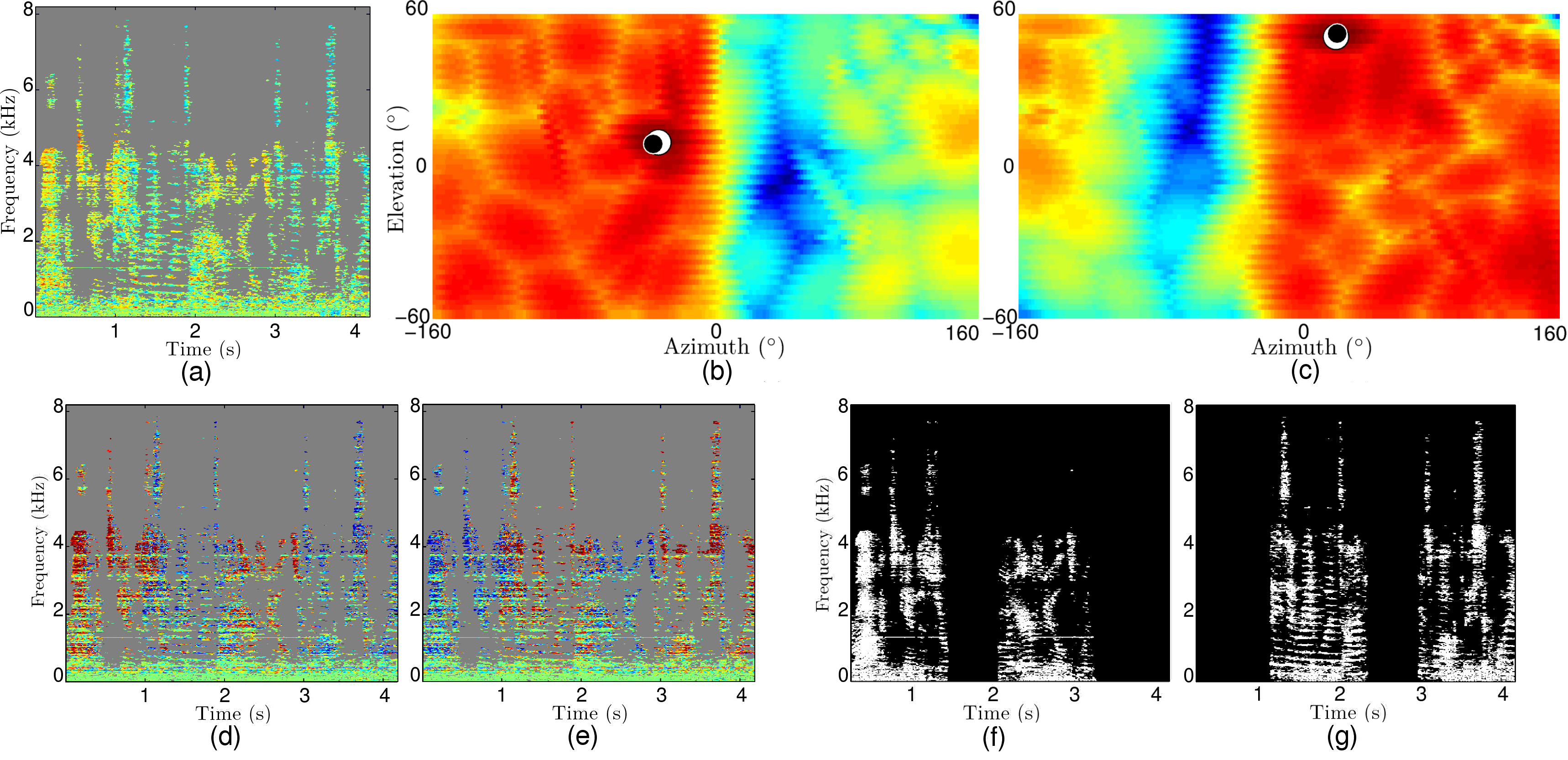
Fig. 7: (a) Input ILD spectrogram. (b,c) Output log-density of each source position as determined by $q^{(\infty)}_{X,Z}$. Ground-truth source positions are noted with a black dot, and the peak of the log-density with a white circle. (d,e) Output source assignment probabilities $q^{(\infty)}_{W}$. (f,g) Ground truth binary masks. Red color denotes high values, blue color low values, and grey colors missing observations.

$$\mbox{\boldmath$\mu$}_{km}^{(i)}=\mbox{\bf S}_{km}^{(i)}\bigg{(}\mbox{\boldmath$\Gamma$}_{k}^{-1}\mbox{\boldmath$c$}_{k}+\textstyle\sum_{d,t}\sigma_{d}^{-2}q_{W_{dt}}^{(i-1)}(m)(y_{dt}-b_{dk})\mbox{\boldmath$a$}_{dk}\bigg{)},\hskip 5.69054pt\mbox{\bf S}_{km}^{(i)}=\bigg{(}\mbox{\boldmath$\Gamma$}_{k}^{-1}+\textstyle\sum_{d,t}\sigma_{d}^{-2}q_{W_{dt}}^{(i-1)}(m)\mbox{\boldmath$a$}_{dk}\mbox{\boldmath$a$}_{dk}^{\top}\bigg{)}^{-1},$$ (19)

$$\alpha_{km}^{(i)}\propto\frac{|\mbox{\bf S}^{(i)}_{km}|^{\frac{1}{2}}}{|\mbox{\boldmath$\Gamma$}_{k}|^{\frac{1}{2}}}\exp\left\{-\frac{1}{2}\left(\textstyle\sum_{d,t}\displaystyle\frac{\chi_{dt}}{\sigma^{2}_{d}}(y_{dt}-\widetilde{b}_{dk})^{2}+\mbox{\boldmath$c$}_{k}^{\top}\mbox{\boldmath$\Gamma$}_{k}^{-1}\mbox{\boldmath$c$}_{k}-\mbox{\boldmath$\mu$}_{km}^{(i)\top}\mbox{\bf S}^{(i)-1}_{km}\mbox{\boldmath$\mu$}_{km}^{(i)}\right)\right\},$$ (20)

$$q_{W_{dt}}^{(i)}(m)\propto\chi_{dt}\lambda^{(i)}_{dm}\prod_{k=1}^{K}\exp\left\{-\frac{\alpha_{km}^{(i)}}{2\sigma_{d}^{2}}\left(\operatorname{tr}(\mbox{\bf S}_{km}^{(i)}\mbox{\boldmath$a$}_{dk}\mbox{\boldmath$a$}_{dk}^{\top})+(y_{dt}-\mbox{\boldmath$a$}_{dk}^{\top}\mbox{\boldmath$\mu$}_{km}^{(i)}-b_{dk})^{2}\right)\right\},$$ (21)

$$\lambda^{(i)}_{dm}=\frac{1}{T}\textstyle\sum_{t}q^{(i)}_{W_{dt}}(m),\;\sigma^{2(i)}_{d}=\displaystyle\frac{\sum_{t,m,k}q_{W_{dt}}^{(i)}(m)\;\alpha_{km}^{(i)}\;\bigl{(}\operatorname{tr}(\mbox{\bf S}_{km}^{(i)}\mbox{\boldmath$a$}_{dk}\mbox{\boldmath$a$}_{dk}^{\top})+(y_{dt}-\mbox{\boldmath$a$}_{dk}^{\top}\mbox{\boldmath$\mu$}_{km}^{(i)}-b_{dk})^{2}\bigr{)}}{\sum_{t,m,k}q_{W_{dt}}^{(i)}(m)\;\alpha_{km}^{(i)}}.$$ (22)

E-XZ step: The update of $q_{X,Z}$ is given by:

$$q_{X,Z}^{(i)}(\mbox{\boldmath$x$},\mbox{\boldmath$z$})\propto\exp\mathbb{E}{q_{W}^{(i-1)}}[\log p(\mbox{\boldmath$x$},\mbox{\boldmath$z$}|\mbox{\boldmath$y$},\mbox{\boldmath$W$};\mbox{\boldmath$\psi$}^{(i)})].$$

It follows from standard algebra that

$$q_{X,Z}^{(i)}(\mbox{\boldmath$x$},\mbox{\boldmath$z$})=\textstyle\prod_{m=1}^{M}\alpha_{km}^{(i)}\mathcal{N}(\mbox{\boldmath$x$};\mbox{\boldmath$\mu$}_{km}^{(i)},\mbox{\bf S}_{km}^{(i)})$$

where $\mbox{\boldmath$\mu$}_{km}^{(i)},\mbox{\bf S}_{km}^{(i)},\alpha_{km}^{(i)}$ are given in (19),(20) and the weights $\{\alpha_{km}^{(i)}\}_{k=1}^{K}$ are normalized to sum to 1 over $k$ for all $m$. One can see this step as the localization step, since it corresponds to estimating a mixture of Gaussians over the latent space $\mathcal{X}$ of positions for each source. When $M=1$, $W$ is entirely determined and $q_{W_{dt}}=\chi_{dt}$. Thus, we can directly obtain the probability density $q_{X,Z}$ of the sound source position using (19),(20), and we recover exactly the single-source formula (13), (14), (5.2).

E-W step: The update of $q_{W}$ is given by:

$$q_{W}^{(i)}(\mbox{\boldmath$w$})\propto\exp\mathbb{E}{q_{X,Z}^{(i)}}[\log p(\mbox{\boldmath$w$}|\mbox{\boldmath$y$},\mbox{\boldmath$X$},\mbox{\boldmath$Z$};\mbox{\boldmath$\psi$}^{(i)})].$$

It follows that $q_{W}^{(i)}(\mbox{\boldmath$w$})=\prod_{d,t}q_{W_{dt}}^{(i)}(w_{dt})$ where $q_{W_{dt}}^{(i)}$ is given in (21) and is normalized to sum to 1 over $m$. This can be seen as the sound source separation step, as it provides the probability of assigning each observation to each source.

M step: We need to solve for:

$$\mbox{\boldmath$\psi$}^{(i+1)}=\operatorname{argmax}_{\mbox{\boldmath$\psi$}}\mathbb{E}q_{W}^{(i)}q_{X,Z}^{(i)}[\log p(\mbox{\boldmath$y$},\mbox{\boldmath$W$},\mbox{\boldmath$X$},\mbox{\boldmath$Z$};\mbox{\boldmath$\psi$})].$$

This reduces to the update of the source weights $\mbox{\boldmath$\Lambda$}^{(i)}$ and noise variances $\mbox{\boldmath$\Sigma$}^{(i)}=\operatorname{diag}(\sigma_{1}^{2(i)}...\sigma_{D}^{2(i)})$ as given by (22).

Method	ILD only		IPD only		ILPD
used	Azimuth	Elevation	Azimuth	Elevation	Azimuth	Elevation
PPAM	2.2$\pm$1.9	1.6$\pm$1.6	1.5$\pm$1.3	1.5$\pm$1.4	1.8 $\pm$1.6	1.6$\pm$1.5
MPLR	2.4$\pm$2.2	2.2$\pm$2.1	1.8$\pm$1.7	1.9$\pm$1.7	2.2 $\pm$2.0	2.1$\pm$2.0
SIR-1	41$\pm$34	17$\pm$13	36$\pm$25	24$\pm$17	41$\pm$34	16$\pm$13
SIR-2	27$\pm$28	14$\pm$13	32$\pm$23	11$\pm$11	26$\pm$28	14$\pm$13

Table 1: Comparing the average and standard deviation (Avg$\pm$Std) of azimuth and elevation angular errors in degrees using different types of interaural vectors obtained from white noise recordings and different mapping techniques.

Initialization strategies: Extensive real world experiments show that the VEM objective function, called the variational free energy, have a large number of local maxima. This may be due to the combinatorial size of the set of all possible binary masks $\mathcal{W}$ and the set of all possible affine transformation assignments $\mathcal{Z}$. Indeed, the procedure turns out to be more sensitive to initialization and to get trapped in suboptimal solutions more often as the size of the spectrogram and the number of transformations $K$ are increased. On the other hand, too few local affine transformations $K$ make the mapping very imprecise. We thus developed a new efficient way to deal with the well established local maxima problem, referred to as multi-scale initialization. The idea is to train PPAM at different scales, i.e., with a different number of transformations $K$ at each scale, yielding different sets of trained parameters $\widetilde{\theta}_{K}$ where, e.g., $K=1,2,4,8\dots,64$. When proceeding with the inverse mapping, we first run the VEM algorithm from a random initialization using $\widetilde{\theta}_{1}$. We then use the obtained masks and positions to initialize a new VEM algorithm using $\widetilde{\theta}_{2}$, then $\widetilde{\theta}_{4}$, and so forth until the desired value for $K$. To further improve the convergence of the algorithm at each scale, an additional constraint is added, namely progressive masking. During the first iteration, the mask of each source is constrained such that all the frequency bins of each time frame are assigned to the same source. This is done by adding a product over $t$ in the expression of $q^{(1)}_{W_{dt}}(m)$ (21). Similarly to what is done in^?, this constraint is then progressively released at each iteration by dividing time frames in $2,4,8\dots,F$ frequency blocks until the total number of frequency bins $F$ is reached. Combining these two strategies dramatically increases both the performance and speed${}^{\mbox{\scriptsize d}}$ of the proposed VESSL algorithm.

Algorithm termination: Maximum a posteriori (MAP) estimates for missing data can be easily obtained at convergence of the algorithm by maximizing respectively the final probability distributions $q^{(\infty)}_{X,Z}(\mbox{\boldmath$x$},\mbox{\boldmath$z$})$ and $q^{(\infty)}_{W}(\mbox{\boldmath$w$})$. We have $(\mbox{\boldmath$X$}_{m}^{MAP},Z_{m}^{MAP})=(\mbox{\boldmath$\mu$}^{(\infty)}_{\hat{k}m},\hat{k})$ where $\hat{k}=\operatorname*{argmax}_{k}\alpha^{(\infty)}_{km}\;|\mbox{\boldmath$\Sigma$}^{(\infty)}_{km}|^{-1/2}$ and $W_{dt}^{MAP}=\operatorname*{argmax}_{m}q^{(\infty)}_{W_{dt}}(m)$. Note that as shown in Fig. 7, the algorithm not only provides MAP estimates, but also complete posterior distributions over both the 2D space of sound source positions $\mathcal{X}$ and the space of source assignments $\mathcal{W}$. Using the final assignment probabilities $q^{(\infty)}_{W_{dt}}(m)$ of source $m$, one can multiply recorded spectrogram values $s_{ft}^{(\textrm{L})}$ and $s_{ft}^{(\textrm{R})}$ by $1$ if $m$ has the highest emission probability at $(f,t)$, and $0$ otherwise (binary masking). This approximates the spectrogram $\{s^{(\textrm{m})}_{ft}\}_{f,t=1}^{F,T}$ emitted by source $m$, from which the original temporal signal can be recovered using inverse Fourier transform, hence achieving sound source separation.

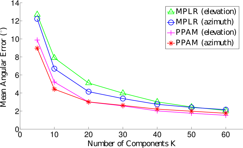
Fig. 8: Comparison of the proposed method (PPAM) with MPLR (Qiao and Minematsu 2009) as a function of the number of components.

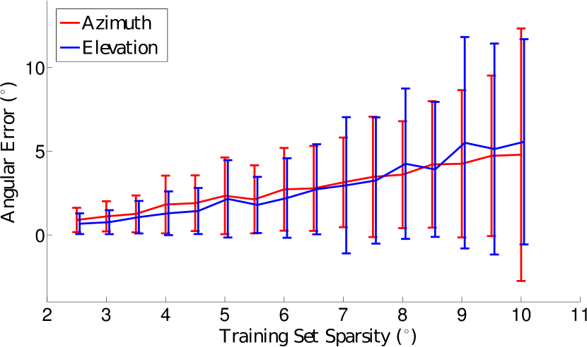
Fig. 9: Average and standard deviation of angular errors in white noise localization as a function of the training set’s sparsity.

7 Results on Acoustic Space Mapping, Source Localization and Sound Separation

We first compare PPAM to two other existing mapping methods, namely mixture of probabilistic linear regression (MPLR^?), and sliced inverse regression (SIR^?). MPLR may be viewed as a unifying view of joint GMM mapping techniques, which consists of estimating a standard Gaussian mixture model on joint variables $[\mbox{\boldmath$X$};\mbox{\boldmath$Y$}]$ and uses conditional expectations to infer the mapping. Joint GMM has been widely used in audio applications^?,?,?,?. SIR quantizes the low-dimensional data $X$ into slices or clusters which in turn induces a quantization of the $Y$-space. Each $Y$-slice (all points $\mbox{\boldmath$y$}_{n}$ that map to the same $X$-slice) is then replaced with its mean and PCA is carried out on these means. The resulting low-dimensional representation is then informed by $X$ values through the preliminary slicing. We selected one (SIR-1) or two (SIR-2) principal axes for dimensionality reduction, 20 slices (the number of slices is known to have little influence on the results), and polynomial regression of order three (higher orders did not show significant improvements). We use $K=64$ for both PPAM and MPLR. All techniques are trained on three types of cues: full spectrum ILD only, low-IPD only and ILPD cues (see Section 2 and 4). For each type of cue, the training is done on $10$ random subsets of $4,800$ mean interaural vectors obtained from white noise recordings emitted by sources spanning a $[-160^{\circ},160^{\circ}]$ azimuth range and $[-60^{\circ},60^{\circ}]$ elevation range (section 3), and tested on the mean interaural vectors of the remaining $4,800$ source positions ($96,000$ tests in total). The resulting angular errors are shown in Table 1. As it may be seen, PPAM always performs best, validating the choice of piecewise-affine probabilistic technique adapted to the manifold structure of interaural data. The poor performance of SIR can be explained by the important non-linear nature of the data. Although pure IPD cues show slightly better localization results than pure ILD cues, it is better to use both to maximize the available information in the case of noisy and/or missing data. Other experiments in this section are therefore carried out using ILPD cues.

Fig. 9 shows the influence of the number of affine components $K$ on PPAM’s and MPLR’s localization results using similar test and training sets. Better performance of PPAM can be explained by the fact that the number of parameters to estimate in joint GMM methods increases quadratically with the dimensionality, and thus becomes prohibitively high using ILPD data ($D=730$). Unsurprisingly, the localization error decreases when $K$ increases. In practice, too high values of $K$ (less than 20 samples per affine component) may lead to some degenerate covariance matrices in components where there are too few samples. Such components are simply removed along the execution of the algorithm, thus reducing $K$. In other words, the only free parameter $K$ of PPAM can be chosen based on a compromise between computational cost and precision.

Method	1 source
used	Az $({}^{\circ})$	El $({}^{\circ})$
PPAM(T1)	$2.1\pm 2.1$	$1.1\pm 1.2$
PPAM(T2)	$3.5\pm 3.3$	$2.4\pm 2.6$
PHAT	$7.6\pm 9.4$

Table 2: Average single sound source localization error in degrees using PHAT and PPAM with two different training sets.

Fig. 9 shows the influence of the training set’s sparsity on PPAM’s localization results. We represent the sparsity by an angle $\delta$, corresponding to the average pan and tilt absolute difference between a point and its nearest neighbor in the training set. The complete training set of sparsity $2^{\circ}$ was uniformly decimated at random to obtain irregularly spaced and smaller training sets, while the test positions were randomly chosen from the remaining ones. For a given sparsity $\delta$, 10 different decimated sets were used for training, and 100 source positions were estimated for each one, i.e., 1000 localization tasks. $K$ was chosen to have approximately 30 training samples per affine component. The mean and standard deviation of the errors in azimuth and in elevation are shown in Fig. 9. The mean localization errors are always smaller than half the training set sparsity, which illustrates the interpolation ability of our method. In addition, the error’s standard deviation remains reasonable even for heavily decimated training sets ($384$ points only for $\delta=10^{\circ}$), thus showing that the overall performance is not much affected by the distribution and size of the training set being used. With the automatic audio-motor technique described in Section 3, recording a training set of sparsity $2^{\circ}$ ($9,600$ points) requires 2 hours and 30 minutes while it takes 25 minutes with a sparsity of $5^{\circ}$ ($1,530$ points).

Method	2 sources				3 sources
used	Az	El	SDR	STIR	Az	El	SDR	STIR
VESSL(T1)	4.7$\pm$11	2.9$\pm$9.9	3.8$\pm$1.7	6.1$\pm$1.7	12 $\pm$21	8.7$\pm$19	1.7$\pm$1.5	2.2$\pm$1.5
VESSL(T2)	8.2$\pm$16	4.7$\pm$11	3.3$\pm$1.6	5.2$\pm$1.6	16 $\pm$24	9.1$\pm$18	1.5$\pm$1.5	1.8$\pm$1.5
MESSL-G	14$\pm$21		2.3$\pm$1.6	6.0$\pm$4.3	18$\pm$28		1.3$\pm$1.2	2.1$\pm$4.4
mixture			0.0$\pm$2.5	0.2$\pm$2.5			-3.2$\pm$2.3	-3.0$\pm$2.3
oracle			12$\pm$ 1.6	21 $\pm$2.0			11$\pm$ 1.7	20 $\pm$2.1

Table 3: Comparing the average and standard deviation (Avg$\pm$Std) of azimuth (Az) and elevation (El) angular errors in degrees, as well as Signal to Distortion Ratio (SDR) and Signal to Inteferer Ratio (STIR) for 600 test mixtures of 2 to 3 sources using different methods.

We also tested the ability of PPAM to localize a single sound source using real world recordings of randomly located sources emitting random utterances (see Section 3), using the technique presented in Section 5.2. We use both the complete set of ILPD cues T1 (sparsity $\delta=2^{\circ}$) and a partial set T2 of sparsity $\delta=5^{\circ}$ for training. We set $K=128$ for T1 and $K=64$ for T2. Test sounds are chosen to be outside of the training set T2. The spectral power threshold is manually set quite high, so that test spectrograms has $89.6\%$ of missing data, on average. Results are compared to a baseline sound localization method, namely PHAT-histogram^?. As the vast majority of existing source localization methods^?,?,?,?,?,?, PHAT-histogram provides a time difference of arrival (TDOA) which can only be used to estimate frontal azimuth. The link between TDOAs and azimuths is estimated using linear regression on our dataset. For the comparison to be fair, PHAT is only tested on frontal sources. Comparison with the few existing binaural 2D sound source localization methods^?,? is not possible because they rely on additional knowledge of the system being used that are not available. Means and standard deviations of azimuth (Az) and elevation (El) errors (Avg$\pm$Std) are shown in Table 2.

The proposed acoustic space learning approach dramatically outperforms the baseline. No front-back azimuth or elevation confusions is observed using our method, thanks to the asymmetry of the dummy head and to the spatial richness of interaural spectral cues.

We finally tested the ability of VESSL (section 6) to localize and separate multiple sound sources emitting at the same time. We use both training sets T1 and T2 for training and mixtures of 2 to 3 sources for testing${}^{\mbox{\scriptsize e}}$. Mixtures are obtained by summing binaural recordings of sources emitting random utterances from random positions (see Section 3) so that at least two sources were emitting at the same time in $60\%$ of the test sounds. Localization and separation results are compared to state-of-the-art EM-based sound source separation and localization algorithm MESSL^?. MESSL does not rely on acoustic space learning, and estimates a time difference of arrival for each source. As for PHAT-histogram, results given for MESSL correspond to tests with frontal sources only. The version MESSL-G that is used includes a garbage component and ILD priors to better account for reverberations and is reported to outperform four methods in reverberant conditions in terms of separation^?,?,?,?. We evaluate separation performance using the standard metrics signal to distortion ratio (SDR) and signal to interferer ratio (STIR) introduced in^?. SDR and STIR scores of both methods are also compared to those obtained with the ground truth binary masks or oracle masks^? and to those of the original mixture. Oracle masks provide an upper bound for binary masking methods that cannot be reached in practice because it requires knowledge of the original signals. Conversely, the mixture scores provide a lower bound, as no mask is applied. Table 3 shows that VESSL significantly outperforms MESSL-G both in terms of separation and localization, putting forward acoustic space learning as a promising tool for accurate sound source localization and separation.

8 Conclusion and Future Work

We showed the existence of binaural manifolds, i.e. an intrinsic locally-linear, low-dimensional structure hidden behind the complexity of interaural data obtained from real world recordings. Based on this key property, we developed a probabilistic framework to learn a mapping from sound source positions to interaural cues. We showed how this framework could be used to accurately localize in both azimuth and elevation and separate mixtures of natural sound sources. Results show the superiority of acoustic space learning compared to other sound source localization techniques relying on simplified mapping models.

In this work, auditory data are mapped to the motor-states of a robotic system, but the same framework could be exploited with mappings of different nature. Typically, for unsupervised sound source localization where one only has access to non-annotated auditory data from different locations, one may map auditory cues to their intrinsic coordinates obtained using manifold learning, as explained in Section 4. Such coordinates are spatially consistent, i.e., two sources that are near will yield near coordinates, but are not linked to a physical quantity and may therefore be hard to interpret or evaluate. Alternatively, auditory data could be annotated with the pixel position of the sound source in an image, yielding audio-visual mapping instead of audio-motor mapping.

A direction for future work is to study the influence of changes in the reverberating properties of the room where the training is performed. The PPAM model could be extended by adding latent components modeling such changes^?, thus becoming more robust to the recording environment. Another open problem is determining the number of sound sources $M$ in the mixture, which is generally challenging in source separation. In our framework, it corresponds to a model selection problem, which could be addressed using, e.g., a Bayesian information theoretic analysis.

References

References

- [1] J. Blauert, Spatial Hearing: The Psychophysics of Human Sound Localization, MIT Press, (1997).
- [2] D. Wang and G. J. Brown, Computational Auditory Scene Analysis: Principles, Algorithms and Applications, IEEE Press, (2006).
- [3] A. Deleforge and R. P. Horaud, “The cocktail party robot: Sound source separation and localisation with an active binaural head,” In ACM/IEEE International Conference on Human Robot Interaction, 431–438, (2012).
- [4] E. C. Cherry, “Some experiment on the recognition of speech, with one and with two ears,” The Journal of the Acoustical Society of America, 25(5), 975–979, September (1953).
- [5] S. Haykin and Z. Chen, “The cocktail party problem,” Neural Computation, 17, 1875–1902, (2005).
- [6] L. Rayleigh, “On our perception of sound direction,” Philos. Mag., 13, 214–232, April (1907).
- [7] J. C. Middlebrooks and D. M. Green, “Sound localization by human listeners,” Annual Review of Psychology, 42, 135–159, (1991).
- [8] R. S. Woodworth and H. Schlosberg, Experimental Psychology, Holt, (1965).
- [9] P. M. Hofman and A. J. Van Opstal, “Spectro-temporal factors in two-dimensional human sound localization,” The Journal of the Acoustical Society of America, 103(5), 2634–2648, (1998).
- [10] R. Liu and Y. Wang, “Azimuthal source localization using interaural coherence in a robotic dog: modeling and application,” Robotica, 28(7), 1013–1020, (2010).
- [11] X. Alameda-Pineda and R. P. Horaud, “Geometrically constrained robust time delay estimation using non-coplanar microphone arrays,” In European Signal Processing Conference, 1309–1313, (2012).
- [12] M. I. Mandel, D. P. W. Ellis, and T. Jebara, “An EM algorithm for localizing multiple sound sources in reverberant environments,” In Neural Information Processing Systems, 953–960, (2007).
- [13] A. Deleforge and R. P. Horaud, “A latently constrained mixture model for audio source separation and localization,” In The Tenth International Conference on Latent Variable Analysis and Signal Separation, 372–379, (2012).
- [14] J. Woodruff and D. Wang, “Binaural localization of multiple sources in reverberant and noisy environments,” IEEE Transactions on Acoustics, Speech, Signal Processing, 20(5), 1503–1512, (2012).
- [15] O. Yılmaz and S. Rickard, “Blind separation of speech mixtures via time-frequency masking,” IEEE Transactions on Signal Processing, 52, 1830–1847, (2004).
- [16] H. Viste and G. Evangelista, “On the use of spatial cues to improve binaural source separation,” In International Conference on Digital Audio Effects, 209–213, (2003).
- [17] A. R. Kullaib, M. Al-Mualla, and D. Vernon, “2d binaural sound localization: for urban search and rescue robotics,” In Mobile Robotics, 423–435, (2009).
- [18] F. Keyrouz, W. Maier, and K. Diepold, “Robotic localization and separation of concurrent sound sources using self-splitting competitive learning,” In IEEE Symposium on Computational Intelligence in Image and Signal Processing, 340–345, (2007).
- [19] J. Hörnstein, M. Lopes, J. Santos-Victor, and F. Lacerda, “Sound localization for humanoid robots – building audio-motor maps based on the HRTF,” In IEEE/RSJ International Conference on Intelligent Robots and Systems, 1170–1176, (2006).
- [20] P. M. Hofman, J. G. Van Riswick, A. J. Van Opstal, et al., “Relearning sound localization with new ears,” Nature neuroscience, 1(5), 417–421, (1998).
- [21] B. A. Wright and Y. Zhang, “A review of learning with normal and altered sound-localization cues in human adults,” International journal of audiology, 45(S1), 92–98, (2006).
- [22] M. Aytekin, C. F. Moss, and J. Z. Simon, “A sensorimotor approach to sound localization,” Neural Computation, 20(3), 603–635, (2008).
- [23] H. Poincaré, The foundations of science; Science and hypothesis, the value of science, science and method, New York: Science Press, (1929), Halsted, G. B. trans. of La valeur de la science, 1905.
- [24] J. K. O’Regan and A. Noe, “A sensorimotor account of vision and visual consciousness,” Behavioral and Brain Sciences, 24, 939–1031, (2001).
- [25] R. Held and A. Hein, “Movement-produced stimulation in the development of visually guided behavior,” J. Comp. Physiol. Psych., 56(5), 872–876, (1963).
- [26] A. Deleforge and R. P. Horaud, “2d sound-source localization on the binaural manifold,” In IEEE Workshop on Machine Learning for Signal Processing, 1–6, (2012).
- [27] A. Deleforge, F. Forbes, and R. P. Horaud, “Variational em for binaural sound-source separation and localization,” In IEEE International Conference on Acoustics, Speech, and Signal Processing, 76–80 (, Vancouver, Canada, 2013).
- [28] S. T. Roweis, “One microphone source separation,” In Advances in Neural Information Processing Systems, volume 13, 793–799. MIT Press, (2000).
- [29] S. Bensaid, A. Schutz, and D. T. M. Slock, “Single microphone blind audio source separation using EM-Kalman filter and short+long term AR modeling,” In Latent Variable Analysis and Signal Separation, 106–113, (2010).
- [30] P. Comon and C. Jutten, Handbook of Blind Source Separation, Independent Component Analysis and Applications, Academic Press (Elsevier), (2010).
- [31] N.Q.K. Duong, E. Vincent, and R. Gribonval, “Under-determined reverberant audio source separation using a full-rank spatial covariance model,” IEEE Transactions on Audio Signal and Langage Processing, 18(7), 1830–1840, (2010).
- [32] M. I. Mandel, R. J. Weiss, and D. P. W. Ellis, “Model-based expectation-maximization source separation and localization,” IEEE Transactions on Audio, Speech and Language Processing, 18(2), 382–394, (2010).
- [33] R. Rosipal and N. Krämer, “Overview and recent advances in partial least squares,” Subspace, Latent Structure and Feature Selection, 3940, 34–51, (2006).
- [34] K. C. Li, “Sliced inverse regression for dimension reduction,” The Journal of the American Statistical Association, 86(414), 316–327, (1991).
- [35] H. M. Wu, “Kernel sliced inverse regression with applications to classification,” Journal of Computational and Graphical Statistics, 17(3), 590–610, (2008).
- [36] R. D. de Veaux, “Mixtures of linear regressions,” Computational Statistics and Data Analysis, 8(3), 227–245, (1989).
- [37] L. Xu, M. I. Jordan, and G. E. Hinton, “An alternative model for mixtures of experts,” In Proc. of the Neural Information Processing Systems (NIPS) conference, volume 7, 633–640, (1995).
- [38] A. Kain and MW Macon, “Spectral voice conversion for text-to-speech synthesis,” In IEEE International Conference on Acoustics, Speech, and Signal Processing, volume 1, 285–288, (1998).
- [39] Y. Stylianou, O. Cappé, and E. Moulines, “Continuous probabilistic transform for voice conversion,” IEEE Transactions on Acoustics, Speech, Signal Processing, 6, 131–142, (1998).
- [40] T. Toda, A. Black, and K. Tokuda, “Statistical mapping between articulatory movements and acoustic spectrum using a gaussian mixture model,” Speech Communication, 50(3), 215–227, (2008).
- [41] Y. Qiao and N. Minematsu, “Mixture of probabilistic linear regressions: A unified view of GMM-based mapping techniques,” In IEEE International Conference on Acoustics, Speech, and Signal Processing, 3913–3916, (2009).
- [42] A. Deleforge, F. Forbes, and R. P. Horaud, “High-dimensional regression with gaussian mixtures and partially-latent response variables, arxiv:1308.2302, December (2013).
- [43] M. Otani, T. Hirahara, and S. Ise, “Numerical study on source-distance dependency of head-related transfer functions,” The Journal of the Acoustical Society of America, 125(5), 3253–61, (2009).
- [44] J. S. Garofolo, L. F. Lamel, and W. M. Fisher, “The darpa timit acoustic-phonetic continuous speech corpus cdrom”, (1993).
- [45] R. Talmon, I. Cohen, and S. Gannot, “Supervised source localization using diffusion kernels,” In IEEE Workshop on Applications of Signal Processing to Audio and Acoustics, 245 –248 (, New Paltz, New York, 2011).
- [46] Zhenyue Zhang and Hongyuan Zha, “Principal manifolds and nonlinear dimensionality reduction via tangent space alignment,” SIAM Journal on Scientific Computing, 26(1), 313–338, (2005).
- [47] M. Beal and Z. Ghahramani, “The variational Bayesian EM algorithm for incomplete data: with application to scoring graphical model structures,” Bayesian Statistics, 7, 453–464, (2003).
- [48] P. Aarabi, “Self-localizing dynamic microphone arrays,” IEEE Transactions on Systems, Man, and Cybernetics, Part C: Applications and Reviews, 32(4), 474–484, (2002).
- [49] J. Mouba and S. Marchand, “A source localization/separation/respatialization system based on unsupervised classification of interaural cues,” In International Conference on Digital Audio Effects, 233–238 (, Montreal, Canada, 2006).
- [50] H. Buchner, R. Aichner, and W. Kellermann, “A generalization of blind source separation algorithms for convolutive mixtures based on second-order statistics,” IEEE Transactions on Audio, Speech and Language Processing, 13(1), 120–134, (2005).
- [51] H. Sawada, S. Araki, and S. Makino, “A Two-Stage Frequency-Domain Blind Source Separation Method for Underdetermined Convolutive Mixtures,” In IEEE Workshop on Applications of Signal Processing to Audio and Acoustics, 139–142 (, New Paltz, New York, 2007).
- [52] E. Vincent, R. Gribonval, and C. Févotte, “Performance measurement in blind audio source separation,” IEEE Transactions on Audio, Speech and Language Processing, 14(4), 1462–1469, (2006).