SMA millimeter observations of Hot Molecular Cores

Abstract

We present Submillimeter Array observations, in the 1.3 mm continuum and the CH₃CN (12_K–11_K)  line of 17 hot molecular cores associated with young high-mass stars. The angular resolution of the observations ranges from 1$\farcs$0 to 4$\farcs$0. The continuum observations reveal large ($>$3500 AU) dusty structures with gas masses from 7 to 375 M_⊙, that probably surround multiple young stars. The CH₃CN line emission is detected toward all the molecular cores at least up to the $K=6$-component and is mostly associated with the emission peaks of the dusty objects. We used the multiple $K$-components of the CH₃CN  and both the rotational diagram method and a simultaneous synthetic LTE model with the XCLASS program to estimate the temperatures and column densities of the cores. For all sources, we obtained reasonable fits from XCLASS by using a model that combines two components: an extended and warm envelope, and a compact hot core of molecular gas, suggesting internal heating by recently formed massive stars. The rotational temperatures lie in the range of 40-132 K and 122-485 K for the extended and compact components, respectively. From the continuum and CH₃CN results, we infer fractional abundances from $10^{-9}$ to $10^{-7}$ toward the compact inner components, that increase with the rotational temperature. Our results agree with a chemical scenario in which the CH₃CN molecule is efficiently formed in the gas phase above 100-300 K, and its abundance increases with temperature.

1. INTRODUCTION

Massive stars ($M>8$ $M_{\odot}$) are born inside of dense cores located in large and massive molecular clouds (e.g., Garay & Lizano, 1999; Cesaroni, 2005). These massive star-forming regions (MSFRs) have a substantial impact on the evolution of the interstellar medium (ISM) and make important contributions to its dynamics and chemistry. For example, molecular outflows, jets, stellar winds and supernovae associated with MSFRs push into their surroundings, promoting additional star formation and mixing the ISM.

One of the first manifestations of massive star formation is the so-called hot molecular core phase (HMCs; Kurtz et al., 2000; Cesaroni, 2005). This phase is characterized by molecular gas condensations at relatively high temperatures ($>$100 K) and high densities ($\sim$10⁵–10⁸ cm^-3), associated with a compact ($<$ 0.1 pc), luminous ($>$ 10⁴ $L_{\odot}$), and massive ($\sim$10-1000 $M_{\odot}$) molecular core.

HMCs show a forest of molecular lines, especially from organic species (e.g., Comito et al., 2005). Many of these molecules probably were formed on grain mantles during a previous cold phase, while others were produced by gas-phase reactions after “parents species” were evaporated from the grains by the strong radiation of embedded or nearby protostars (see Herbst & van Dishoeck, 2009).

Both models and observations suggest that massive HMCs are collapsing and accreting mass onto a central source(s) at rates of $10^{-4}-10^{-3}$ $M_{\odot}$ yr^-1 (Osorio et al., 2009; Zapata et al., 2009). These intense mass accretion rates are high enough to prevent the development of an ionized region around the massive star(s) at least in the early stages (Osorio et al., 1999). Thus, HMCs probably precede ultracompact HII regions (UC HII; Kurtz et al., 2000; Wilner et al., 2001). Indeed, sub-arcsecond observations argue in favor of this scenario, particularly those showing embedded UC HII-regions, strong (sub)millimeter emission from dust condensations, or strong mid-IR emission from internal objects (e.g.; Cesaroni et al., 2010, 2011).

In the above scenario a HMC corresponds to the most internal clump of molecular material collapsing and probably feeding other structures and the massive stars inside (Cesaroni, 2005; Wilner et al., 2001). However, recent sensitive high angular resolution observations suggest that the prototypical HMC, Orion BN/KL, may not follow this model. In this case, a close dynamical interaction of three young protostars produced an explosive flow and illuminated a pre-existing dense clump, thus creating the HMC (Zapata et al., 2011; Goddi et al., 2011). Also, toward G34.26+0.15 (another prototypical HMC), Mookerjea et al. (2007) failed to find any embedded protostars within the hot core. The different nature of internally and externally heated HMC makes it important to distinguish between them.

With this in mind, we present a study using Submillimeter Array (SMA) archival observations of CH₃CN (12_K–11_K) and 1.3 mm continuum emission, toward 17 MSFRs in the HMC stage. CH₃CN (methyl cyanide) is frequently used as an effective thermometer and to estimate gas density toward HMCs (e.g., Araya et al., 2005a; Pankonin et al., 2001). Our main goal is to use the same molecular tracer toward a relatively large group of sources to study the inner-most and hottest material, estimating densities, temperatures, masses, abundances, and the spatial distribution of the dust emission and CH₃CN molecular gas.

In Section 2 we describe the archival observations presented in this study. In Section 3 we report the results and analysis of the millimeter continuum data and the molecular line emission. In Section 4 we comment briefly on each source, giving the physical characteristics from the literature and from our results. In Section 5 we discuss our results, first comparing the spatial distribution of the continuum emission and molecular emission, and then estimating the temperatures and densities of the regions from an LTE analysis of the CH₃CN (12_K–11_K)  spectra and through the rotation diagram method. Finally, in Section 6, we present our main conclusions.

2. OBSERVATIONS AND DATA REDUCTION

We searched the literature for MSFRs in the HMC phase, based on previous detection of molecular species indicating warm and dense gas such as CH₃CN, NH₃ and CH₃OH. These molecules are commonly used to trace HMCs (e.g., Churchwell et al., 1990, 1992; Olmi et al., 1993; Kalenskii et al., 1997, 2000). We compiled a list of almost 60 objects of which most are associated with UC HII regions, strong (sub)millimeter emission, molecular outflows, or maser emission; i.e., they are young MSFRs. Then we searched in the SMA archive for observations that included the CH₃CN (12_K–11_K) transitions at $\sim$220.7 GHz. Of the nearly 60 objects, 17 were previously observed in the compact or extended configurations and their data are public.

In Table SMA millimeter observations of Hot Molecular Cores we list the observed sources, their coordinates, lsr velocities, distances, and luminosities, and indicate whether a UC HII region is present. If the 1.3 mm continuum or CH₃CN (12_K–11_K) data were previously published, we list the paper in Table SMA millimeter observations of Hot Molecular Cores. Distances range from 1 to 8.5 kpc, with a mean of 5.0 kpc. Luminosities were in most cases estimated from IRAS fluxes and range from 10⁴ to some 10⁵ $L_{\odot}$. Twelve of the MSFRs (70%) host UC HII regions.

The HMCs were observed with the SMA (Ho et al., 2004) in the compact and/or extended configuration at epochs from April 2004 to April 2010. The maximum projected baselines of the visibility data ranged from $\sim$53 to $\sim$174 k$\lambda$, with different numbers of antennas at different epochs. The SMA correlator was operated with the double-sideband receiver covering 2 GHz in both the lower and upper sidebands. For G23.01 a single receiver with 4 GHz bandwidth was used. The lower-sideband (LSB) covered the frequencies of the CH₃CN (12_K–11_K) $K$-components, which range from 220.74726 GHz ($K=0$) to 220.2350 GHz ($K=11$), with uniform spectral resolution of 0.406 MHz ($\sim$0.53 km s^-1) or 0.812 MHz ($\sim$1.1 km s^-1) for different sources (see Table SMA millimeter observations of Hot Molecular Cores). The primary beam of the SMA at 220 GHz has FWHM $\sim$ 55$\farcs$

The gain, flux, and bandpass calibrators used at each epoch are listed in Table SMA millimeter observations of Hot Molecular Cores. Based on the SMA monitoring of quasars, we estimate the uncertainty in the fluxes to be between 15% and 20%. The visibilities from each observation were calibrated with the IDL-based MIR package (adapted for the SMA), and were then exported to MIRIAD for further processing. The 1.3 mm continuum emission was derived from the line-free channels of the LSB in the visibility domain. All the line data were smoothed to a spectral resolution of 0.812 MHz or $\sim$1.1 km s^-1to improve the sensitivity and provide uniform spectra. The synthesized beam sizes range from 1$\farcs$47$\times$0$\farcs$83 to 5$\farcs$34$\times$2$\farcs$95. In Table SMA millimeter observations of Hot Molecular Cores we summarize the relevant information concerning the observations.

3. RESULTS AND ANALYSIS

3.1. Millimeter continuum data

In Figures 1 to 3 we show the 1.3 mm continuum emission images overlaid with three $K$-lines ($K=3$, 5 and 7) of CH₃CN (12_K–11_K) emission toward the 17 HMCs. Table 3 shows the corresponding continuum emission parameters, derived using line-free channels from the LSB. Using the task imfit in MIRIAD, we found the position of the peak, and the peak and integrated flux densities. The deconvolved source sizes were determined from two dimensional Gaussian fits.

Since HMCs are chemically rich, the continuum emission may be contaminated by some molecular lines, particularly for extremely rich sources such as I17233, G10.62, G31.41, W51e2 and W51e8. Although we were careful to avoid any obvious contamination during the reduction process, we consider the peak and integrated fluxes as upper limits.

Some HMCs show embedded or very nearby UC HII regions and the 1.3 mm continuum emission may have contributions from both ionized gas emission and from the dust. To estimate the free-free contribution at 1.3 mm we extrapolated the emission between 10 and 45 GHz reported in the literature, assuming optically thin emission, i.e., considering $S_{\nu}\propto\nu^{-0.1}$. For G45.07, G45.47, and W51e2 we choose $\sim$100 GHz for extrapolation of the free-free emission due to their high turnover frequencies. In this way we derived the dust continuum emission for the HMCs which ranges from 0.31 Jy for I18566 to 5.88 Jy for I17233. The measured fluxes and the contribution from thermal dust are presented in Table 3.

To estimate the gas mass and average column density we follow Hildebrand (1983). Assuming optically thin dust emission and a constant gas-to-dust ratio, the gas mass is:

$$M_{\rm gas}=\frac{S_{\rm\nu}D^{2}R_{\rm d}}{B_{\rm\nu}(T_{\rm d})\kappa_{\rm\nu}}$$ (1)

where $S_{\rm\nu}$, $D$, $R_{\rm d}$, $\kappa_{\rm\nu}$ and $B_{\rm\nu}(T_{\rm d})$ are the flux density, distance to the core, gas-to-dust ratio, the dust opacity per unit dust mass, and the Planck function at the dust temperature ($T_{\rm d}$), respectively. Note that $\kappa_{\rm\nu}$ ranges from 0.2 to 3.0 at 1.3 mm, depending on its scaled value with frequency as $\nu^{\rm\beta}$, where $\rm\beta$ is the dust emissivity index (e.g., Hunter et al., 2000; Henning et al., 1995). Following Ossenkopf & Henning (1994) and using $\rm\beta$=1.5, we obtain $\kappa_{1.3\,mm}=0.74$ cm² g^-1, corresponding to a median grain size $a=0.1~{}\mu$m and a grain mass density $\rho_{\rm d}=3$ g cm^-3. Our value of $\kappa_{\nu}$ is very similar to other estimates toward HMCs (e.g., Hunter et al., 1999; Osorio et al., 2009).

In the Rayleigh-Jeans approximation, equation 1 gives

$$\left[\frac{M_{\rm gas}}{\rm M_{\odot}}\right]=432.0\left[\frac{S_{\nu}}{\rm Jy}\right]\left[\frac{D}{\rm kpc}\right]^{2}\left[\frac{T}{\rm K}\right]^{-1}$$ (2)

$$\left[\frac{N_{\rm H_{2}}}{\rm cm^{-2}}\right]=\frac{2.35\times 10^{16}}{\theta^{2}}\left[\frac{S_{\nu}}{\rm Jy}\right]\left[\frac{T}{\rm K}\right]^{-1}$$ (3)

where $\theta$ is the source size in radians and we used the common gas-to-dust ratio of 100. At the high densities of HMCs, dust and gas are probably well-coupled through collisions and we can assume that they are in thermal equilibrium (Kaufman et al., 1998). Thus, we used the high temperatures derived from the CH₃CN (see Section 3.3) to obtain $M_{\rm gas}$  and $N_{\rm H_{2}}$ . These values, obtained from the estimated 1.3 mm dust emission, are presented in Table 3.

We caution that the calculated values for the mass and column density are sensitive to both the dust emissivity index and the temperature assumed for each region. For example, decreasing $\beta$ to 1.0 (while keeping the same temperature) lowers the results by a factor of $\sim$3.3. Also, we note that distance uncertainties may be significant for some sources. For other sources (i.e., W3OH/TW, G5.89, G10.47, G10.62, I18182, G23.01, G45.07, and the W51 region) trigonometric parallaxes have been measured (Reid et al., 2009, 2014); these distances are more accurate.

3.2. Molecular line emission

We detected many molecular lines toward the 17 HMCs, but the strength of each species and transition detected varies from source to source. We used the SPLATALOGUE website to identify by eye the main lines in the LSB spectra which are mostly dominated by species such as ¹³CO and C¹⁸O, plus CH₃CN. Other species frequently detected were SO, SO₂, H${}_{2}^{13}$CO, CS and HNCO.

In Figures 5 and 6 we show the spectrum for each source, obtained from the integrated emission over the region of gas traced by the $K=3$ line, which is very similar to the extended component employed in the XCLASS program (see Section 3.3). We detected $K$-components in all seventeen sources at least up to the $K=5$ line, which traces gas at $\sim$247 K. For six sources, I17233, G10.47, G10.62, G31.41, W51e2, and W51e8 we detected $K=8$ lines with $E_{\rm u}=525$ K (See Table 4). The $K=9$ line is blended with the ¹³CO(2–1) line at $\sim$220.4 GHz, making its detection ambiguous.

A complete line identification and chemical analysis is beyond the scope of this work. Nevertheless, we note that there is substantial chemical differentiation in some sources, including pairs of objects as closely spaced as W3TW-W3OH or W51e2-W51e8. These differences have been explained as due to different physical conditions in each region, different chemical composition of ice-mantles on dust grains or different ages of HMCs (e.g., Herbst & van Dishoeck, 2009).

In Table 4 we present the results from the fit of Gaussian profiles to each CH₃CN $K$-component detected. We used the CLASS software package to estimate the line width ($\Delta$V), the integrated intensity ($\int Tdv$), and the LSR velocity ($V_{\rm LSR}$) for each line. We show in Table 4 the average $K$-component values for $\Delta$V and $V_{\rm LSR}$ toward each HMC.

3.3. Temperature and density of the CH₃CN gas

CH₃CN is considered to be a good tracer of warm–hot and high density gas (e.g., Araya et al., 2005a). Its symmetric-top molecular structure works as a rotor, emitting in multiple $K$-levels within a specific $J$ transition, all within a narrow bandwidth ($\sim$ 0.2 GHz). This spectral characteristic is very useful in order to avoid certain systematic errors that occur when comparing lines of very different frequencies. The $K$-levels are radiatively decoupled, and are populated only through collisions (Solomon et al., 1971), thus the rotational temperature of CH₃CN is close to the kinetic temperature of the gas.

If we assume local thermodynamic equilibrium (LTE) and optically thin gas, CH₃CN is an excellent tracer of kinetic temperature using methods such as rotation diagrams (RDs; Linke et al., 1979; Turner, 1991), population diagrams (PDs; Goldsmith & Langer, 1999; Araya et al., 2005a), and simultaneous fitting of multiple lines in a spectrum (Comito et al., 2005; Schilke et al., 1999). In general, no background radiation is considered, and in the RD and PD methods, uniform temperature and density are assumed.

Following the procedure outlined in Turner (1991) and Araya et al. (2005a) one obtains the linear equation ln$(N_{\rm u}/g_{\rm u})$= ln$(N_{\rm tot}/Q_{\rm rot})-E_{\rm u}/kT_{\rm rot}$, in which the slope is ($-1/T_{\rm rot}$) and ln$(N_{\rm tot}/Q_{\rm rot})$ the intercept. The left-hand side of this equation contains the column density per statistical weight of the molecular energy levels and represents the integrated intensity per statistical weight. In this way, plotting the natural logarithm of $N_{\rm u}/g_{\rm u}$ versus $E_{\rm u}/k$ of each $K$-level of CH₃CN and calculating the best linear fit, $T_{\rm rot}$ and $N_{\rm tot}$ can be inferred. In thermodynamic equilibrium the rotational temperature closely approximates the kinematic temperature of the gas.

As a first approximation we estimated the column density and rotational temperature by means of the RD method. The rotation diagrams are shown in Figure 4 and the results of the linear fits are listed in Table 5. The error bars come from the integrated intensity errors in the fitting to each $K$-transition with CLASS and are shown in Table 4.

In the case of mildly optically thick lines, RDs underestimate the upper level column density and overestimate the rotational temperatures. To first order, problems in these estimations can be overcome using the PD method which accounts for optical depth and the source filling factor as proposed in Goldsmith & Langer (1999). Finally, in the RDs method we assumed one region with a single temperature $T_{\rm rot}$.

A more sophisticated approach is to simultaneously fit multiple lines as outlined by Comito et al. (2005) and Schilke et al. (1999). Their XCLASS program generates a synthetic spectrum for multiple molecular species, assuming multiple emission regions, all assumed to be in LTE. Also, XCLASS accounts for line blends and optical depth. For each emission region the program requires inputs for the source size, column density, rotation temperature, line width, and velocity offset from the $V_{\rm LSR}$. XCLASS uses the CDMS and JPL spectral line database (Pickett et al., 1998; Müller et al., 2005, 2001) for line identification. (See Comito et al., 2005, for details of the procedure).

To form the synthetic spectra we model each source as two distinct emission regions: one extended and warm, with relatively low density, and the other compact and hot, with high density. The size of the regions is degenerate with temperature and column density, depending on the optical depth (See Eq. 6 and 7 of Comito et al., 2005). To avoid this degeneracy, the size of the extended component was fixed and we varied the compact component size from 0.5 to 0.25 the size of the extended component. We fixed the offset from $V_{\rm LSR}$ as estimated directly from the observed spectrum (Table 4).

We probed the parameter space with temperatures between 100 K and 500 K for the compact component, and from 50 K to 150 K for the extended component. For the column density we probed 10¹⁴–10¹⁸ cm^-2 for the compact component, and 10¹²–10¹⁵ cm^-2 for the extended component. The best fit of the synthetic to the observed spectrum was determined by a $\chi^{2}$ analysis. As we approached a better fit we used step sizes of 1 K in temperature and $1\times 10^{12}$ cm^-2 in column density. For $\Delta V$ we probed steps of $\pm$2, $\pm$1 and 0 km s^-1 from a near value to the observed average (Table 4). Most of the sources showed a better fit when we used larger line widths for the compact component than for the extended one. In order to estimate errors, we modeled new synthetic spectra perturbing separately temperatures and column densities until we measured an under/overestimation in 20% of the brightness temperature for the $K=2$ transition (20% is the estimated upper limit flux uncertainty of observations), since such a line is mostly optically thin and not blended by other lines.

In Table 5 we present the final fit values and in Figures 5 and 6 we show the observed and synthetic spectra, respectively. All HMCs showed reasonable fits with observations using the two-component model.

3.4. Virial Masses

Virial mass, $M_{\rm vir}$, can be estimated using the line width and source size. Assuming a power-law density distribution with index $p=1.5$ in a spherical core, we use the expression $M_{\rm vir}=0.40~{}d~{}\theta_{\rm CH_{3}CN}~{}\Delta V^{2}$, where $d$ is the distance, $\theta_{\rm CH_{3}CN}$ is the angular diameter and $\Delta V$ the line width, in kpc, arcsecond, and km s^-1, respectively (See Eq. 1 of Beltrán et al., 2004; MacLaren et al., 1988). This is the central mass assuming that the core has gravitationally bound motion. For $\Delta V$ we used the average line width from the observed spectrum (Column 3 in Table 4), and for the source size we used the extended component from the XCLASS analysis (Table 5).

In the last column of Table 5 we present the calculated $M_{\rm vir}$, which ranges from 60 to 473 $M_{\odot}$, with a median of 209 $M_{\odot}$. We note that most of the $M_{\rm vir}$ values are greater than $M_{\rm gas}$. This imbalance would still hold even if we used the smaller source size of the compact component to calculate $M_{\rm vir}$. We caution that many of the HMCs probably are not in dynamical equilibrium owing to complicated kinematics, multiple star forming sites, and large rotating structures such as toroids and disks. Also, large optical depths, outflowing gas, and systematic velocity gradients will increase the line width and thus the virial mass.

4. COMMENTS ON INDIVIDUAL SOURCES

In this Section we comment the main properties of each source on the basis of previous observations and describe the results obtained in this work.

W3OH is a well-known shell UC HII region harboring OB stars at about 2.0 kpc, rich in OH and CH₃OH maser emission associated with ionized gas and weak molecular lines (Wink et al., 1994; Wilner et al., 1995). We measure a 1.3 mm flux density of $\sim$3.85 Jy, similar to reported values at different wavelengths: 3.5 Jy at 3 mm (Wilner et al., 1995), 3.4 and 3.6 Jy at 1.4 and 2.8 mm, respectively (Chen et al., 2006). This is consistent with a large contribution of free-free emission and minimal dust emission. We estimated a gas mass of $\sim$19 $M_{\odot}$ and column density of $3.3\times 10^{24}$ cm^-2. From interferometric observations of CH₃CN(5-4) Wink et al. (1994) estimated a rotation temperature of 90$\pm$40 K. From the LTE analysis using XCLASS we calculated rotation temperatures between 68 and 122 K; consistent with the results of Wink et al. (1994). Notably, W3OH shows the lowest temperature in our survey. CH₃CN column densities of $3.3\times 10^{15}$ and $7.5\times 10^{13}$ cm^-2 were estimated for the compact and extended regions. We estimated a CH₃CN abundance of $\sim$2$\times 10^{-9}$.

W3TW is a young source, resolved into three components by Wyrowski et al. (1999b), associated with strong dust and molecular emission at (sub)millimeter wavelengths. Using BIMA observations, Chen et al. (2006) report continuum flux densities of 1.38 and 0.22 Jy at 1.4 and 2.8 mm, respectively. Our higher estimate of 2.67 Jy at 1.3 mm may result from our lower angular resolution. Chen et al. (2006) found a protobinary system with a mass of $\sim$22 $M_{\odot}$  for the pair. Using an LTE model for the CH₃CN (12_K–11_K) emission, they found rotation temperatures of 200 K and 182 K for sources A and C, respectively. Our data cannot resolve these two sources. From the 1.3 mm dust emission we estimate a gas mass of 12.4 $M_{\odot}$ and H₂ column density of $1.2\times 10^{24}$ cm^-2. Using XCLASS, we estimate temperatures of 108 and 367 K for the extended and compact components. We find a CH₃CN abundance of 3.2$\times 10^{-8}$.

I16547 is a MSFR with a central source of $\sim$30 $M_{\odot}$. It hosts a thermal radio jet, outflowing gas, knots of shocked gas and H₂O masers (Garay et al., 2003; Franco-Hernández et al., 2009). Although the 1.3 mm continuum emission is extended toward the west it is dominated by a core of emission with the central source (see Figure 1). Our continuum analysis ($S_{\rm\nu}^{\rm dust}\sim 1.57$ Jy) estimates a gas mass of $\sim$20$M_{\odot}$ toward the eastern core. The CH₃CN (12_K–11_K) analysis shows kinetic temperatures from 78 to 272 K with XCLASS and $\sim$245 K using RDs. The molecular emission from $K=3,5,7$–lines is detected mainly toward the eastern region, coincident with the 1.3 mm continuum peak. We estimated CH₃CN column densities of $2.1\times 10^{16}$ and $8.8\times 10^{13}$ cm^-2 for the compact and extended regions, respectively, and a fractional abundance of $4.5\times 10^{-8}$ toward the compact component.

I17233 shows maser emission in OH (Fish et al., 2005), CH₃OH (Walsh et al 1998) and H₂O  (Zapata et al., 2008), and multiple outflows from several HC HII regions (Leurini et al., 2009; Zapata et al., 2008). Large-scale movement of NH₃ gas suggests a rotating core (Beuther et al., 2009). However, SMA observations of CH₃CN (12_K–11_K) reported by Leurini et al. (2011) show that this molecular tracer is probably influenced by molecular outflows. Leurini et al. (2011) used XCLASS with a two-component model similar to ours and report temperatures of 200 K and 50-70 K for the compact and extended components, respectively. Our higher values of 346 K and 132 K result from using smaller component sizes in the modeled spectrum. We estimated a CH₃CN abundance of $\sim$2$\times 10^{-7}$.

G5.89 is a shell-type UC HII region probably ionized by an O5 star offset $\sim$1$\farcs$0 from the HII region (Feldt’s star; Feldt et al., 2003). Also present are strong molecular outflows, maser activity, five (sub)millimeter dust emission sources, and little molecular line emission (Hunter et al., 2008; Sollins et al., 2004). The locations of the five dusty objects are indicated in Figure 1. The molecular gas appears to form a cavity that encircles the ionized gas. Intriguingly, the peak position of the 1.3 mm continuum emission, the CH₃CN (12_K–11_K) emission, and Feldt’s star do not coincide. However, most of the continuum emission probably comes from the free-free process, instead of thermal dust. The $K=3$-line emission structure is much more extended than the continuum, while the $K=5$ and 6–lines trace hotter gas to the northeast of Feldt’s star and the 1.3 mm emission. The CH₃CN spectrum of G5.89 does not show emission in $K$-lines $>6$. Su et al. (2009) originally reported the SMA CH₃CN (12_K–11_K) data. They found a decreasing temperature structure from 150 to 40 K with respect to the position of Feldt’s star. Using the same SMA data, we estimated temperatures of 165 and 40 K for the compact and extended components. We find a fractional abundance of $3.6\times 10^{-9}$ toward the compact component.

G8.68 is associated with the MSFR IRAS 18032-2137. Also, H₂O, class II CH₃OH, and OH maser emission, strong millimeter continuum emission, but no centimeter continuum compact sources or free-free emission are detected (Longmore et al., 2011). Infall profiles traced with HCO⁺, HNC and ¹³CO at 3 mm (Purcell et al., 2006) and strong SiO indicative of shocks are detected (Harju et al., 1998). From the 1.3 mm continuum analysis, Longmore et al. (2011) estimated a mass of $\sim$21 $M_{\odot}$ and an H₂ column density of at least $10^{24}$ cm^-2, assuming dust temperatures of 100-200 K. Using the same data as Longmore et al. (2011) but assuming a higher temperature of 281 K, corresponding to the compact component, we estimate a mass of 14 $M_{\odot}$ and a column density of $10^{23}$ cm^-2. From the CH₃CN data Longmore et al. (2011) estimated a 200 K upper limit for the rotation temperature and $10^{16}$ cm^-2 for the column density. We obtain column densities of $4.2\times 10^{15}$ and $1.9\times 10^{14}$ cm^-2 for the compact and extended components, respectively. We estimate a CH₃CN abundance of $\sim$4$\times$10^-8, which is consistent with the result of Longmore et al. (2011).

G10.47 is one of the brightest HMCs and nursery of several OB stars. This source shows four UC HII regions embedded in the hot gas traced by NH₃, CH₃CN and many other complex molecules (Olmi et al., 1996; Cesaroni et al., 1998; Hatchell et al., 1998; Wyrowski et al., 1999a; Rolffs et al., 2011). There is strong millimeter continuum emission toward two of the UC HII regions. We adopt a distance of 8.5 kpc (Reid et al. 2014). Olmi et al. (1996), using 30 m plus PdBI merged observations of CH₃CN(6-5), obtained rotation temperatures of 240 and 180 K for separate spectra of a core and extended components, respectively. They obtained CH₃CN column densities of $6.0\times 10^{16}$ and $3.6\times 10^{15}$ cm^-2, toward these regions. Using the NH₃(4,4) line Cesaroni et al. (1998) estimated kinetic temperatures of 250-400 K toward the central regions. We estimate rotation temperatures of 408 and 82 K, and CH₃CN column densities of $5.1\times 10^{17}$ and $4.1\times 10^{14}$ cm^-2, for the compact and extended components, respectively. From the 1.3 mm continuum emission, G10.47 shows the largest gas mass in our survey, $\sim$375 $M_{\odot}$. We find a CH₃CN abundance of 7.6$\times 10^{-8}$.

G10.62 is a well-studied MSFR and associated with a UC HII region, H₂O  and OH maser emission, and multiple molecular lines, including CH₃CN (Keto et al., 1987, 1988; Sollins & Ho, 2005; Sollins et al., 2005b; Fish et al., 2005; Liu et al., 2011). From the thermal dust emission and adopting a distance of 5 kpc (Reid et al. 2014), we derived a mass of 116 $M_{\odot}$ and $N_{\rm H_{2}}=6.3\times 10^{23}$ cm^-2. Klaassen et al. (2009) and Beltrán et al. (2011) derived 136 $M_{\odot}$ and 82 $M_{\odot}$ also using the 1.3 mm continuum with distances of 6 and 3.4 kpc, respectively. Our rotation temperatures estimated from the XCLASS program are 415 and 95 K for the compact and extended components, respectively; column densities were 6.7$\times 10^{15}$ and 3.0$\times 10^{14}$ cm^-2. Beltrán et al. (2011) obtained a rotation temperature of 87 K and column density of 2$\times 10^{15}$ cm^-2 using vibrationally excited CH${}^{13}_{3}$CN and CH₃CN transitions. Discrepancies with Beltrán et al. (2011) probably come from a different distance adopted for the source and the fact that we used optically thick lines in our XCLASS model and the rotational diagram. Klaassen et al. (2009), using only the CH${}_{3}^{12}$CN emission, derived a temperature of 323$\pm$105 K and column density of 1$\times 10^{15}$ cm^-2. We find a CH₃CN abundance of 1$\times 10^{-8}$. With the uncertainties, our results agree with Klaassen et al. (2009).

I18182 shows OH, Class II CH₃OH, and H₂O  maser emission, weak cm continuum emission, and multiple molecular outflows (Walsh et al., 1998; Zapata et al., 2006; Beuther et al., 2006). High-density gas tracers (CH₃CN, CH₃OH, and HCOOCH₃) appear offset from the mm continuum peak, but they are associated with the outflows (Beuther et al., 2006). Beuther et al. (2006) found gas masses of 47.6 and 12.4 $M_{\odot}$ from the 1.3 mm continuum emission using dust temperatures of 43 and 150 K, respectively. They estimated H₂ column densities of $5.7\times 10^{23}$ and $1.5\times 10^{23}$ cm^-2 at the same temperatures. Their XCLASS analysis of the CH₃CN (12_K–11_K) shows a rotation temperature of 150 K and a column density of $3.5\times 10^{14}$ cm^-2, using a single component model. With the same data and assuming a temperature of 219 K, we obtained a gas mass of $\sim$21 $M_{\odot}$ and a H₂ column density of $3.3\times 10^{23}$ cm^-2. Assuming two components for the XCLASS analysis, we obtain rotation temperatures of 219 and 75 K, and column densities of 7.3$\times 10^{15}$ and 8.2$\times 10^{13}$ cm^-2. We estimated $X_{\rm CH_{3}CN}=2.1\times 10^{-8}$.

G23.01 is a relatively isolated MSFR showing complex OH, H₂O, and CH₃OH class II maser emission (Caswell & Haynes, 1983; Forster & Caswell, 1989; Polushkin & Val’Tts, 2011) but no free-free emission. Masers are clustered within 2000 AU in a probable disk, from which an outflow emerges. A 1.3 cm continuum source likely traces a thermal jet driving the massive CO outflow observed at large scales (Sanna et al., 2010). From the analysis of CH₃CN(6-5) transitions Furuya et al. (2008) found a rotation temperature of $\sim$121 K and a column density of $4.6\times 10^{14}$ cm^-2, using the RD method. They found a gas mass of $\sim$380 $M_{\odot}$ and H₂ column density of $3.6\times 10^{23}$ cm^-2 from the 3 mm continuum emission. From 1.3 mm dust continuum emission, we estimate a gas mass of $\sim$16 $M_{\odot}$ and H₂ column density of $1.4\times 10^{23}$ cm^-2. The difference in gas mass with (Furuya et al., 2008) probably comes from our smaller size source and higher temperature. With the XCLASS analysis we calculate rotation temperatures of 237 and 58 K, and CH₃CN column densities of $1.5\times 10^{17}$ and $1.7\times 10^{14}$ cm^-2, for the compact and extended components. We estimated a CH₃CN abundance of 1$\times 10^{-7}$.

G28.20N is an HC HII region showing H₂O, OH, and CH₃OH maser emission (Caswell & Vaile, 1995; Argon et al., 2000). Rotation and probably infall motion of gas is detected with NH₃  (Sollins et al., 2005a). From SMA observations of CH₃CN Qin et al. (2008) estimated a rotation temperature of 300 K, column density of $1.6\times 10^{16}$ cm^-2 and CH₃CN fractional abundance of $5\times 10^{-9}$, by rotation diagrams. From the 1.3 mm dust continuum emission, we estimate a gas mass of 33 $M_{\odot}$ and H₂ column density of $7.7\times 10^{24}$ cm^-2. Using the XCLASS program, we estimate rotation temperatures of 295 and 59 K, and CH₃CN column densities of $6.2\times 10^{16}$ and $2.4\times 10^{14}$ cm^-2, for the compact and extended regions, and we calculate $X_{\rm CH_{3}CN}=8\times 10^{-8}$.

G31.41 is a prototypical HMC imaged in multiple high-excitation molecular transitions such as NH₃(4,4), CH₃CN(6-5) and (12-11), CH₃OH, CH₃CCH, and others (Cesaroni et al., 1994; Araya et al., 2008; Hatchell et al., 1998). Cesaroni et al. (1994) detected CH₃CN(6-5), CH${}^{13}_{3}$CN(6-5), and vibrationally excited CH₃CN(6-5), and estimated a rotation temperature of 200 K. Hatchell et al. (1998) observed CH₃CN(13-12) and (19-18) and report temperatures of 149 and 142 K, respectively, and a column density $>0.5\times 10^{14}$ cm^-3. Olmi et al. (1996), using observations with the IRAM 30 m of several CH₃CN transitions, estimated a rotation temperature of $\sim$140 K and a column density of $2.3\times 10^{17}$ cm^-2. Cesaroni et al. (1998) found kinetic temperatures of 250-400 K toward the cores, using the NH₃(4,4) line. Recently, with two SMA configurations and IRAM 30m observations of CH₃CN(12-11) and CH${}^{13}_{3}$CN, Cesaroni et al. (2011) confirmed the existence of a velocity gradient, explained it as a rotating toroid. Using only the compact SMA configuration data as Cesaroni et al. (2011), we obtain a gas mass $\sim$250 $M_{\odot}$ and H₂ column density of $3.5\times 10^{24}$ cm^-2. With the XCLASS analysis we calculate rotational temperatures of 327 and 95 K, and column densities of $1.5\times 10^{17}$ and $9.1\times 10^{13}$ cm^-2  for the compact and extended regions. We estimate a CH₃CN abundance of $4.2\times 10^{-8}$.

I18566 shows H₂O, CH₃OH and H₂CO maser emission, CS, an outflow traced by NH₃ and SiO, and weak emission at 3.6 cm and 2 cm, probably coming from an ionized jet (Zhang et al., 2007; Araya et al., 2005b; Beuther et al., 2002). This source harbors a 6 cm H₂CO maser that flared in 2002 (Araya et al., 2007). From 43 and 87 GHz continuum emission, Zhang et al. (2007) estimate a gas mass of $\sim$70 $M_{\odot}$ for the core. Also, they detected significant heating of the NH₃ gas (70 K) as a consequence of the outflow. From the 1.3 mm dust continuum we estimate a gas mass of $\sim$16 $M_{\odot}$ and H₂ column density of $1.1\times 10^{23}$ cm^-2. Our XCLASS analysis gives rotation temperatures of 382 and 110 K, and CH₃CN column densities of $7.1\times 10^{15}$ and $5.1\times 10^{13}$ cm^-2. We detected broad linewidths for most of the CH₃CN-$K$ components, with an average FWHM of 8.2 km s^-1. We find a CH₃CN abundance of 6.4$\times 10^{-8}$.

G45.07 is a pair of spherical UC HII regions showing OH, H₂O, and CH₃OH maser emission. At least three continuum sources are observed in the mid-infrared (De Buizer et al., 2005). Hunter et al. (1997) observed CS and CO probably tracing an outflow; the H₂O  masers are roughly in the same direction as the axis. From the 1.3 mm dust continuum emission, we estimate a gas mass of 172 $M_{\odot}$ and H₂ column density of $2.7\times 10^{24}$ cm^-2. The physical parameters obtained from XCLASS are 290 and 82 K and CH₃CN column densities of $5.4\times 10^{15}$ and $4.1\times 10^{14}$ cm^-2, for the compact and extended regions, respectively. We estimate a CH₃CN abundance of $1.9\times 10^{-9}$.

G45.47 is a MSFR associated with an UC HII region, multiple molecular lines and OH, H₂O, and CH₃OH maser emission (Cesaroni et al., 1992; Remijan et al., 2004a; Olmi et al., 1993). Olmi et al. (1993) detected CH₃CN(6-5), (8-7), and (12-11) transitions using the IRAM 30 m, and estimated upper limits of 51 K for the rotation temperature and $2.5\times 10^{13}$ cm^-2 for the column density. From NH₃(2,2) and (4,4), Hofner et al. (1999) estimated a rotation temperature of 59 K and column density of $1.8\times 10^{17}$ cm^-2. From the ammonia absorption, they suggested that molecular gas is infalling onto the UC HII region. From their molecular line surveys Hatchell et al. (1998) and Remijan et al. (2004a) report that G45.47 is line-poor; they do not see evidence for a HMC in this field. However, the UC HII region and relatively high luminosity ($\sim$10⁶ $L_{\odot}$) suggest a more-evolved MSFR. From the 1.3 mm we estimate a gas mass of $\sim$44 $M_{\odot}$ and H₂ column density of $6.7\times 10^{23}$ cm^-2. From the XCLASS analysis we estimate rotation temperatures between 155 K and 65 K, column densities of $6.8\times 10^{14}$ and $3.8\times 10^{13}$ cm^-2, and $X_{\rm CH_{3}CN}=1\times 10^{-9}$. Consistent with the molecular line surveys mentioned above, we find little molecular line emission from this source, compared to the rest of our sample.

W51e2 is an UC HII region associated with warm gas and H₂O, OH, NH₃, and $\rm CH_{3}OH$ maser emission (Gaume & Mutel, 1987; Gaume et al., 1993; Zhang & Ho, 1995, 1997; Zhang et al., 1998). From the 1.3 mm continuum analysis, Klaassen et al. (2009) estimated a gas mass of 140 $M_{\odot}$ assuming a dust temperature of 400 K. They calculated from the CH₃CN a rotation temperature of 460 K and column density of $2.1\times 10^{16}$ cm^-2. Using the same data, we estimate a gas mass of 95 $M_{\odot}$ and column density of $3.9\times 10^{16}$ cm^-2. Differences probably come from our higher temperature for the dust emission. Using the RD method, Zhang et al. (1998) found a CH₃CN column density of $2.8\times 10^{14}$ cm^-2 and rotation temperature of 140 K; they estimated a CH₃CN fractional abundance of $5\times 10^{-10}$. From multiple CH₃CN transitions at 3 mm and 1 mm, and using a LTE model for each transition, Remijan et al. (2004b) estimated a rotation temperature of 153 K and column density of $3.8\times 10^{16}$ cm^-2. They calculated an H₂ column density of $8.3\times 10^{22}$ cm^-2 and CH₃CN fractional abundance, $X_{\rm CH_{3}CN}=4.6\times 10^{-7}$. With XCLASS we estimate rotation temperatures of 458 and 118 K, and CH₃CN column densities of $2.8\times 10^{17}$ and $1.0\times 10^{15}$ cm^-2, for the compact and extended components. We calculated $X_{\rm CH_{3}CN}=7\times 10^{-8}$. The discrepancies with Remijan et al. (2004b) probably arise from differences in the methods used to estimate temperatures and H₂ and CH₃CN column densities. The much lower abundances reported by Zhang et al. (1998) are a direct consequence of the much lower column density that they report from CH₃CN.

W51e8 is a MSFR located to the south of W51e2, and is associated with H₂O and OH maser emission and multiple molecular lines such as HCO⁺, NH₃, and CH₃CN (Zhang & Ho, 1997; Zhang et al., 1998). Observing with the Nobeyama Millimeter Array at 2 mm, Zhang et al. (1998) detected molecules such as CS, CH₃OCH₃, HCOOCH₃, and CH₃CN. From the latter, they estimated a rotation temperature of 130 K and CH₃CN column density of $2.0\times 10^{14}$ cm^-2. Klaassen et al. (2009) estimated a dust-derived mass of 82 $M_{\odot}$, assuming an average temperature of 400 K. They estimated a rotation temperature of 350 K and a CH₃CN column density of $8\times 10^{15}$ cm^-2  through rotation diagrams. With the same method, Remijan et al. (2004b) (W51e1 in their nomenclature) estimated a rotation temperature of 123 K, column density of $1.4\times 10^{16}$, and fractional abundances of 1.3$\times$10^-7. With the set of data at 1.3 mm of Klaassen et al. (2009), we calculate an H₂ gas mass of 86 $M_{\odot}$ and a column density of $5.8\times 10^{24}$ cm^-2. Using the XCLASS program we estimate rotation temperatures of 384 and 85 K, and column densities of $1.8\times 10^{17}$ and $1.8\times 10^{14}$ cm^-2, for the compact and extended regions, respectively. For the compact component, we estimate $X_{\rm CH_{3}CN}$ of 3.4$\times$10^-8. As in the case of W51e2, the differences with Remijan et al. (2004b) come from the methods used to obtain the physical parameters.

5. DISCUSSION

5.1. Mass and density from 1.3 mm continuum

The gas masses estimated from the 1.3 mm emission range from 7 to 375 $M_{\odot}$, and for column densities from 1.0$\times$10²³ to 6.7$\times$10²⁴ cm^-2. The median value for the mass is 21 $M_{\odot}$ and for the column densities 8$\times$10²³ cm^-2. Using the physical size of a deconvolved beam, we obtained H₂ number densities from 8$\times$10⁵ to 1.4$\times$10⁸ cm^-3, assuming that the gas is distributed uniformly.

Except for IRAS17233, all sources are more massive than $\sim$10 $M_{\odot}$, which is commonly adopted as the lower limit for the gas mass of a HMC (Cesaroni, 2005).

The size of the dusty structures goes from $\sim$3500 to 20500 AU (0.017 to 0.10 pc). In general, the dust-emission structures shown in Figures 1 and 2 have similar sizes, gas masses and column densities to other HMCs (e.g., Beltrán et al., 2011).

From Table 3 we see that the estimated thermal dust contribution to the total 1.3 mm flux ranges from 8% in G5.89, to $>$98% in sources W3TW, I16547, I17233, G8.68, I18182, G23.01, G31.41, and I18566. The latter sources show a high fraction of dust emission because they have essentially no free-free emission from ionized gas. Since even this sub-group has luminosities $>10^{4}$ $L_{\odot}$ (corresponding to an early B-type star) we would expect a more substantial amount of ionization. Possible reasons for the lack of such ionization include young sources in early evolutionary stages, very high mass accretion rates, or the presence of a stellar cluster whose luminosity is dominated by late-B-type stars. Sources such as G10.47, G31.41, G45.07, G45.47, and W51e2 clearly show UC HII regions embedded in the dusty molecular gas, indicating much higher levels of ionization.

One of the implicit assumptions in Equations 2 and 3 is that the gas and dust are well-coupled. As a test, we calculate the gas-dust relaxation time, $t_{\rm gd}$. We follow Chen et al. (2006), who estimated the time-scale necessary for thermal coupling of the dust and gas, and obtained $t_{\rm gd}=2.5\times 10^{16}/n_{\rm H}$, in seconds, where $n_{\rm H}$ is the number density of H nuclei in cm^-3. For the values of $n_{\rm H_{2}}$ in Table 3, the gas-dust relaxation time ranges from 3 to 500 yr. Thus, $t_{\rm gd}$ is much shorter than the expected HMC lifetime.

With respect to the LTE condition, the CH₃CN critical density is $\sim 10^{6}$ cm^-3 for the $J_{\rm up}=12$ transition (Wang et al., 2010). We therefore conclude that the LTE approximation is valid and the rotation temperature of CH₃CN can be taken as the kinematic temperature of the H₂ gas.

5.2. Spatial distribution with respect to the CH₃CN

In Figures 1 to 3 we compare the spatial distribution of the 1.3 mm continuum emission with the velocity-integrated emission (moment 0) of $K$–lines 3, 5 and 7 of CH₃CN. These $K$–components trace kinetic temperatures of 133 K, 247 K, and 418 K, respectively. For G5.89 and I18182 we use the $K$–lines 3, 5 and 6, owing to the lack of $K=7$ emission.

At the resolution and sensitivity of our data, the 1.3 mm continuum emission and the hot CH₃CN emission coincide closely and have similar spatial extents for most of the sources. Notably, G5.89 has a more complicated morphology.

The close spatial coincidence between dust and molecular gas can be explained if embedded protostars are heating the dust grains, thus evaporating the ice mantles, and subsequent gas-phase chemical reactions produce species such as CH₃CN. This scenario has been observed toward HMCs, specially with nitrogen-bearing molecules (e.g., Qin et al., 2010). In Section 5.4 we will explore various scenarios to explain the molecular abundances.

We note that the displacement of some CH₃CN lines from the continuum peak for sources such G5.89, G10.47, G28.20N and G45.47 (see Figures 1 to 3) could be due to factors such as multiple star forming points, unresolved continuum sources or molecular gas heated externally. Since, higher-$K$ transitions should be excited in denser, hotter and probably more compact regions, clumpy cores, with different physical conditions, are an alternative explanation for the displacements. Sub-arcsecond observations will be necessary to test these alternative explanations.

5.3. Temperature, density, and virial mass

The CH₃CN analysis, using the rotational diagrams and XCLASS, indicates high temperatures and densities for all sources. However, from Figure 4, large deviations are clearly seen to the linear fit for some of the $K=3,6$-lines, toward sources such IRAS17233, G10.47, G10.62, G31.41, IRAS16547, and IRAS18566; this indicates that these lines are optically thick and hence there is probably a mixture of optically thin and thick lines in our spectra. This occurs because the $K=0,3,6,...$, ladders are doubly degenerate compared to the $K=1,2,4,5,...$ ladders. Thus the former lines will have higher optical depths than the latter. As we mention below, the homogeneous assumption of the RD method probably is inadequate.

Moreover, Figures 5 and 6 show similar brightness temperatures of low $K$-ladders ($K=0-4$), including the $K=3$-line, toward some sources (e.g., IRAS17233, G28.20N, G10.47, G31.41, W51e2, and W51e8). This confirms that these lines are optically thick.

We find good agreement between the observed spectra and the synthetic models using XCLASS, with a two-component model. This result, along with the close coincidence between the molecular gas and dust emission, suggest that most of the HMCs are internally heated.

We consider the two-component model to be more realistic than a single homogeneous structure. The reality is probably even more complex; Cesaroni et al. (2010, 2011), for example, report sub-arcsecond observations that indicate gradients in both temperature and density. We note that the two-component model overestimate the $K=3$-line for some sources, suggesting that even this model is too simplistic.

We summarize our results from the XCLASS program as follows. For the extended component, the temperature ranges from 40 to 132 K, with an average of 85 K, and median of 82 K; the mean size is 0.10 pc; the average column density $N_{\rm CH_{3}CN}=2.4$$\times$10¹⁴ cm^-2, with a median of $1.7$$\times$10¹⁴ cm^-2. For the compact component, the temperature ranges from 122 to 485 K, with an average of 303 K, and median of 295 K; the mean size is 0.02 pc; the average column density $N_{\rm CH_{3}CN}=8.5$$\times$10¹⁶ cm^-2, with a median of $2.2$$\times$10¹⁶ cm^-2.

In Tables 3 and 5 we present $M_{\rm gas}$  and $M_{\rm vir}$, which provide information about the stability and structure of the HMCs. The ratio of the virial mass to gas mass, $M_{\rm vir}$/$M_{\rm gas}$ , is greater than unity for all sources but G10.47 (see Figure 10). The ratio ranges from 29.6 to 1.1, with an average of 8.3. This suggests that the cores are not in virial equilibrium and a traditional interpretation of this result is that the HMCs are expanding, since E_k $>$2E_g. However, another interpretation is that these cores are still collapsing, as suggested by recent models of molecular cloud formation and evolution (see Ballesteros-Paredes et al., 2011). This possibility will be explored in a future work.

5.4. Fractional Abundances

Adopting the H₂ column densities from the 1.3 mm continuum emission, we find $\rm CH_{3}CN$ abundances, $X_{\rm CH_{3}CN}$, from $\sim$1$\times$10^-9 to $\sim$2$\times$10^-7 toward the hot-inner components. These results span a range of fractional abundances that agrees with other estimates toward HMCs, such as the Orion hot core with 10^-10-10^-9 (Wilner et al., 1994), G20.08N with 5$\times$10^-9 to 2$\times$10^-8 (Galván-Madrid et al., 2009), Sgr B2(N) with $\sim$3$\times$10^-8 (Nummelin et al., 2000), and W51e8 and W51e2 with 1.3$\times$10^-7 and 4.6$\times$10^-7, respectively (Remijan et al., 2004b).

At the high dust temperatures of the compact components (T$>$122 K), most of the organic molecules are probably evaporated from the grain mantles and incorporated into the gas phase (Herbst & van Dishoeck, 2009). Moreover, these temperatures are high enough to form many new organic species by chemical reactions — if the chemical time scales are short enough. For any given molecular species, one can ask if it was formed 1) in a dense, cold gas phase prior to any protostelar object, 2) on the grains by surface reactions or 3) in gas phase processes after evaporation (see the review by Herbst & van Dishoeck, 2009). In the case of CH₃CN all three of these scenarios have been studied using both chemical models and observations (e.g., MacDonald & Habing, 1995; Ohishi & Kaifu, 1998; Rodgers & Charnley, 2001; Wang et al., 2010).

Observations toward cold dense gas show CH₃CN abundances of $\sim 10^{-10}$ (Ohishi & Kaifu 1998) i.e., substantially lower than the abundances that we find. Thus, the scenario in which CH₃CN is formed in a cold gas phase, then adsorbed by dust grains and released by heating from young protostars appears not to contribute to the high abundances observed toward these HMCs.

Alternatively, formation of CH₃CN on grain surfaces and/or in the hot gas after evaporation of “parent” species represent better possibilities. The former process tends to underestimate the final abundances (e.g., Caselli et al., 1993), while the chain of mantle-surface-gas reactions yields good agreement with HMC abundances at times $>10^{5}$ yr (e.g., Hasegawa & Herbst, 1993). Moreover, if we consider the grain-surface process as the main path to form CH₃CN, the abundances toward the inner regions of all HMCs should be very similar, because the high temperatures would sublimate most of the ice on the dust (e.g., Viti et al., 2004; Herbst & van Dishoeck, 2009)

Chemical models, suggest that CH₃CN is synthesized from NH₃ and HCN, once the ammonia is released from ice mantles, and via the ion-molecule reaction of CH${}^{+}_{3}$ + HCN and the radiative association reaction of CH₃ with CN (Charnley et al., 1992). The process occurs once the dusty regions reach temperatures $>$100 K (e.g., Rodgers & Charnley, 2001; Herbst & van Dishoeck, 2009). Moreover, at temperatures $>$300 K the environment is optimal to form CH₃CN from the parent nitrogenated species HCN and NH₃(Rodgers & Charnley, 2001). For example, Doty et al. (2002) found that the HCN abundance increases with temperature, and at T $>$ 200 the formation of HCN proceeds quickly. This temperature dependence in the reactions of N-bearing molecules, including HCN and CH₃CN, has been observed in other chemical models and HMCs (Rodgers & Charnley, 2001).

In Figure 8 we plot $X_{\rm CH_{3}CN}$ versus rotation temperature estimated for the compact components with XCLASS, and our RD results. Uncertainties of the hot components from XCLASS program were used to estimate uncertainties in gas masses and column densities from the continuum emission. We observe that fractional abundances increase with higher temperatures. This result can be understood with the chemical scenario in which CH₃CN molecules mainly form in a hot gas phase and its production is optimized at higher temperatures. A similar dependence between CH₃CN abundance and temperature was detected toward Orion-KL and the Compact Ridge (Wilner et al., 1994; Wang et al., 2010). High angular resolution, multi-species molecular line observations with ALMA would provide valuable constrains for chemical models to confirm this hypothesis.

5.5. HMC and UC HII regions

From observations and theoretical models, HMCs have been proposed as the cradle of massive stars. Once massive stars produce enough UV photons, the surrounding atomic and molecular material will be ionized, forming UC HII regions. In our sample there are five HMCs (41%) with little or no centimeter free-free emission. They could represent young objects on the verge of becoming UC HII regions.

The evolutionary sequence of HMCs and the time scales involved are not fully understood. Using the ratio of the number of HMCs to the number of UC HII regions, Wilner et al. (2001) and Furuya et al. (2005) estimated that HMCs live at least 25% of the UC HII region lifetime, i.e., some $10^{4}$ yr. Similarly, Kurtz et al. (2000) estimated a lifetime between 1.9$\times$10³ and 5.7$\times$10⁴ yr, based in the number of HMC and UC HII regions known at that time.

On the other hand, chemical models require $10^{4}-10^{5}$ yr to reach the chemical richness observed in HMCs (e. g., Charnley et al. 1992; Herbst & van Dishoeck 2009). If the chemical models of Rodgers & Charnley (2001) are correct, chemically rich HMCs should have lifetimes between $10^{4}$ and $10^{5}$ yr, and hence a larger ratio of HMCs to UC HII  would be expected. Although we are approaching a complete census of UC HII regions (Purcell et al., 2013), the statistics of HMCs are not yet known with sufficient accuracy to constrain the chemical models.

6. Conclusions

We studied 17 hot molecular cores in the CH₃CN (12_K–11_K) lines and the 1.3 mm continuum. The sources were observed with the SMA at $\sim$220 GHz, with either the compact or extended configuration.

From the 1.3 mm continuum, we detected dusty structures with physical sizes of 0.01–0.1 pc, gas masses of 7–375 $M_{\odot}$, and column densities of 0.1–6.7$\times$10²⁴ cm^-2. The continuum emission coming from dust ranges from 8% to 98% of the total flux.

All 17 sources show multiple molecular lines but different molecular richness. All sources show five or more $K$-components of CH₃CN (12_K–11_K). Some spectra showed emission up to the $K=8$-component, which traces gas at $\sim$525 K.

Based on these emission lines we estimated rotational temperatures, column densities, and fractional abundances, using both rotation diagrams and the XCLASS program that generates synthetic spectra. From the rotation diagram method we find temperatures from 90 to 500 K, and column densities from 2.5$\times$10¹³ to 2.5$\times$10¹⁶ cm^-2. With XCLASS we find temperatures from 40 to 132 K and column densities from 1.6$\times$10¹³ to 1.0$\times$10¹⁵ cm^-2 for the extended component, and temperatures from 122 to 485 K and column densities from 6.8$\times$10¹⁴ to 5.1$\times$10¹⁷ cm^-2 for the compact component.

We used the rotation temperatures estimated with XCLASS to derive the gas mass from the 1.3 mm continuum. With the multiple $K-$lines of CH₃CN we find a good fit between observed and synthetic spectra for the two-component XCLASS model; this result, and a close spatial coincidence between the molecular gas and the continuum emission, suggest that most of these HMC are internally heated. Sub-arcsecond observations are necessary to explore their structure in greater detail.

The fractional abundance of CH₃CN toward the hot-inner components shows a marked increase with temperature. This can be understood if we consider that CH₃CN molecules form in the hot gas phase when parent N-bearing species, such as NH₃, are evaporated from grain mantles.

Table 1Observed Sources

Source	Short	R.A.	Dec.	Vlsr	Distance	$L$
Name	Name	(J2000)	(J2000)	(km/s)	(kpc)	($10^{5}$$L_{\odot}$)	UC HII	Refs
W3(OH)	W3OH	02 27 03.9	+61 52 24	–48.0	2.0	0.10	Y	1
W3(H2O)TW	W3TW	02 27 04.8	+61 52 24	–48.0	2.0	0.30	N	1
IRAS 16547–4247	I16547	16 58 17.3	–42 52 07	–30.0	2.9	0.62	N	2,3
IRAS 17233–3606	I17233	17 26 42.8	–36 09 17	–03.4	1.0	0.14	Y	4,5
G5.89–0.37	G5.89	18 00 30.4	–24 04 00	+10.0	3.0	1.50	Y	1
G8.68–0.37	G8.68	18 06 23.4	–21 37 10	+37.2	4.8	0.20	N	6,7
G10.47+0.03	G10.47	18 08 38.2	–19 51 50	+68.0	8.5	7.00	Y	1
G10.62–0.38	G10.62	18 10 28.7	–19 55 49	–03.0	5.0	9.20	Y	1
IRAS 18182–1433	I18182	18 21 09.0	–14 31 49	+59.1	3.6	0.19	N	1
G23.01–0.41	G23.01	18 34 40.3	–09 00 38	+77.0	4.6	1.00	N	1
G28.20–0.04N	G28.20N	18 42 58.1	–04 13 57	+95.6	5.7	1.60	Y	8,9
G31.41+0.31	G31.41	18 47 34.3	–01 12 46	+96.5	7.9	2.50	Y	10,11
IRAS 18566+0408	I18566	18 59 09.8	+04 12 13	+85.0	6.7	0.60	Y	12
G45.07+0.13	G45.07	19 13 22.0	+10 50 53	+60.0	8.0	11.0	Y	1
G45.47+0.05	G45.47	19 14 25.6	+11 09 25	+59.0	8.0	11.0	Y	1
W51e2	W51e2	19 23 44.0	+14 30 35	+55.0	5.4	15.0	Y	1
W51e8	W51e8	19 23 43.9	+14 30 28	+55.0	5.4	15.0	Y	1

Note. — Units of right ascension are hours, minutes, and seconds, and for declination are degrees, arcminutes, and arcseconds. Positions, V_lsr, distances, luminosities, and UC HII regions are taken from the cited references.

References. — (1) (Reid et al., 2014); (2) Rodríguez et al. (2008); (3) Franco-Hernández et al. (2009); (4) Faúndez et al. (2004); (5) Leurini et al. (2011); (6) Purcell et al. (2006); (7) Longmore et al. (2011); (8) Sollins et al. (2005a); (9) Qin et al. (2008); (10) Pandian et al. (2008); (11) Cesaroni et al. (2010); (12) Zhang et al. (2007)

Table 2Observational Parameters

Source	Observation	Frequency	Spectral	Calibrators			$S_{\nu}$ of gain	Synthesized beam		Published
Name	Epoch	range of LSB	resolution	Bandpass	Gain	Flux	calibrators	FWHM	PA	data
		(GHz)	(MHz)				(Jy)	(arcsec)	(deg)
W3OH	2004 Oct 24	219.50–221.48	0.812	0359+509	0102+584	Uranus	1.41	2.97$\times$1.93	+69.1	$\cdots$
					0359+509		3.10
W3TW	2004 Oct 24	219.50–221.48	0.812	0102+584	0102+584	Uranus	1.41	2.97$\times$1.93	+69.1	$\cdots$
					0359+509		3.10
I16547	2006 Jun 06	219.21–221.19	0.812	3C273	1745-290	Uranus	3.09	1.97$\times$1.18	–6.3	$\cdots$
					1604-446		1.32
I17233	2007 Apr 10	219.45–221.43	0.406	3C454.3	1626-298	Callisto	1.22	4.85$\times$2.14	+32.1	1
					1713-269		0.30
G5.89	2008 Apr 18	219.37–221.34	0.406	3C454.3	1921–293	Uranus	1.11	3.25$\times$2.00	+60.4	2
				3C273	1733-130		0.71
G8.68	2008 Sep 17	220.28–222.27	0.406	3C454.3	1911–201	Uranus	1.89	3.71$\times$2.79	+10.8	3
					1733-130		2.70
G10.47	2008 Jun 21	220.24–222.22	0.406	3C279	1733–130	Uranus	1.39	3.26$\times$1.91	+63.9	$\cdots$
				3C454.3	1911-201		1.05
G10.62	2009 Jan 31	220.32–222.30	0.406	3C454.3	1733-130	Uranus	2.07	5.34$\times$2.95	–0.9	$\cdots$
					$\cdots$		$\cdots$
I18182	2004 Apr 30	219.42–221.07	0.812	3C273	1733-130	Uranus	1.48	3.84$\times$2.59	+15.9	4
					1908-201		1.64
G23.01	2010 Apr 28	216.90–220.88	0.812	3C273	1743-038	Uranus	0.97	3.52$\times$3.16	–43.7	$\cdots$
				3C454.3	1911-201		1.55
G28.20N	2008 Jun 21	220.25–222.22	0.406	3C279	1733–130	Uranus	1.39	3.31$\times$1.60	–72.0	$\cdots$
				3C454.3	1911-201		1.05
G31.41	2007 Jul 09	219.30–221.30	0.406	3C273	1751+096	Uranus	1.59	3.53$\times$1.70	+66.0	$\cdots$
					1830+063		0.46
I18566	2007 Jul 09	219.30–221.30	0.812	3C273	1751+096	Uranus	1.59	3.48$\times$1.65	+66.7	$\cdots$
					1830+063		0.46
G45.07	2007 Apr 13	219.45–221.43	0.812	3C279	1751+096	Callisto	8.88	3.31$\times$1.60	+78.7	$\cdots$
					1925+211		1.65
G45.47	2008 Jun 30	219.15–221.13	0.406	3C454.3	1925+211	Titan	0.63	3.40$\times$1.68	+77.2	$\cdots$
					1911-201		1.41
W51e2	2005 Sep 01	220.25–222.23	0.406	3C454.3	1751+096	Uranus	1.41	1.47$\times$0.83	-86.9	5
					2025+337		0.74
W51e8	2005 Sep 01	220.25–222.23	0.406	3C454.3	1751+096	Uranus	1.41	1.47$\times$0.83	-86.0	5
					2025+337		0.74

Note. — (a) We estimated bootstrapped flux for gain calibrators with an uncertainty of 15%–20%. (b) A single sideband of 4 GHz bandwidth.

References. — 1: Leurini et al. (2011); 2: Su et al. (2009); 3: Longmore et al. (2011); 4: Beuther et al. (2006); 5: Klaassen et al. (2009)

Table 31.3 mm continuum results

	R.A.	Dec.	$S_{\rm\nu}^{\rm Peak}$	$S_{\nu}^{\rm Total}$	$S_{\rm\nu}^{\rm dust}$	$\theta_{\rm s}$	Physical Size	$M_{\rm gas}$	$N_{\rm H_{2}}$	$n_{\rm H_{2}}$
Source	(J2000)	(J2000)	(Jy/beam)	(Jy)	(Jy)	(arcsec)	(10-3 pc)	($M_{\odot}$)	(1024 cm-2)	(107 cm-3)
W3OH	02 27 03.862	+61 52 24.60	2.42$\pm$0.089	3.85$\pm$0.77	1.37$\pm$0.27	3.2$\times$2.0	30.9 $\times$19.6	19	1.74	5.00
W3TW	02 27 04.611	+61 52 24.74	1.23$\pm$0.055	2.67$\pm$0.53	2.66$\pm$0.53	3.1$\times$2.0	30.5 $\times$18.8	12	1.18	3.49
I16547	16 58 17.242	–42 52 07.97	0.20$\pm$0.029	1.58$\pm$0.32	1.57$\pm$0.31	4.0$\times$3.0	56.8 $\times$41.6	21	0.48	0.70
I17233	17 26 42.480	–36 09 17.66	2.23$\pm$0.132	5.90$\pm$1.18	5.88$\pm$1.18	4.7$\times$2.6	22.8 $\times$12.9	7	1.35	5.57
G5.89	18 00 30.428	–24 04 01.62	2.15$\pm$0.136	7.72$\pm$1.54	0.69$\pm$0.14	4.5$\times$3.5	65.0 $\times$51.5	16	0.26	0.32
G8.68	18 06 23.492	–21 37 10.64	0.17$\pm$0.010	0.40$\pm$0.08	0.39$\pm$0.08	4.6$\times$3.0	106.8 $\times$68.6	14	0.10	0.08
G10.47	18 08 38.238	–19 51 50.21	3.85$\pm$0.137	5.04$\pm$1.00	4.90$\pm$0.98	1.6$\times$1.1	65.5 $\times$46.6	375	6.69	8.61
G10.62	18 10 28.687	–19 55 49.17	3.70$\pm$0.178	7.07$\pm$1.41	4.45$\pm$0.89	5.0$\times$3.4	120.7 $\times$81.9	116	0.63	0.37
I18182	18 21 09.128	–14 31 50.56	0.39$\pm$0.025	0.84$\pm$0.17	0.83$\pm$0.17	3.4$\times$3.2	60.4 $\times$56.5	21	0.33	0.41
G23.01	18 34 40.297	–09 00 38.19	0.20$\pm$0.009	0.42$\pm$0.08	0.41$\pm$0.08	4.0$\times$2.9	90.3 $\times$63.8	16	0.14	0.13
G28.20N	18 42 58.112	–04 13 57.56	0.75$\pm$0.032	1.25$\pm$0.25	0.70$\pm$0.14	1.9$\times$1.6	53.0 $\times$43.9	33	0.77	1.13
G31.41	18 47 34.334	–01 12 45.85	2.09$\pm$0.070	3.06$\pm$0.61	3.05$\pm$0.61	2.0$\times$1.3	77.7 $\times$49.8	251	3.53	4.01
I18566	18 59 10.001	+04 12 15.46	0.13$\pm$0.009	0.32$\pm$0.06	0.31$\pm$0.06	3.0$\times$2.4	99.3 $\times$78.3	16	0.11	0.08
G45.07	19 13 22.073	+10 50 53.41	1.92$\pm$0.085	2.92$\pm$0.58	1.96$\pm$0.39	1.8$\times$1.3	69.4 $\times$49.6	173	2.73	3.29
G45.47	19 14 25.679	+11 09 25.54	0.35$\pm$0.024	0.63$\pm$0.13	0.40$\pm$0.08	2.6$\times$1.5	95.9 $\times$55.2	66	0.67	0.65
W51e2	19 23 43.947	+14 30 34.88	1.82$\pm$0.140	5.27$\pm$1.05	4.14$\pm$0.83	1.5$\times$1.4	37.3 $\times$35.3	96	4.00	7.70
W51e8	19 23 43.883	+14 30 27.82	1.36$\pm$0.107	3.12$\pm$0.62	2.96$\pm$0.59	1.4$\times$1.0	35.8 $\times$24.9	86	5.27	12.44

Note. — (a) Positions of the 1.3 mm continuum peak emission. (b) Deconvolved sizes from Gaussian fit. (c) Sizes at distances in Table 1. (d) Gas mass derived from the estimated 1.3 mm continuum dust emission ($S_{\rm\nu}^{\rm dust}$) assuming the temperature of the CH₃CN gas in the compact component.

Table 4Observed Line Parameters of CH₃CN (12_K–11_K)

	$V_{\rm LSR}$	$\Delta V$	$\int Tdv$ (K km s-1)
Source	(km s-1)	(km s-1)	$K=0$	$K=1$	$K=2$	$K=3$	$K=4$	$K=5$	$K=6$	$K=7$	$K=8$
W3OH	-46.2	5.3	21.5$\pm$0.5	32.2$\pm$0.7	22.8$\pm$0.4	24.1$\pm$0.4	9.4$\pm$0.6	4.8$\pm$1.1	2.2$\pm$1.2	$\cdots$	$\cdots$
W3TW	-49.7	6.5	35.3$\pm$18.9	58.5$\pm$19.8	40.1$\pm$3.0	39.1$\pm$0.5	25.9$\pm$4.6	22.2$\pm$5.4	13.8$\pm$13.0	4.3$\pm$3.1	$\cdots$
I16547	-31.9	7.6	81.6$\pm$3.8	69.8$\pm$2.5	66.2$\pm$2.9	79.4$\pm$7.3	51.4$\pm$5.4	30.7$\pm$3.7	12.0$\pm$4.2	$\cdots$	$\cdots$
I17233	-3.51	9.8	201.3$\pm$15.5	241.0$\pm$0.6	230.9$\pm$1.8	269.9$\pm$3.1	195.2$\pm$0.7	119.9$\pm$10.9	157.2$\pm$9.0	89.5$\pm$0.6	46.8$\pm$2.0
G5.89	9.69	3.9	2.4$\pm$0.4	4.3$\pm$0.5	2.2$\pm$0.1	2.4$\pm$0.2	1.0$\pm$0.1	0.4$\pm$0.1	0.3$\pm$0.1	$\cdots$	$\cdots$
G8.68	39.2	5.4	4.9$\pm$0.2	6.3$\pm$0.2	3.8$\pm$0.1	5.2$\pm$0.1	2.9$\pm$0.1	2.8$\pm$0.3	1.2$\pm$0.5	0.7$\pm$0.1	$\cdots$
G10.47	74.5	9.3	199.1$\pm$4.0	195.6$\pm$2.2	284.6$\pm$6.2	147.7$\pm$4.5	176.3$\pm$2.3	166.3$\pm$9.8	139.7$\pm$3.4	103.1$\pm$8.8	60.2$\pm$4.5
G10.62	-3.3	6.1	22.9$\pm$0.4	35.7$\pm$0.1	25.4$\pm$0.1	30.3$\pm$0.2	15.6$\pm$0.1	12.4$\pm$0.1	8.1$\pm$0.5	5.1$\pm$0.4	1.4$\pm$0.1
I18182	59.1	6.6	12.4$\pm$2.0	20.7$\pm$2.2	12.7$\pm$0.4	17.4$\pm$0.8	9.0$\pm$0.7	8.2$\pm$0.7	8.3$\pm$0.8	$\cdots$	$\cdots$
G23.01	78.3	8.0	20.9$\pm$0.3	31.8$\pm$0.2	18.3$\pm$1.9	23.5$\pm$0.5	15.0$\pm$0.3	10.2$\pm$0.2	11.5$\pm$0.7	4.6$\pm$0.2	$\cdots$
G28.20N	95.3	5.0	38.9$\pm$1.6	40.0$\pm$1.6	28.5$\pm$0.7	33.3$\pm$0.4	20.9$\pm$0.2	19.4$\pm$1.0	12.3$\pm$0.5	4.8$\pm$0.6	$\cdots$
G31.41	99.6	7.6	65.8$\pm$1.3	63.3$\pm$7.6	71.3$\pm$1.2	69.8$\pm$1.0	58.8$\pm$0.6	47.5$\pm$3.1	35.4$\pm$0.7	20.8$\pm$1.4	12.4$\pm$0.2
I18566	84.6	8.0	13.5$\pm$1.0	11.9$\pm$0.5	13.5$\pm$0.2	13.8$\pm$0.2	8.0$\pm$0.3	7.4$\pm$0.2	4.9$\pm$0.9	$\cdots$	$\cdots$
G45.07	58.5	7.4	47.6$\pm$5.9	52.4$\pm$0.7	38.3$\pm$0.4	47.0$\pm$0.3	20.4$\pm$0.2	19.2$\pm$1.0	13.3$\pm$1.0	5.2$\pm$0.8	$\cdots$
G45.47	64.3	4.2	9.5$\pm$0.9	9.3$\pm$0.9	7.0$\pm$0.3	7.7$\pm$0.2	2.4$\pm$0.3	1.3$\pm$0.2	1.1$\pm$0.2	1.1$\pm$0.2	$\cdots$
W51e2	55.7	8.0	252.0$\pm$9.8	408.8$\pm$9.5	413.8$\pm$5.5	449.2$\pm$5.1	270.2$\pm$5.2	235.4$\pm$9.1	236.6$\pm$9.3	89.5$\pm$3.2	47.2$\pm$2.9
W51e8	58.5	9.0	191.3$\pm$3.3	318.0$\pm$9.4	311.1$\pm$2.2	311.8$\pm$2.2	191.8$\pm$3.9	109.5$\pm$9.9	191.9$\pm$6.7	91.5$\pm$3.6	27.7$\pm$7.8

Note. — (a) Average values from all detected $K$-components

Table 5Physical parameters derived from CH₃CN (12_K–11_K)

	XCLASS Program						Rotational Diagram
	$\theta_{\rm s}$	Trot	$N_{\rm tot}$	$\Delta v$	$X_{\rm CH3CN}^{\rm core}$		Trot	$N_{\rm tot}$		$M_{\rm vir}$
Source	(arcsec)	(K)	(cm-2)	(km/s)			(K)	(cm-2)		($M_{\odot}$)
W3OH	1.1	122${}^{+56}_{-12}$	3.3${}^{+2.1}_{-3.5}$(15)	5.0	1.9(-9)		90	2.2(14)		58
	5.5	68${}^{+22}_{-25}$	7.5${}^{+1.1}_{-2.0}$(13)	6.0
W3TW	0.8	367${}^{+92}_{-102}$	3.9${}^{+0.6}_{-1.1}$(16)	7.0	3.2(-8)		182	6.9(14)		85
	3.5	108${}^{+43}_{-6}$	7.1${}^{+2.5}_{-0.6}$(14)	8.0
I16547	0.7	272${}^{+93}_{-59}$	2.2${}^{+0.4}_{-0.6}$(16)	7.0	4.5(-8)		245	2.0(15)		235
	2.4	78${}^{+20}_{-38}$	8.8${}^{+2.2}_{-1.3}$(13)	8.0
I17233	0.9	346${}^{+137}_{-105}$	2.4${}^{+1.9}_{-3.2}$(17)	9.0	1.8(-7)		408	2.0(16)		138
	6.3	132${}^{+97}_{-100}$	9.1${}^{+1.9}_{-0.9}$(13)	9.0
G5.89	0.9	165${}^{+70}_{-33}$	9.6${}^{+1.0}_{-2.2}$(14)	5.0	3.6(-9)		104	2.5(13)		74
	7.0	40${}^{+20}_{-15}$	1.6${}^{+0.2}_{-3.1}$(13)	7.0
G8.68	1.0	281${}^{+92}_{-79}$	4.2${}^{+0.9}_{-1.2}$(15)	5.0	4.2(-8)		202	9.5(13)		209
	4.7	77${}^{+28}_{-30}$	1.9${}^{+0.6}_{-0.9}$(14)	6.0
G10.47	0.6	408${}^{+96}_{-108}$	5.1${}^{+2.4}_{-1.9}$(17)	6.0	6.1(-8)		499	2.5(16)		400
	4.0	82${}^{+20}_{-22}$	4.1${}^{+0.9}_{-0.6}$(14)	7.0
G10.62	1.9	415${}^{+55}_{-123}$	6.7${}^{+0.7}_{-0.4}$(15)	6.0	1.0(-8)		224	6.5(14)		310
	6.6	95${}^{+25}_{-45}$	3.0${}^{+2.0}_{-0.8}$(14)	8.0
I18182	1.1	219${}^{+102}_{-110}$	7.3${}^{+2.6}_{-1.8}$(15)	5.0	2.1(-8)		256	4.3(14)		213
	4.4	75${}^{+45}_{-50}$	8.2${}^{+2.2}_{-1.3}$(13)	6.0
G23.01	0.4	237${}^{+93}_{-39}$	1.5${}^{+0.7}_{-0.7}$(17)	7.0	1.0(-7)		231	6.6(14)		407
	4.6	58${}^{+92}_{-28}$	1.7${}^{+1.1}_{-0.5}$(14)	8.0
G28.20N	0.6	295${}^{+98}_{-92}$	6.2${}^{+1.1}_{-0.9}$(16)	5.0	8.0(-8)		302	1.1(15)		100
	5.0	59${}^{+31}_{-30}$	2.4${}^{+1.5}_{-1.8}$(14)	6.0
G31.41	0.4	327${}^{+173}_{-97}$	1.5${}^{+1.3}_{-0.5}$(17)	5.0	4.2(-8)		402	4.8(15)		300
	4.6	95${}^{+75}_{-55}$	9.1${}^{+5.9}_{-5.0}$(13)	7.0
I18566	1.1	382${}^{+107}_{-90}$	7.1${}^{+1.2}_{-2.1}$(15)	8.0	6.4(-8)		308	4.9(14)		473
	4.2	110${}^{+62}_{-60}$	5.2${}^{+1.0}_{-1.0}$(13)	9.0
G45.07	1.1	290${}^{+89}_{-65}$	5.4${}^{+0.9}_{-2.1}$(15)	6.0	2.0(-9)		200	8.5(14)		270
	3.7	82${}^{+25}_{-39}$	4.1${}^{+1.1}_{-1.8}$(14)	7.0
G45.47	1.2	155${}^{+95}_{-60}$	6.8${}^{+1.8}_{-1.3}$(14)	5.0	1.0(-9)		131	8.0(13)		108
	4.0	65${}^{+18}_{-23}$	3.8${}^{+1.2}_{-0.7}$(13)	5.0
W51e2	0.5	485${}^{+121}_{-130}$	2.8${}^{+2.3}_{-1.9}$(17)	6.0	7.0(-8)		314	1.6(16)		194
	3.0	118${}^{+44}_{-42}$	1.0${}^{+1.4}_{-1.7}$(15)	8.0
W51e8	0.5	384${}^{+126}_{-150}$	1.8${}^{+0.8}_{-0.5}$(17)	7.0	3.4(-8)		304	1.2(16)		203
	3.2	85${}^{+95}_{-35}$	1.8${}^{+0.3}_{-0.4}$(14)	9.0

Note. — (a) Final values of source sizes, rotational temperatures, column densities, and line widths for the best fit of the synthetic to the observed spectrum. All sources fit with two components. (b) Rotational temperatures and column densities from the best linear fit, in which we included the $K$-lines 0 and 1. (c) Uncertainties in temperature and column density from XCLASS were estimated with synthetic spectra, perturbing both parameters and considering over/undershoot by 20% the $K=2$ transition (see Section 3.3). (d) Virial mass was estimated using $\Delta V$ from Table 4.

Table 6Velocity-integrated emission (moment 0) of CH₃CN (12_K–11_K)

		CH3CN Transitions
	$K=3$	$K=5$	$K=7$
Sources	($\rm\,Jy~{}beam^{-1}$ km s-1)	($\rm\,Jy~{}beam^{-1}$ km s-1)	($\rm\,Jy~{}beam^{-1}$ km s-1)
W3OH and TW	29.1	17.4	3.9
I16547	6.2	4.8	2.3
I17233	224.7	206.6	78.6
G5.89	5.8	2.5	1.8
G8.68	7.6	4.2	1.4
G10.47	63.1	100.6	45.4
G10.62	33.6	19.1	6.2
I18182	11.8	6.5	8.0
G23.01	18.7	11.3	3.5
G28.20N	13.9	8.9	2.5
G31.41	32.8	31.1	11.8
I18566	7.3	4.7	1.3
G45.07	10.8	4.2	1.6
G45.47	3.5	0.6	0.9
W51e2 and W51e8	34.6	26.6	13.0

Note. — (a) For G5.89–0.37 and I18182 we present the line $K=6$.

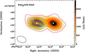
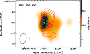
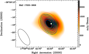
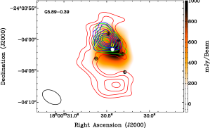
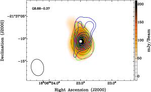
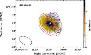
Fig. 1.— SMA line-free continuum maps at 1.3 mm (color scale) and velocity-integrated emission (moment 0, contours) of CH₃CN (12_K–11_K) for $K=3$ (red), $K=5$ (green) and $K=7$ (blue) lines. In all cases the contour levels have steps of 10% until 90% of the integrated emission shown in Table 6. For W3OH-H2O contour levels begin at 10% ($K=3$), 20% ($K=5$), and 50% ($K=7$). For I16547 contour levels begin at 40% ($K=3$), 50% ($K=5$), and 70% ($K=7$). For I17233 contour levels begin at 50% ($K=3$, $K=5$, and $K=7$). For G5.89 we used the $K$–lines 3, 5, and 6 with contour levels beginning at 30%, 40%, and 40%, respectively. For G5.89 the yellow box marks the position of the Feldt’s star (Feldt et al. 2003), and circles with crosses show condensations with excess 870 $\mu$m emission reported by Hunter et al. (2008). For G8.68 contour levels begin at 20% ($K=3$ and $K=5$) and 50% ($K=7$). For G10.47 contour levels begin at 20% ($K=3$ and $K=5$) and 40% ($K=7$). In all cases a white dot marks the peak position of 1.3 mm continuum emission (Table 3), and the synthesized beam (Table 3) is shown at the bottom-left.

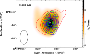
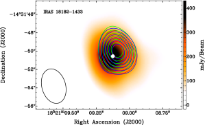
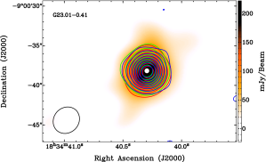
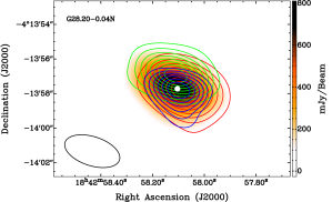
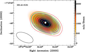
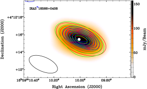
Fig. 2.— Continuation of Figure 1. For G10.62 contour levels begin at 20% ($K=3$, $K=5$, and $K=7$). For I18182 we used the $K$–lines 3, 5 and 6 with contour levels beginning at 50%. For G23.01 contour levels begin at 20% ($K=3$, $K=5$, and $K=7$). For G28.20 contour levels begin at 20% ($K=3$ and $K=5$), and 40% ($K=7$). For G31.41 contour levels begin at 40% ($K=3$, $K=5$, and $K=7$). For I18566 contour levels begin at 20% ($K=3$ and $K=5$), and 40% ($K=7$).

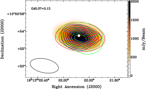
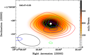
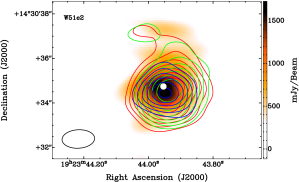
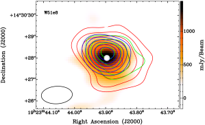
Fig. 3.— Continuation of Figure 1. For G45.07 contour levels begin at 20% ($K=3$ and $K=5$), and 30% ($K=7$). For G45.47 contour levels begin at 20% ($K=3$), 70% ($K=5$), and 50% ($K=7$). For W51e2 contour levels begin at 30% ($K=3$ and $K=5$), and 40% ($K=7$). For W51e8 contour levels begin at 30% ($K=3$), and 40% ($K=5$ and $K=7$).

Fig. 4.— Rotation diagrams for CH₃CN (12_K–11_K). The line is the linear fit of all data points in the plots. The numbers in the lower left panel, of W51e2, represent the $K-$ladder quantum numbers.

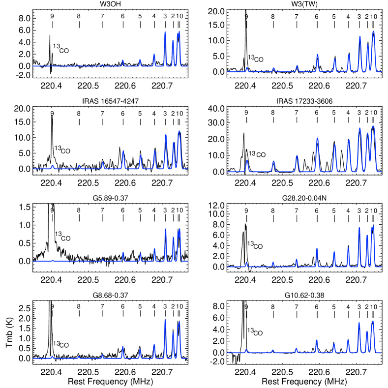
Fig. 5.— Observed CH₃CN (12_K–11_K) spectra (black) and synthetic model (blue) spectra obtained with XCLASS. The fit parameters are given in Table 4. The numbers in each panel represent the $K-$ladder quantum numbers. The line at $\sim$220.4 GHz is ¹³CO(2-1) and is overlapped with the $K=9$ line.

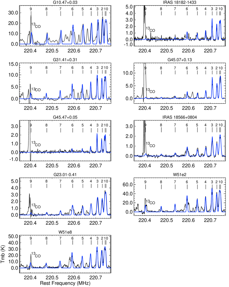
Fig. 6.— Continuation of Figure 5.

Fig. 7.— Plot of virial mass versus gas mass. $M_{\rm gas}$  is estimated from the 1.3 mm continuum emission using the high temperature of the CH₃CN analysis (Table 5). $M_{\rm vir}$ is estimated using $\Delta V$ from the observed linewidth (Table 4). The dotted line represents $M_{\rm vir}$/$M_{\rm gas}$ =1.

Fig. 8.— Fractional abundance of CH₃CN versus temperature of the compact hot and dense region estimated with XCLASS (squares). Uncertainties of the hot components were used to estimate uncertainties in gas masses and column densities from the continuum emission. For comparison, we plot our results from the rotational diagrams (crosses) and reported values for other HMCs (triangles). Reported data from the literature are taken from Galvan-Madrid et al. 2009, Chen et al. 2006, Wilner et al. 1994, Zhang et al. 1998, and Wang et al. 2010.

References

- Araya et al. (2005a) Araya, E., Hofner, P., Kurtz, S., Bronfman, L., & DeDeo, S. 2005a, ApJS, 157, 279
- Araya et al. (2005b) Araya, E., Hofner, P., Kurtz, S., Linz, H., Olmi, L., Sewilo, M., Watson, C., & Churchwell, E. 2005b, ApJ, 618, 339
- Araya et al. (2008) Araya, E., Hofner, P., Kurtz, S., Olmi, L., & Linz, H. 2008, ApJ, 675, 420
- Araya et al. (2007) Araya, E., Hofner, P., Sewiło, M., Linz, H., Kurtz, S., Olmi, L., Watson, C., & Churchwell, E. 2007, ApJ, 654, L95
- Argon et al. (2000) Argon, A. L., Reid, M. J., & Menten, K. M. 2000, ApJS, 129, 159
- Ballesteros-Paredes et al. (2011) Ballesteros-Paredes, J., Hartmann, L. W., Vázquez-Semadeni, E., Heitsch, F., & Zamora-Avilés, M. A. 2011, MNRAS, 411, 65, 1009.1583
- Beltrán et al. (2011) Beltrán, M. T., Cesaroni, R., Neri, R., & Codella, C. 2011, A&A, 525, A151, 1010.0843
- Beltrán et al. (2004) Beltrán, M. T., Girart, J. M., Estalella, R., & Ho, P. T. P. 2004, A&A, 426, 941, arXiv:astro-ph/0407102
- Beuther et al. (2002) Beuther, H., Walsh, A., Schilke, P., Sridharan, T. K., Menten, K. M., & Wyrowski, F. 2002, A&A, 390, 289, arXiv:astro-ph/0205348
- Beuther et al. (2009) Beuther, H., Walsh, A. J., & Longmore, S. N. 2009, ApJS, 184, 366, 0909.0691
- Beuther et al. (2006) Beuther, H., Zhang, Q., Sridharan, T. K., Lee, C., & Zapata, L. A. 2006, A&A, 454, 221, arXiv:astro-ph/0603814
- Caselli et al. (1993) Caselli, P., Hasegawa, T. I., & Herbst, E. 1993, ApJ, 408, 548
- Caswell & Haynes (1983) Caswell, J. L., & Haynes, R. F. 1983, JRASC, 77, 257
- Caswell & Vaile (1995) Caswell, J. L., & Vaile, R. A. 1995, MNRAS, 273, 328
- Cesaroni (2005) Cesaroni, R. 2005, in IAU Symposium, Vol. 227, Massive Star Birth: A Crossroads of Astrophysics, ed. R. Cesaroni, M. Felli, E. Churchwell, & M. Walmsley, 59–69
- Cesaroni et al. (2011) Cesaroni, R., Beltrán, M. T., Zhang, Q., Beuther, H., & Fallscheer, C. 2011, A&A, 533, A73, 1107.2849
- Cesaroni et al. (2010) Cesaroni, R., Hofner, P., Araya, E., & Kurtz, S. 2010, A&A, 509, A50
- Cesaroni et al. (1998) Cesaroni, R., Hofner, P., Walmsley, C. M., & Churchwell, E. 1998, A&A, 331, 709
- Cesaroni et al. (1994) Cesaroni, R., Olmi, L., Walmsley, C. M., Churchwell, E., & Hofner, P. 1994, ApJ, 435, L137
- Cesaroni et al. (1992) Cesaroni, R., Walmsley, C. M., & Churchwell, E. 1992, A&A, 256, 618
- Charnley et al. (1992) Charnley, S. B., Tielens, A. G. G. M., & Millar, T. J. 1992, ApJ, 399, L71
- Chen et al. (2006) Chen, H.-R., Welch, W. J., Wilner, D. J., & Sutton, E. C. 2006, ApJ, 639, 975, arXiv:astro-ph/0511294
- Churchwell et al. (1990) Churchwell, E., Walmsley, C. M., & Cesaroni, R. 1990, A&AS, 83, 119
- Churchwell et al. (1992) Churchwell, E., Walmsley, C. M., & Wood, D. O. S. 1992, A&A, 253, 541
- Comito et al. (2005) Comito, C., Schilke, P., Phillips, T. G., Lis, D. C., Motte, F., & Mehringer, D. 2005, ApJS, 156, 127
- De Buizer et al. (2005) De Buizer, J. M., Osorio, M., & Calvet, N. 2005, ApJ, 635, 452, arXiv:astro-ph/0508376
- Doty et al. (2002) Doty, S. D., van Dishoeck, E. F., van der Tak, F. F. S., & Boonman, A. M. S. 2002, A&A, 389, 446, arXiv:astro-ph/0205292
- Faúndez et al. (2004) Faúndez, S., Bronfman, L., Garay, G., Chini, R., Nyman, L.-Å., & May, J. 2004, A&A, 426, 97
- Feldt et al. (2003) Feldt, M. et al. 2003, ApJ, 599, L91
- Fish et al. (2005) Fish, V. L., Reid, M. J., Argon, A. L., & Zheng, X.-W. 2005, ApJS, 160, 220, arXiv:astro-ph/0505148
- Forster & Caswell (1989) Forster, J. R., & Caswell, J. L. 1989, A&A, 213, 339
- Franco-Hernández et al. (2009) Franco-Hernández, R., Moran, J. M., Rodríguez, L. F., & Garay, G. 2009, ApJ, 701, 974, 0906.3326
- Furuya et al. (2008) Furuya, R. S., Cesaroni, R., Takahashi, S., Codella, C., Momose, M., & Beltrán, M. T. 2008, ApJ, 673, 363, 0710.0029
- Furuya et al. (2005) Furuya, R. S., Cesaroni, R., Takahashi, S., Momose, M., Testi, L., Shinnaga, H., & Codella, C. 2005, ApJ, 624, 827, arXiv:astro-ph/0501644
- Galván-Madrid et al. (2009) Galván-Madrid, R., Keto, E., Zhang, Q., Kurtz, S., Rodríguez, L. F., & Ho, P. T. P. 2009, ApJ, 706, 1036, 0910.2270
- Garay et al. (2003) Garay, G., Brooks, K. J., Mardones, D., & Norris, R. P. 2003, ApJ, 587, 739
- Garay & Lizano (1999) Garay, G., & Lizano, S. 1999, PASP, 111, 1049, arXiv:astro-ph/9907293
- Gaume et al. (1993) Gaume, R. A., Johnston, K. J., & Wilson, T. L. 1993, ApJ, 417, 645
- Gaume & Mutel (1987) Gaume, R. A., & Mutel, R. L. 1987, ApJS, 65, 193
- Goddi et al. (2011) Goddi, C., Greenhill, L. J., Humphreys, E. M. L., Chandler, C. J., & Matthews, L. D. 2011, ApJ, 739, L13, 1106.4202
- Goldsmith & Langer (1999) Goldsmith, P. F., & Langer, W. D. 1999, ApJ, 517, 209
- Harju et al. (1998) Harju, J., Lehtinen, K., Booth, R. S., & Zinchenko, I. 1998, A&AS, 132, 211
- Hasegawa & Herbst (1993) Hasegawa, T. I., & Herbst, E. 1993, MNRAS, 263, 589
- Hatchell et al. (1998) Hatchell, J., Thompson, M. A., Millar, T. J., & MacDonald, G. H. 1998, A&AS, 133, 29
- Henning et al. (1995) Henning, T., Michel, B., & Stognienko, R. 1995, Planet. Space Sci., 43, 1333
- Herbst & van Dishoeck (2009) Herbst, E., & van Dishoeck, E. F. 2009, ARA&A, 47, 427
- Hildebrand (1983) Hildebrand, R. H. 1983, QJRAS, 24, 267
- Ho et al. (2004) Ho, P. T. P., Moran, J. M., & Lo, K. Y. 2004, ApJ, 616, L1, arXiv:astro-ph/0406352
- Hofner et al. (1999) Hofner, P., Peterson, S., & Cesaroni, R. 1999, ApJ, 514, 899
- Hunter et al. (2008) Hunter, T. R., Brogan, C. L., Indebetouw, R., & Cyganowski, C. J. 2008, ApJ, 680, 1271, 0803.0587
- Hunter et al. (2000) Hunter, T. R., Churchwell, E., Watson, C., Cox, P., Benford, D. J., & Roelfsema, P. R. 2000, AJ, 119, 2711
- Hunter et al. (1997) Hunter, T. R., Phillips, T. G., & Menten, K. M. 1997, ApJ, 478, 283
- Hunter et al. (1999) Hunter, T. R., Testi, L., Zhang, Q., & Sridharan, T. K. 1999, AJ, 118, 477
- Kalenskii et al. (1997) Kalenskii, S. V., Dzura, A. M., Booth, R. S., Winnberg, A., & Alakoz, A. V. 1997, A&A, 321, 311
- Kalenskii et al. (2000) Kalenskii, S. V., Promislov, V. G., Alakoz, A., Winnberg, A. V., & Johansson, L. E. B. 2000, A&A, 354, 1036
- Kaufman et al. (1998) Kaufman, M. J., Hollenbach, D. J., & Tielens, A. G. G. M. 1998, ApJ, 497, 276
- Keto et al. (1987) Keto, E. R., Ho, P. T. P., & Haschick, A. D. 1987, ApJ, 318, 712
- Keto et al. (1988) ——. 1988, ApJ, 324, 920
- Klaassen et al. (2009) Klaassen, P. D., Wilson, C. D., Keto, E. R., & Zhang, Q. 2009, ApJ, 703, 1308, 0907.4377
- Kurtz et al. (2000) Kurtz, S., Cesaroni, R., Churchwell, E., Hofner, P., & Walmsley, C. M. 2000, Protostars and Planets IV, 299
- Leurini et al. (2011) Leurini, S., Codella, C., Zapata, L., Beltrán, M. T., Schilke, P., & Cesaroni, R. 2011, A&A, 530, A12, 1104.0857
- Leurini et al. (2009) Leurini, S. et al. 2009, A&A, 507, 1443, 0909.0525
- Linke et al. (1979) Linke, R. A., Frerking, M. A., & Thaddeus, P. 1979, ApJ, 234, L139
- Liu et al. (2011) Liu, H. B., Zhang, Q., & Ho, P. T. P. 2011, ApJ, 729, 100, 1101.3459
- Longmore et al. (2011) Longmore, S. N., Pillai, T., Keto, E., Zhang, Q., & Qiu, K. 2011, ApJ, 726, 97, 1011.1442
- MacDonald & Habing (1995) MacDonald, G. H., & Habing, R. J. 1995, in Lecture Notes in Physics, Berlin Springer Verlag, Vol. 459, The Physics and Chemistry of Interstellar Molecular Clouds, ed. G. Winnewisser & G. C. Pelz, 291–293
- MacLaren et al. (1988) MacLaren, I., Richardson, K. M., & Wolfendale, A. W. 1988, ApJ, 333, 821
- Mookerjea et al. (2007) Mookerjea, B., Casper, E., Mundy, L. G., & Looney, L. W. 2007, ApJ, 659, 447, arXiv:astro-ph/0701827
- Müller et al. (2005) Müller, H. S. P., Schlöder, F., Stutzki, J., & Winnewisser, G. 2005, Journal of Molecular Structure, 742, 215
- Müller et al. (2001) Müller, H. S. P., Thorwirth, S., Roth, D. A., & Winnewisser, G. 2001, A&A, 370, L49
- Nummelin et al. (2000) Nummelin, A., Bergman, P., Hjalmarson, Å., Friberg, P., Irvine, W. M., Millar, T. J., Ohishi, M., & Saito, S. 2000, ApJS, 128, 213
- Ohishi & Kaifu (1998) Ohishi, M., & Kaifu, N. 1998, Faraday Discussions, 109, 205
- Olmi et al. (1993) Olmi, L., Cesaroni, R., & Walmsley, C. M. 1993, A&A, 276, 489
- Olmi et al. (1996) ——. 1996, A&A, 307, 599
- Osorio et al. (2009) Osorio, M., Anglada, G., Lizano, S., & D’Alessio, P. 2009, ApJ, 694, 29, 0811.4096
- Osorio et al. (1999) Osorio, M., Lizano, S., & D’Alessio, P. 1999, ApJ, 525, 808
- Ossenkopf & Henning (1994) Ossenkopf, V., & Henning, T. 1994, A&A, 291, 943
- Pandian et al. (2008) Pandian, J. D., Momjian, E., & Goldsmith, P. F. 2008, A&A, 486, 191, 0805.2697
- Pankonin et al. (2001) Pankonin, V., Churchwell, E., Watson, C., & Bieging, J. H. 2001, ApJ, 558, 194
- Pickett et al. (1998) Pickett, H. M., Poynter, R. L., Cohen, E. A., Delitsky, M. L., Pearson, J. C., & Müller, H. S. P. 1998, J. Quant. Spec. Radiat. Transf., 60, 883
- Polushkin & Val’Tts (2011) Polushkin, S. V., & Val’Tts, I. E. 2011, Astronomy Reports, 55, 445
- Purcell et al. (2006) Purcell, C. R. et al. 2006, MNRAS, 367, 553, arXiv:astro-ph/0512589
- Purcell et al. (2013) ——. 2013, ApJS, 205, 1, 1211.7116
- Qin et al. (2008) Qin, S.-L., Huang, M., Wu, Y., Xue, R., & Chen, S. 2008, ApJ, 686, L21, 0808.3443
- Qin et al. (2010) Qin, S.-L., Wu, Y., Huang, M., Zhao, G., Li, D., Wang, J.-J., & Chen, S. 2010, ApJ, 711, 399
- Reid et al. (2014) Reid, M. J. et al. 2014, ArXiv e-prints, 1401.5377
- Reid et al. (2009) ——. 2009, ApJ, 700, 137, 0902.3913
- Remijan et al. (2004a) Remijan, A., Shiao, Y.-S., Friedel, D. N., Meier, D. S., & Snyder, L. E. 2004a, ApJ, 617, 384
- Remijan et al. (2004b) Remijan, A., Sutton, E. C., Snyder, L. E., Friedel, D. N., Liu, S.-Y., & Pei, C.-C. 2004b, ApJ, 606, 917
- Rodgers & Charnley (2001) Rodgers, S. D., & Charnley, S. B. 2001, ApJ, 546, 324
- Rodríguez et al. (2008) Rodríguez, L. F., Moran, J. M., Franco-Hernández, R., Garay, G., Brooks, K. J., & Mardones, D. 2008, AJ, 135, 2370, 0804.0858
- Rolffs et al. (2011) Rolffs, R., Schilke, P., Zhang, Q., & Zapata, L. 2011, A&A, 536, A33
- Sanna et al. (2010) Sanna, A., Moscadelli, L., Cesaroni, R., Tarchi, A., Furuya, R. S., & Goddi, C. 2010, A&A, 517, A78, 1004.5578
- Schilke et al. (1999) Schilke, P., Phillips, T. G., & Mehringer, D. M. 1999, in The Physics and Chemistry of the Interstellar Medium, ed. V. Ossenkopf, J. Stutzki, & G. Winnewisser, 330
- Sollins & Ho (2005) Sollins, P. K., & Ho, P. T. P. 2005, ApJ, 630, 987, arXiv:astro-ph/0506057
- Sollins et al. (2004) Sollins, P. K. et al. 2004, ApJ, 616, L35, arXiv:astro-ph/0403524
- Sollins et al. (2005a) Sollins, P. K., Zhang, Q., Keto, E., & Ho, P. T. P. 2005a, ApJ, 631, 399, arXiv:astro-ph/0506059
- Sollins et al. (2005b) ——. 2005b, ApJ, 624, L49, arXiv:astro-ph/0410604
- Solomon et al. (1971) Solomon, P. M., Jefferts, K. B., Penzias, A. A., & Wilson, R. W. 1971, ApJ, 168, L107
- Su et al. (2009) Su, Y.-N., Liu, S.-Y., Wang, K.-S., Chen, Y.-H., & Chen, H.-R. 2009, ApJ, 704, L5, 0908.3924
- Turner (1991) Turner, B. E. 1991, ApJS, 76, 617
- Viti et al. (2004) Viti, S., Collings, M. P., Dever, J. W., McCoustra, M. R. S., & Williams, D. A. 2004, MNRAS, 354, 1141, arXiv:astro-ph/0406054
- Walsh et al. (1998) Walsh, A. J., Burton, M. G., Hyland, A. R., & Robinson, G. 1998, MNRAS, 301, 640
- Wang et al. (2010) Wang, K.-S., Kuan, Y.-J., Liu, S.-Y., & Charnley, S. B. 2010, ApJ, 713, 1192
- Wilner et al. (2001) Wilner, D. J., De Pree, C. G., Welch, W. J., & Goss, W. M. 2001, ApJ, 550, L81
- Wilner et al. (1995) Wilner, D. J., Welch, W. J., & Forster, J. R. 1995, ApJ, 449, L73+
- Wilner et al. (1994) Wilner, D. J., Wright, M. C. H., & Plambeck, R. L. 1994, ApJ, 422, 642
- Wink et al. (1994) Wink, J. E., Duvert, G., Guilloteau, S., Gusten, R., Walmsley, C. M., & Wilson, T. L. 1994, A&A, 281, 505
- Wyrowski et al. (1999a) Wyrowski, F., Schilke, P., & Walmsley, C. M. 1999a, A&A, 341, 882
- Wyrowski et al. (1999b) Wyrowski, F., Schilke, P., Walmsley, C. M., & Menten, K. M. 1999b, ApJ, 514, L43, arXiv:astro-ph/9901261
- Zapata et al. (2009) Zapata, L. A., Ho, P. T. P., Schilke, P., Rodríguez, L. F., Menten, K., Palau, A., & Garrod, R. T. 2009, ApJ, 698, 1422, 0904.0325
- Zapata et al. (2008) Zapata, L. A., Leurini, S., Menten, K. M., Schilke, P., Rolffs, R., & Hieret, C. 2008, AJ, 136, 1455, 0807.1591
- Zapata et al. (2006) Zapata, L. A., Rodríguez, L. F., Ho, P. T. P., Beuther, H., & Zhang, Q. 2006, AJ, 131, 939, arXiv:astro-ph/0510761
- Zapata et al. (2011) Zapata, L. A., Schmid-Burgk, J., & Menten, K. M. 2011, A&A, 529, A24, 1009.1426
- Zhang & Ho (1995) Zhang, Q., & Ho, P. T. P. 1995, ApJ, 450, L63
- Zhang & Ho (1997) ——. 1997, ApJ, 488, 241
- Zhang et al. (1998) Zhang, Q., Ho, P. T. P., & Ohashi, N. 1998, ApJ, 494, 636
- Zhang et al. (2007) Zhang, Q., Sridharan, T. K., Hunter, T. R., Chen, Y., Beuther, H., & Wyrowski, F. 2007, A&A, 470, 269, 0704.2767