Information under Lorentz transformation

Abstract

A general form of a two-qubit system is obtained under the effect of Lorentz transformation. We investigate extensively some important classes in the context of quantum information. It is shown Lorentz transformation causes a decay of entanglement and consequently information loses. On the other hand, it generates entangled states between systems prepared initially in a separable states. The partial entangled states are more robust under Lorentz transformation than maximally entangled states. Therefore the rate of information lose is larger for maximum entangled states compared with that for partially entangled states.

I Introduction

It is now well known that the increase of the classical computers speed has physical limitations chen . These limitations are fundamentally encrypted in the quantum mechanical effects. Since few decades several groups are developing a new concept of information processing, quantum information processing, in order to overcome the classical information processing limitations chen ; Nielsen . One of the most powerful tools for the quantum computing is the entanglement, a pure quantum effect allowing to speed up the quantum algorithms and to exchange the information in non classical way. In the last two decades a large number of works has been done to study the entanglement in physical systems Xiao ; Eskandari ; Soares ; el1 ; aty1 ; kim02 . However almost all these contributions were limited to the non-relativistic effects. Since the development of the special relativity Einstein the way of looking to the dynamical systems with high speed is drastically changed. Dirac Dirac ; Dirac2 introduced the relativistic effect in quantum mechanics just few years of the establishing its concepts and foundations.

Recently there are some achievements on relativistic quantum information. For example, Saldanha and Vedral Saldanaha2012 show that a massive 2- qubit particles prepared in a maximally entangled state is not capable of maximally violating the Clouser-Horne Shimony-Holt inequality. A scheme for storing quantum information in the field modes of moving cavities in non-inertial frames was reported Downes . Choi investigated the relativistic effects on the spin of entanglement of two massive Dirac particles Choi2011 . The effect of the special relativity on the entanglement between spins and momenta of two-qubit system is investigated by Cafaro et. al. Cafaro2012 . Some properties of a system of two-spin -1 particles under Lornetz transformation have investigated by Ruiz and E. N.-Achar Esteban2012

In this work we study, in the relativistic context, the dynamical behavior of the entanglement for some particular and important classes of initial states of two-qubit system, namely Werner, $x-$ and generic pure states. We analyze the dynamical evolution of the entropy and the information loses for this system. We show that non-intuitive results are emerging from the relativistic transformation.

The paper is organized as follows. In Sec. 2, a short review of the effect of Lorentz transformation on a two qubits state is presented. In Sec. 3, we describe the couplings between the two qubits, and then we obtain the Bloch vectors under the effect of the lorentz transformation. In Sec. 4, we discuss how to characterize the quantum entanglement by using the concurrence, in contrast to the Werner state and Bell states. In Sec. 5, the basic principle of information loss is discussed. In particular, we discuss the effect of Lornetz transformation on the local and non local information via calculating the entropy of both subsystems and the total state. Finally, we summary the main results of the paper in Sec. 6.

II Model Description and Lorentz Transformation

In this section we review the effect of Lorentz transformation on a two qubits state given in the rest frame as:

$$\bigl{|}\Psi\bigr{\rangle}=\bigl{|}\psi_{p_{a}}\bigr{\rangle}\bigl{|}\psi_{p_{b}}\bigr{\rangle}\bigl{|}\psi_{s}\bigr{\rangle},$$ (1)

where$\bigl{|}\psi_{p_{a}}\bigr{\rangle}$ and $\bigl{|}\psi_{p_{b}}\bigr{\rangle}$ are the momentum states for the first and the second qubit respectively, while $\bigl{|}\psi_{s}\bigr{\rangle}$ represents the spin state vector for both particles Hui . A Lorentz transformation $\Lambda$ changes $\bigl{|}\psi_{p_{i}}\bigr{\rangle}$ to $\bigl{|}\Lambda\psi_{p_{i}}\bigr{\rangle}$, where $i=a,b$. This transformation represents a unitary operator on the space of momenta spaceJordan . Therefore the Lorentz transformation change the state(1) as:

$$\bigl{|}\Psi^{\prime}\bigr{\rangle}=\bigl{|}\Lambda\psi_{p_{a}}\bigr{\rangle}\bigl{|}\Lambda\psi_{p_{b}}\bigr{\rangle}\mathcal{U}_{a}(\psi_{pa})\mathcal{U}_{b}(\psi_{pb})\bigl{|}\psi_{s}\bigr{\rangle},$$ (2)

where,$\mathcal{U}_{a}$ and $\mathcal{U}_{b}$ are operators on the spin states for both particles. In the computational basis $\bigl{|}00\bigr{\rangle},\bigl{|}01\bigr{\rangle},\bigl{|}10\bigr{\rangle}$ and $\bigl{|}11\bigr{\rangle}$, the operator $\mathcal{U}=\mathcal{U}_{a}\otimes\mathcal{U}_{b}$ can be written as

$$\mathcal{U}=\bigl{|}00\bigr{\rangle}\bigl{\langle}00\bigr{|}+\bigl{|}11\bigr{\rangle}\bigl{\langle}11\bigr{|}+e^{-i\phi}\bigl{|}01\bigr{\rangle}\bigl{\langle}10\bigr{|}+e^{i\phi}\bigl{|}10\bigr{\rangle}\bigl{\langle}10\bigr{|}.$$ (3)

Assume that a source supplies two users Alice and Bob with a two qubits of massive Dirac particles. The spin part of this system is defined by $15$ parameters: $6$ of them represent Bloch vectors for the first and the second qubits respectively. The other nine parameters represent the component of the correlation tensor metwally .

$$\rho_{ab}=\frac{1}{4}\left(1+\sum_{i=1}^{3}{s_{i}\sigma_{i}}+\sum_{j=1}^{3}{t_{j}\tau_{j}}+\sum_{ij=1}^{3}{c_{ij}\sigma_{i}\tau_{j}}\right),$$ (4)

where $\sigma_{i},\tau_{j}$, $i,j=1,2,3$ are the Pauli matrices for the first and second’s qubit respectively, $s_{i},t_{j}$ with $s_{i}=tr\{\rho_{ab}\sigma_{i}\}$ and $t_{j}=tr\{\rho_{ab}\tau_{j}\}$ are Bloch vectors for both qubits respectively. The tensor correlation is defined by a $3\times 3$ matrix with elements are defined by $c_{ij}=tr\{\rho_{ab}\sigma_{i}\tau_{j}\}$. For example, $c_{11}=tr\{\rho_{ab}\sigma_{1}\tau_{1}\},c_{x12}=tr\{\rho_{ab}\sigma_{1}\tau_{2}\},c_{13}=tr\{\rho_{ab}\sigma_{1}\tau_{3}\}$ and so on. From the general form (4), one can obtains different classes metwally1 .

The dynamics of the state (4) under the effect of the lorentz transformation is characterized by its new Bloch vectors,

$$\tilde{s}_{1} = s_{1}\cos\phi-s_{2}\sin\phi,\quad\tilde{s}_{2}=s_{2}\cos\phi-s_{1}\sin\phi,\quad\tilde{s}_{3}=\frac{s_{3}}{2}(1+\cos 2\phi)+\frac{t_{3}}{2}(1-\cos 2\phi),$$

$$\tilde{t}_{1} = t_{1}\cos\phi-t_{2}\sin\phi,\quad\tilde{t}_{2}=t_{1}\sin\phi+t_{2}\cos\phi,\quad\tilde{t}_{3}=\frac{s_{3}}{2}(1-\cos 2\phi)+\frac{t_{3}}{2}(1+\cos 2\phi),$$

and the $9$ elements of the cross dyadic which are defined as,

$$\tilde{c}_{xx} = \frac{1}{2}(1+\cos 2\phi)c_{xx}+\frac{1}{2}(1-\cos 2\phi)c_{yy}+\frac{1}{2}(c_{xy}-c_{yx})\sin 2\phi,$$

$$\tilde{c}_{xy} = \frac{1}{2}(1+\cos 2\phi)c_{xy}+\frac{1}{2}(1-\cos 2\phi)c_{yx}-\frac{1}{2}(c_{xx}+c_{yy})\sin 2\phi,$$

$$\tilde{c}_{xz} = \cos\phi~{}c_{xz}-\sin\phi~{}c_{yz},$$

$$\tilde{c}_{yx} = \frac{1}{2}(1+\cos 2\phi)c_{yx}+\frac{1}{2}(1-\cos 2\phi)c_{xy}+\frac{1}{2}(c_{xx}+c_{yy})\sin 2\phi,$$

$$\tilde{c}_{yy} = \frac{1}{2}(1+\cos 2\phi)c_{yy}-\frac{1}{2}(1-\cos 2\phi)c_{xx}-\frac{1}{2}(c_{xy}+c_{yx})\sin 2\phi,$$

$$\tilde{c}_{yz} = \cos\phi~{}c_{yz}+\sin\phi~{}c_{xz},$$

$$\tilde{c}_{zx} = \cos\phi~{}c_{zx}+\sin\phi~{}c_{zy},\quad\quad\tilde{c}_{zy}=\cos\phi~{}c_{zy}+\sin\phi~{}c_{zx},~{}\quad\tilde{c}_{zz}=c_{zz}.$$ (6)

In the following section we shall consider some important example in context of quantum information as Werner state, $x-$ state and a generic pure state, were we investigate the dynamics of these states under the effect of Lorentz transformation. Also, we quantify the degree of entanglement of the new states.

III Entanglement

In this section, we quantify the degree of entanglement under the effect of Lorentz transformation. We use Wootters’concurrence Woottors , for this propose, which is defined as,

$$\mathcal{E}=\max\Bigl{\{}0,\lambda_{1}-\lambda_{2}-\lambda_{3}-\lambda_{4}\Bigr{\}},$$ (7)

where $\lambda_{1}\geq\lambda_{2}\geq\lambda_{3}\geq\lambda_{4}$ and $\lambda_{i}$ are the eigenvalues of the density operator $\rho=\sigma_{2}\tau_{2}\rho^{*}\sigma_{2}\tau_{2}$, $\rho^{*}$ is the complex conjugate of $\rho$.

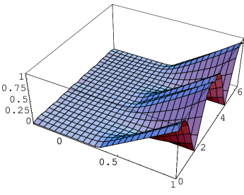
Figure 1: The dynamics of entanglement under Lorentz transformation for a system is initially prepared in different classes of Werner states

1. X-state: This class of states Eberly represents one of most important classes in the context of quantum information Chen ; Ali ; Rau ; Alaa . On the other hand, from this class, one can generate Werner state and Bell states. The density operator of this class is given by,

   $$\rho_{x}=\frac{1}{4}(1+c_{xx}\sigma_{x}\tau_{x}+c_{yy}\sigma_{y}\tau_{y}+c_{zz}\sigma_{z}\tau_{z})$$ (8)

   Under Lorentz transformation, this state (8) is transformed into

   $$\tilde{\rho}_{x} = \frac{1}{4}\Bigl{\{}1+\frac{1}{2}\{(1+\cos 2\phi)c_{xx}+(1-\cos 2\phi)c_{yy}\}\sigma_{x}\tau_{x}-\frac{1}{2}(c_{xx}+c_{yy})sin2\phi(\sigma_{x}\tau_{y}-\sigma_{y}\tau_{x})$$ (9)

   $$\hskip 28.45274pt-\frac{1}{2}\{(1-\cos 2\phi)c_{xx}-(1+\cos 2\phi)c_{yy}\}\sigma_{y}\tau_{y}+c_{zz}\sigma_{z}\tau_{z}\Bigl{\}}$$

   Fig.(1) shows the behavior of entanglement of Werner state Wer , where this state is initially defined by its zero Bloch vectors, i.e., $\mathord{\buildrel\lower 3.0pt\hbox{$\scriptscriptstyle\rightarrow$}\over{s}}=\mathord{\buildrel\lower 3.0pt\hbox{$\scriptscriptstyle\rightarrow$}\over{t}}=0$ and $c_{xx}=c_{yy}=c_{zz}=-x$. It has been shown that has been shown that this state is separable for $x\in[-\frac{1}{3},\frac{1}{3}]$ and nonseparable for $\frac{1}{3}<x\leq 1$ (see for example metally).

   For entangled state classes i.e., $x\in[\frac{1}{3},1]$, the entanglement decreases to reach its minimum value as $\varphi$ increases. Then the entanglement re-birthed again to reach its maximum bound. This maximum bound depends on the value of the parameter $x$, where Werener state represents a singlet state (Bell state) at $x=1$, which is a maximum entangled state.

   On the other hand, for separable classes namely for any $x\in[-\frac{1}{3},\frac{1}{3}]$, the separable states turns into entangled states as shown in Fig. 1b. However the degree of entanglement is smaller than those depicted for initially entangled classes.

   

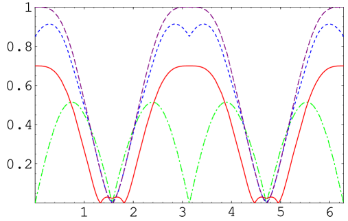
   Figure 2: The dynamics of entanglement under Lorentz transformation for a system is initially prepared in maximum entangled states (dash-dot curve), Werner state with $x=-0.6$ (solid curves) and $X$-states with (dot ) curves $c_{xx}=-0.9,c_{yy}=-0.8$ and $c_{zz}=-0.7$.

   Fig.(2) shows the effect of Lorentz transformation on the degree of entanglement for maximum entangled state, where $c_{xx}=c_{yy}=c_{zz}=-1$, x-state which defined by $c_{xx}=-0.9\neq c_{yy}=-0.8\neq c_{zz}=-0.7$ and Werner state with $c_{xx}=c_{yy}=c_{zz}=0.7$. As a general behavior, the entanglement $\mathcal{E}$ decreases as $\phi$ increase. The decreasing rate depends on the degree of entanglement for the initial state. However for maximum entangled sates, MES the entanglement decreases very fast to completely vanish and then re-birth again to reach its maximum value $(\mathcal{E}=1$). For less entangled states, a similar behavior is depicted as MES, but the entanglement is complectly death for longer interval of $\phi$. Also, this figure shows the effect of Lorentz transformation on systems prepared initially in a separable states, where we set $x=-0.6$. It is clear that the initial entanglement is zero. However as $\varphi$ increases an entangled state is generated and its maximum value is $\mathcal{E}\simeq 0.44$.

2. Generic pure state

   This state is described by the density operatormetwally ,

   $$\rho_{p}=\frac{1}{4}(1+p(\sigma_{x}-\tau_{x})-\sigma_{x}\tau_{x}-q(\sigma_{y}\tau_{y}+\sigma_{z}\tau_{z})),$$ (10)

   where, $q=\sqrt{1-p^{2}}$ . Under the Lorentez transformation this state is transformed into

   $$\tilde{\rho}_{p} = \frac{1}{4}\Bigl{\{}1+p\cos\phi(\sigma_{x}-\tau_{x})-\frac{1}{2}\{(1+q)+(1-q)\cos 2\phi\}\sigma_{x}\tau_{x}+\frac{1}{2}(1+q)\sin 2\phi\sigma_{x}\tau_{y}$$ (11)

   $$- \frac{1}{2}(1-q)\sin 2\phi\sigma_{y}\tau_{x}+\frac{1}{2}\{(1-q)-(1+q)\cos 2\phi\}\sigma_{y}\tau_{y}-q\sigma_{z}\tau_{z}\Bigr{\}}.$$

   

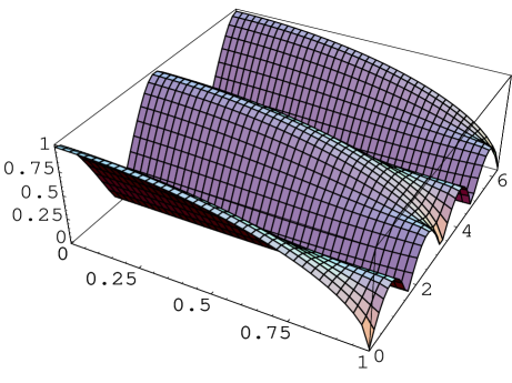
   Figure 3: The same as Fig.(1) but for a system is prepared initially in a pure state.

   

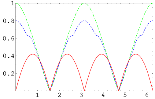
   Figure 4: The dynamics of Entanglement $\mathcal{E}$ for a system prepared initially in a pure state. The dash-dot curve for $p=0$ (MES), dot curve for PES with $p=0.6$ and the solid curve for separable state i.e., $p=1$.

IV Information loss

In this section, we investigate the effect of Lornetz transformation on the local and non local information via calculating the entropy of both subsystems and the total state. The entropy of a a density operator $\rho$ is defined by Von Numman entropy $\mathcal{P}_{n}=-\varrho ln\varrho$. This value indicate how much of information that the state $\varrho$ is lost.

In Fig. 4, we investigate the dynamics of entropy of different classes of Werner type under the effect of Lorentz transformation. It is clear that starting from entangled classes i.e., $\frac{1}{3}<x\leq 1$, the initial entropy is not maximum. This means that these state contains some quantum information. As $x$ increases the entropy $\mathcal{P}_{n}$ decreases to reach its minimum values at $x=1$ i.e., the initial state is maximum entangled state. On the other hand, as one increases $\varphi$, the entropy increases faster for larger values of $x$, namely classes with larger degree of entanglement. However for less entangled states the entropy is slightly increases. This show that the less entangled classes are more robust under Lorentz transformation. These results are shown in Fig. 4a. Starting from a separable classes, the initial entropy $\mathcal{P}_{n}$ is larger than that for entangled states. However, the entropy reaches its maximum value for less entangled states as shown in Fig. $4b$. Also, as one increases $\varphi$, the entropy $\mathcal{P}_{n}$ oscillates between its maximum and minimum values.

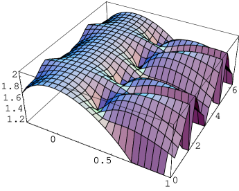
Figure 5: The behavior of entropy $\mathcal{P}_{n}$ under Lorentz transformation for different classes of Werner state

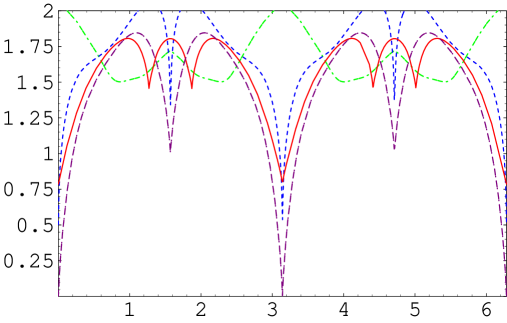
Figure 6: The behavior of Entropy $\mathcal{P}_{n}$ under Lorentz transformation for a system is initially prepared in maximum entangled states (dash- curve), Werner state with $x=-0.6$ (dash-dot) and $x=0.7$ (dot curve) and $X$-states with (solid ) curves $c_{xx}=-0.9,c_{yy}=-0.8$ and $c_{zz}=-0.7$ (solid-curve).

Fig. 5 shows the behavior of the entropy of different classes of the $x-$ state (8). It is clear that, starting from a maximum entangled class, i.e., we set $c_{xx}=c_{yy}=c_{zz}=-1$, the entropy $\mathcal{P}_{n}=0$ at $\varphi=0$. This means that the amount of information on this state is maximum. However as one increases $\varphi$, the entropy increases on the expanse of the non-local information to reach its maximum values $(\mathcal{P}_{n}=2)$. This maximum value is reached at $\varphi\simeq\frac{\pi}{3}$ i.e., at the same value of the minimum amount of entanglement (see Fig. 2). Also, this figure depicts the behavior of entropy for a class of Werner state, where we set $c_{xx}=c_{yy}=c_{zz}=x=0.7$ i.e., the initial state represents a partial entangled state with small degree of entanglement, the initial value of entropy is larger than that depicted for maximum entangled state. As one increases the Lornetz transformation’s parameter $\varphi$, the entropy decreases to reach its minimum value and increases again. However for this class the minimum value always larger than the initial values. The behavior of entropy starting from a separable class of Werner type, where we set $x=-0.6$, the initial entropy is maximum, i.e., $\mathcal{P}_{n}=2$. However this entropy oscillates between minimum and maximum values as $\varphi$ increases. This show that there is an entangled state is generated for different values of $\varphi$. Finally this figure depict the behavior of entropy under the effect of Lorentz transformation for a class of $x-$ states i.e., $c_{xx}\neq c_{yy}\neq c_{zz}$. It is clear that a similar behavior is shown as the pervious classes, but the entropy doesn’t reach its maximum value. So, this class is more robust than the previous class under the effect of Lorentz transformation.

V Conclusion

In this contribution obtain an analytical form for the spin part of the a general two-qubit systems. Some classes as Werner, $x-$ and a generic pure states are investigated extensively. The behavior of entanglement as well as the entropy which measures the information loses are investigated. It is shown that, the degree of entanglement decreases faster to completely vanish for system s prepared initially in maximum entangled states. Starting from less entangled states, the entanglement decreases gradually to reach its minimum value. On the other hand, the entanglement rebirth faster for the systems prepared initially in maximum entangled states. As one increases the lorentz parameter, the re-birth entanglement doesn’t exceeds its initial values. Our results show that one can generate entangled states starting from systems prepared initially in a separable states. In this case the generated entangled states depends on the structures of the initial systems. It is clear that, starting from a separable state generated from a pure state has a larger degree of entanglement compared with that obtained from Werner classes. The information loss is quantified by investigating the behavior of entropy for different classes of initial states. It is clear that the entropy of systems prepared initially in a partially entangled states increases gradually, but it increases fast for systems prepared initially in maximum entangled states. Therefore partially entangled states are more robust than maximum entangled states and consequently the rate of information loss is larger for maximum entangled states compared with that for partially entangled states.

References

- (1) Goong Chen, David A. Church, Berthold-Georg Englert, Carsten Henkel, Bernd Rohwedder, Marlan O. Scully, M. Suhail Zubairy, Quantum Computing Devices: Principles, Designs, and Analysis, Chapman & Hall/CRC Applied Mathematics & Nonlinear Science, Taylor and Francis Group, New York, 2007.
- (2) M. A. Nielsen, and I. L. Chuang, Quantum computation and quantum information. Cambridge University Press, 2000.
- (3) M. S. Kim, G. S. Agarwal, Phys. Rev. A 59, 3044 (1999).
- (4) XQ. Xiao, J. Zhu, GQ. He, GH. Zeng, Quant. Inf. Process. 12, 449(2013).
- (5) M. R. Eskandari, L. Rezaee, Int. J. Mod. Phys. B 26, 1250184(2012).
- (6) D. O. Soares-Pinto, R. Auccaise, J. Maziero, A. Gavini-Viana, R. M. Serra, L. C. Celeri, Phil. Trans. Roy. Soc. A 370 (2012) 4821.
- (7) H. Eleuch, Int. J. Mod. Phys. B 24, 5653(2010).
- (8) M. Abdel-Aty, J. Larson, H. Eleuch, A. S. F. Obada, Physica E 43, 1625 (2011).
- (9) M. S. Kim , W. Son, V. Buzek, P. L. Knight, Phys. Rev. A 65, 032323 (2002).
- (10) A. Einstein, Annalen der Physik 17, 891 (1905).
- (11) P. A. M. Dirac, Proc. R. Soc. Lond. A 117, 610 (1928).
- (12) P. A. M. Dirac, Proc. R. Soc. Lond. A. 118, 779 (1928).
- (13) P. Saldanaha and V. Vedral, Phys. Rev. A 85 062101 (2012).
- (14) T. G. Downes, I. Fuentes and T. C. G. Sudarshan, Phys. Rev. Lett. 106 210502 (2011).
- (15) T. Choi, Phys. Rev. a 84 012334 (2011).
- (16) C. Cafaro, S. Capozziello and S. Mancini, Int. J. Theor Phys. 51 2313 (2012).
- (17) E. C.-Ruiz and E. N.-Achar, Phys. Rev. A86 052331 (2012).
- (18) Hui-Li and Jiangfeng Du, Phys. Rev. A 68, 022108 (2003).
- (19) T. F. Jordan, A. Shaji and E. C. G. Sudarshan, Phys. Rev. A 75, 022101 (2007).
- (20) B.-G. Englert and N. Metwally, J. Mod. Opt. 47, 221 (2000);B.-G. Englert and N. Metwally, Appl. Phys B 72, 35 (2001).
- (21) N. Metwally, ”Information Loss in Local Dissipation Environments,” Int. J. Theor. Phys. 49, 1571, (2010), N. Metwally, Quantum Physics, arXiv:1201.5941 (2012).
- (22) S. Hill and W. K. Wootters, Phys. Rev. Lett. 78 5022 (1997); W. K. Wootters W K, Phys. Rev. Lett. 80 2245 (1998).
- (23) R. F. Werner, Phys. Rev. A 40, 4277 (1989).
- (24) T.Yu and J.H.Eberly, Quantum Inform. Comput. 7, 459 (2007).
- (25) Qing Chen, C. Zhang, S. Yu, X.X. Yi and C.H. Oh, Phys. Rev. A 84, 042313 (2011).
- (26) M. Ali, A. R. P. Rau and G. A, Phys. Rev. A 81, 042105 (2010).
- (27) M. Ali, G. Alber and A. R. P. Rau, J. Phys. B 42, 025501 (2009).
- (28) N. Metwally and A. Al-Sagheer, arXiv:1302.7295(2013).