New Lagrangian diagnostics for characterizing fluid flow mixing

Abstract

A new kind of Lagrangian diagnostic family is proposed and a specific form of it is suggested for characterizing mixing: the maximal extent of a trajectory (MET). It enables the detection of coherent structures and their dynamics in two- (and potentially three-) dimensional unsteady flows in both bounded and open domains. Its computation is much easier than all other Lagrangian diagnostics known to us and provides new insights regarding the mixing properties on both short and long time scales and on both spatial plots and distribution diagrams. We demonstrate its applicability to two dimensional flows using two toy models and a data set of surface currents from the Mediterranean Sea.

I Introduction

Visualizing and quantifying mixing in unsteady fluid flows is a magical and tricky business, with important practical implications including larval dispersion and population connectivity Gawarkiewicz et al. (2007); BozorgMagham et al. (2013), oil spills Mezic et al. (2010); Olascoaga and Haller (2012), search and rescue Peacock and Haller (2013); Melsom et al. (2012), functioning of the marine ecological system D’ovidio et al. (2009) and more Mariano et al. (2002). By now there are many tools to visualize and analyze mixing properties of flows and maps Aref (2002); Ottino (1989); Mancho et al. (2006); Beron-vera and Olascoaga (2009); Koshel and Prants (2006); Peacock and Dabiri (2010); Bollt and Santitissadeekorn (2013); Prants (2013); Budišić et al. (2012). While this field provides an endless source of scientifically produced art, beyond its aesthetic nature lurks the scientific challenge of characterizing these complex phenomena and providing predictions and insights relevant for real life problems.

One aspect of the complexity arises from the flow field structure. Unsteady flow fields typically have a mixture of Coherent Structures (CSs), jets and mixing layers that move in an unsteady fashion. Moreover, these structures may exist for some finite time. Roughly, by coherent structure we mean a body of fluid which moves together for a certain period of time, namely, we take the Lagrangian point of view which is frame independent (see discussion and references in Bollt and Santitissadeekorn (2013); Poje and Haller (1999); Haller and Beron-Vera (2013)). Passive particles placed inside such a coherent structure remain in it as long as it lives, moving roughly quasi-periodically around the coherent structure center. Here we mainly focus on such CSs. Jets may be similarly characterized as regular particles that flow between neighboring sections. These structures are typically separated by mixing layers, the regions in which there is “chaotic mixing” - a sensitive dependence of the Lagrangian trajectories on initial conditions (i.c.). Particles belonging to the mixing layer may stick to a nearby coherent structure or a jet for a certain period and then eject from it. This complex mixture of structures may appear in flows in closed domains (such as closed basins), in open domains (such as coastal areas) or in practically unbounded domains (such as eddies within the Pacific Ocean).

Another aspect of the complexity is the infinite dimensional nature of the initial data problem Pierrehumbert (1994); Lin et al. (2011); Budišić et al. (2012). Indeed, the initial distribution of the particle density belongs to the space of all possible initial distributions of scalar fields. Different mixing characteristics may apply to particular subclasses of such distributions Lingevitch and Bernoff (1994); Mathew et al. (2005).

The last aspect we mention here is the temporal complexity of the problem. There are the classical mixing time scales associated with the molecular diffusion and viscosity, relevant for both steady and unsteady flows. However, for unsteady flows, additional scales, those associated with the unsteady component frequencies and amplitudes and those associated with the resulting chaotic mixing scales, emerge Beigie et al. (1991); Rom-Kedar and Poje (1999). Finally, in many applications the observation time scale is also relevant Haller and Yuan (2000); Poje and Haller (1999).

Defining a proper characterization of mixing is non-trivial and is problem and application oriented. Indeed, with all these complexities in mind, with the common appearance of mixture of flow regimes having temporal variations, we conclude that any classification scheme of mixing domains must have some tunable threshold parameters. This observation impedes the quest for objective classification. Indeed, despite being a classical long standing problem, new mixing characteristics are suggested and presented in various ways, from both Eulerian and Lagrangian points of view Ottino (1989); Bollt and Santitissadeekorn (2013); Prants (2013); Shadden et al. (2005); Orre et al. (2006); Boffetta et al. (2001); Lipphardt et al. (2006).

Eulerian characteristics correspond to snapshots (or temporal averages) of the velocity field or its spatial derivatives (e.g. the Okubo-Weiss criterion or the vorticity field Okubo (1970); Weiss (1991)). In contrast, Lagrangian characteristics are based on an integrative procedure by which observables are measured along trajectories (e.g. the absolute dispersion (AD) measures the distance travelled by a particle, the relative dispersion (RD) measures the distance between a particle and its neighbors, the finite-time Lyapunov exponent (FTLE) measures the maximal local stretching rate etc.). Some of the Lagrangian characteristics present the resulting observable after a certain integration time, with no information regarding the intermediate time dynamics (e.g. the AD and RD fields depend only on the initial and final location of the particles), whereas some of the other Lagrangian characteristics use averaging or integration along the trajectories Haller and Yuan (2000); Mezic et al. (2010); Rypina et al. (2011); Mendoza and Mancho (2010); Alvaro de la et al. (2013); Budišić et al. (2012). These Lagrangian fields are commonly used to identify regions of small and enhanced stretching and, in particular, are used to identify the spatial position of dividing surfaces between different regions, the Lagrangian Coherent Structures (LCS) Haller and Yuan (2000); Shadden et al. (2005); BozorgMagham et al. (2013). Another approach, mainly applicable for time-dependent open flow is based on the residence time that particles spend in a certain domain Lipphardt et al. (2006); Rom-Kedar et al. (1990). The locations and size of CSs has been mainly studied by the transfer-operator approach, providing a connection between the Eulerian and Lagrangian perspectives Dellnitz and Junge (1999); Froyland et al. (2007); Froyland and Padberg-Gehle (2012); Bollt and Santitissadeekorn (2013). More recently, the notion of coherent Lagrangian vortices was introduced to identify CSs by using a variational principle on the averaged Lagrangian strain Haller and Beron-Vera (2013). In Aharon (2009) the notion of maximal absolute dispersion was introduced for studying the lobe dynamics for surface particles embedded in a three dimensional velocity field Aharon et al. (2012). This study has motivated much of the current work.

Here we propose a new family of Lagrangian characteristics: the spatial dependence of extreme values of an observable along trajectories. Since asymptotically this value in each ergodic component converges to a common extreme value (similarly to other Lagrangian averages along trajectories Budišić et al. (2012); Mezic et al. (2010); Rypina et al. (2011)), such extremal fields provide the sought division into distinct ergodic components. Moreover, the extreme values of the selected observable may by themselves have significant physical meaning. Examples of such significant observable values are: maximal/minimal locations of the particle in a certain direction (hereafter MET), maximal speed or strain experienced by the particle, closest approach to the particle initial location or closest approach to a prescribed location. In fact, any of the commonly calculated Lagrangian fields may be chosen as an observable.

Here we focus on the MET, the extreme location of particles in a certain direction. These new characteristics have a few advantages. First, their computation cost is relatively low. Second, by definition their convergence in time is non-oscillatory. Third, and most important, by choosing the MET and examining its Cumulative Distribution Function (CDF) we can extract not only the existence of CSs, but can also quickly determine many of their characteristics (e.g., their number and size). This feature will potentially allow for a substantial data reduction; see below.

Studying extreme value statistics in the context of chaotic dynamical systems is a fascinating relatively new field of research Collet (2001); Holland et al. (2012); Lucarini et al. (2012); Freitas and Freitas (2008); Freitas (2013). Previous works on the extreme values of an observable of dynamical systems have focused on the temporal dependence of a single chaotic trajectory for maps (mainly for chaotic dissipative maps), connecting it to the universal distributions appearing in the field of Extreme Value Statistics (EVS) on one hand and to Poincaré recurrences and local dimensionality of the attractors on the other (the connection to Rypina et al. (2011); Lucarini et al. (2012) may thus be intriguing). Here, we focus instead on utilizing the extreme value functionals as convenient spatial characteristics of dynamical systems with mixed phase space.

The paper is ordered as follows: we first define the new family of characteristics (section II) and explore their properties using a few toy models (section III). We then apply these measures to real geophysical data - surface currents in the eastern Mediterranean (section IV). We conclude and discuss some of the future directions in section V.

II main concepts and definitions

Consider the motion of passive particles in a fluid flow (see specific examples below):

$$\frac{dx}{dt}=u(x,t),\qquad\ x\in\mathbb{R}^{n},\ n=2\text{ or }3$$ (1)

and consider the extremal values of an observable function $\phi$ for each particle along a time segment of a trajectory:

$$M^{+}_{\phi}(\tau;x_{0},t_{1}) =\max_{t\in[t_{1},t_{1}+\tau]}\phi(x(t;t_{0}))$$ (2)

$$M^{-}_{\phi}(\tau;x_{0},t_{1}) =\min_{t\in[t_{1},t_{1}+\tau]}\phi(x(t;t_{0}))$$ (3)

$$M_{\phi}(\tau;x_{0},t_{1}) =M^{+}_{\phi}(\tau;x_{0},t_{1})-M^{-}_{\phi}(\tau;x_{0},t_{1})$$ (4)

where $x(t_{0};t_{0})=x_{0}$ and $t_{1}\in\mathbb{R}$. Notice there are three time parameters in the above definition: $t_{0}$ corresponds to the seeding time of the particles - the velocity field phase at which the integration of the trajectories begins. $[t_{1},t_{1}+\tau]$ is the extremal window, the recording time interval on which the observable is maximized/minimized. One natural choice is to take $t_{1}=t_{0}$ and $\tau$ sufficiently large with respect to the CS turnover time, so that the CS is resolved within the extremal window. For periodic flows, shifting the extremal window may reveal trapping regions of the CSs. For unsteady flows, when coherent structures emerge and disappear or move around in an unknown manner, windowing in $t_{1}$ and $\tau$ may reveal the temporal existence and spatial movement of CSs, see below. Asymptotically, we define

$$M^{+}_{\phi}(x_{0}) =\limsup_{t}\phi(x(t;t_{0}))$$ (5)

$$M^{-}_{\phi}(x_{0}) =\liminf_{t}\phi(x(t;t_{0}))$$ (6)

$$M_{\phi}(x_{0}) =M^{+}_{\phi}(x_{0})-M^{-}_{\phi}(x_{0})$$ (7)

with similar definitions for the negative time asymptotic. Notice that $M_{\phi}(0;x_{0},t_{0})={0,\,\ }M^{+}_{\phi}(0;x_{0},t_{1})=M^{-}_{\phi}(0;x_{0},t_{1})=\phi(x(t_{1};t_{0}))$, and, $M_{\phi}(\tau;x_{0},t_{1}),M^{+}_{\phi}(\tau;x_{0},t_{1}),-M^{-}_{\phi}(\tau;x_{0},t_{1})$ are nondecreasing functions of $\tau$.

These definitions naturally extend to maps. Indeed, for time-periodic flows, when the observation time includes many periods, it makes sense to consider the discrete time series found from the Poincare map (the stroboscopic sampling of the signal) instead of the continuous flow, and all the above notions apply. Here, however, for deductive reasons we do not use the time-periodicity feature of the toy models. Instead, we keep in mind the general setting for geophysical flows where the velocity field is not periodic and in principle even when there is a known dominant frequency in the spectra the observation time may be shorter than the associated period.

Here we focus on the MET by setting the observable $\phi$ to measure the extent of the particle position in a given direction $\mathbf{r}$: $\phi(x(t;t_{0}))=x(t;t_{0})\cdot\mathbf{r}$. $M^{\pm}_{\bf r}(\tau;x_{0},t_{1})$ represent the maximal/minimal extents visited by the particle during the extremal window $[t_{1},t_{1}+\tau]$. $M_{\bf r}(\tau;x_{0},t_{1})$ denotes the difference between the maximal and minimal extents, and is called the maximal shift.

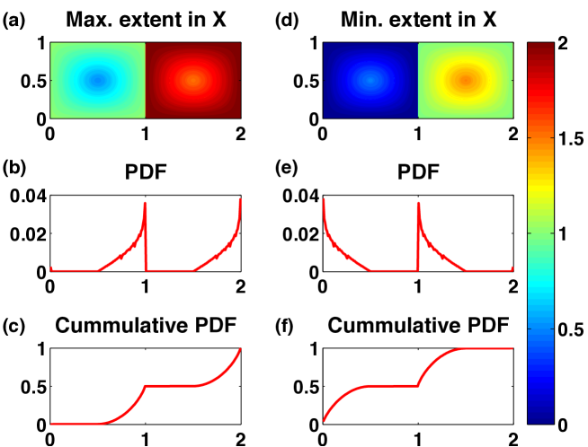
Figure 1: Two stationary coherent structures: the maximal (left) and minimal (right) $x$ position ($M^{\pm}_{\bf(1,0)}$) of all initial conditions is plotted (top), as are the corresponding PDF (middle) and CDF (bottom) functions. Each gyre appears in the PDF and correspondingly in the CDF: the left gyre accumulates to occupy exactly half of the domain, as apparent from the plateau region. The centers and extents of the two gyres are clearly seen. Eq. 8, $A=0.25,\epsilon=0$ and $\tau=200$.

We propose that by monitoring these fields, which are trivial to compute, we can infer quite a few properties of the Lagrangian flow structure both asymptotically and transiently. Moreover, we propose that such properties may be found quite efficiently by analyzing the cumulative distribution function (CDF) of the MET field. This may lead to significant data reduction from 2D fields maps (e.g. of the FTLE or RD) to a 1D plot. Often, especially in realistic geophysical applications, the amount of data (e.g. data extracted from satellites or from general circulation models) is huge and time-dependent, and efficient data-compression methods are needed. As described in the next section, the shape of the CDF provides information about the existence of coherent structures, their locations, and the existence of chaotic zones. It seems that some of the properties may even be inferred from a sampling of the flow field in only a few directions, making this diagnostic a potentially useful tool in real applications allowing a limited sampling of the flow (e.g., by only few drifters) even in the fully three dimensional setting. We will further explore this direction in future studies.

III Typical features of the MET-Toy models

Next we examine the properties of the extremal fields at typical structures that appear in unsteady flows. To this aim we first consider prototypical models for stirring and mixing in bounded domains - the steady and time-dependent double gyre models. We then consider the oscillating vortex pair model to demonstrate the method on a flow in an unbounded domain.

A CS, loosely defined as a group of trajectories with a common averaged behavior on some fast eddy-turnover time scale, may be stationary, gently oscillating, rotating or advected in an unbounded domain. The FTLE field for particles in all such structures asymptotically vanishes. Below, we list the characteristic features of the MET in these different settings. We show that while the MET is simpler to compute it provides additional information about the properties of the coherent structures. To gain intuition we examine the double gyre model Shadden et al. (2005):

$$\Psi_{xy}(x,y,t) = A\sin(\pi f(x,t))\sin\pi y$$ (8)

$$f\left(x,t\right) = \epsilon\sin\omega t\ x^{2}+(1-2\epsilon\sin\omega t)x.\$$

We begin with the trivial case of the steady double gyre ($\epsilon=0)$ and then continue to more realistic settings.

A single stationary coherent structure. Consider the stationary double gyre model. The maximal and minimal extents in the $x$ direction for this case are shown in Fig. 1a,d. The flow has two symmetric gyres lying along the horizontal direction and no mixing zone. Examine the left gyre first. All trajectories belonging to the left gyre are bounded and periodic in time. Hence, for any fixed $t_{1}$, for all $\tau$, $M_{\bf r}(\tau;x_{0},t_{1})$ and $M^{\pm}_{\bf r}(\cdot)$ are finite and, for sufficiently large $\tau$, $M_{\bf r}(\cdot)$ is equal to the width of the periodic orbit in the direction $\mathbf{r}$, whereas $M^{\pm}_{\bf r}$ provide the maximal and minimal extents in this direction.

Asymptotic form of the PDF and CDF The PDFs and CDFs for this case are also shown in Fig. 1. The CDF of $M^{+}_{\bf r}$ converges to a piecewise smooth increasing function which starts increasing quadratically from zero concentration at the coherent structure center $(x=0.5)$ and abruptly stops increasing at the coherent structure boundary ($x=1.0)$. The CDF of $M^{-}_{\bf r}$ (Fig. 1f) starts increasing abruptly at the coherent structure leftmost boundary $(x=0)$ and stops increasing quadratically at the coherent structure center ($x=0.5)$. The area fraction of the left coherent structure is the CDF value at the plateau.

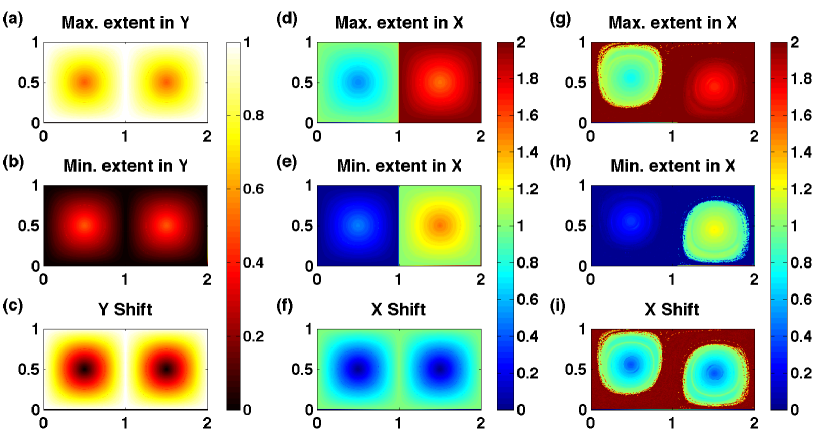
Figure 2: Two stationary (a-f) and oscillatory (g-i) coherent structures. a-c) The need to choose resolving direction for obtaining the number of distinct CSs from the corresponding CDFs is demonstrated. The two gyres here have exactly the same extent in the $y$ direction (i.e. identical $M^{\pm}_{\bf(0,1)}$ values) hence the CDF of the $M^{\pm}_{\bf(0,1)}$ does not lead to a distinction between the left and right gyres. d-f) The need for the maximal/minimal quantifiers is demonstrated - while the maximal/minimal $x$ values ($M^{\pm}_{\bf(1,0)}$) distinguish between the right and left gyres, their difference, the maximal shift $M_{\bf(1,0)}$, does not. g-i) The applicability to unsteady flow is demonstrated (Eq. 8 with $A=\epsilon=0.25,\omega=2\pi/10$ and $\tau=200$). Notice that in both the stationary and oscillatory cases, at the coherent structure centers the fields $M_{\mathbf{r}},M^{+}_{\mathbf{r}},-M^{-}_{\mathbf{r}}$ attain their local minima. In the stationary case (a-f) the value of $M^{\pm}_{\mathbf{r}}$ at the center matches the center position whereas in the oscillatory case there is a mismatch due to the oscillation: $M^{\pm}_{\mathbf{r}}-x_{c}(t_{0};t_{0})\cdot\mathbf{r}\neq 0.$

Several stationary coherent structures. The need for the three quantifiers $M_{\bf r},M^{\pm}_{\bf r}$ and the directional dependence is clarified when several coherent structures coexist in the flow. Fig. 2 shows these three fields for two directions ($x$ and $y$). First, we observe that the $M_{\mathbf{r}}^{\pm}$ fields distinguish between different CSs provided that the structures have no overlap in the direction $\mathbf{r}$. In our example it is clear that the $x$ maximal/minimal extent fields ($M_{\mathbf{(1,0)}}^{\pm}$, Figs. 1 and 2d,e) distinguish between the left and right gyres whereas the $y$ maximal/minimal extent fields ($M_{\mathbf{(0,1)}}^{\pm}$, Fig. 2g,h) do not. More generally, denote by $L_{x-left}$ the $x$ coordinate of the right boundary of the left gyre, by $(C_{x-right},C_{y-right})$ the center of the right gyre and by $L_{y}$ the height of the gyres. Then, for $\mathbf{r}=(r_{x},r_{y})$, we see that $M_{\mathbf{r}}^{+}(\text{i.c. in left gyre})=\max_{\text{i.c. in left gyre}}(x(t)r_{x}+y(t)r_{y})<L_{x-left}r_{x}+L_{y}r_{y}$ whereas $M_{\mathbf{r}}^{+}(\text{i.c. right gyre})=\max_{\text{i.c. in right gyre}}(x(t)r_{x}+yr_{y})>C_{x-right}r_{x}+C_{y-right}r_{y}$. Hence, if there is a gap between the two bounds (here $\frac{r_{y}}{r_{x}}<\frac{C_{x-right}-L_{x-left}}{L_{y}-C_{y-right}}$ ) we will call r a resolving direction and then the CDFs of $M_{\mathbf{r}}^{\pm}$ show two distinct monotone increasing regimes each corresponding to a different gyre as in Fig. 1. On the other hand, we notice that the $M_{\bf r}$ field is identical for the two gyres, and more generally, for all r, all the coherent structures are lumped together in this field (similarly to the FTLE and RD fields).

More generally, we see that depending on the structures’ alignments, a direction $\mathbf{r}$ may or may not resolve the structures. If the center of one structure is bounded away from the maximal (or minimal) extent of the other in the direction $\mathbf{r}$ we do have separation - a gap in the $M_{\mathbf{r}}^{\pm}$ values. We expect to be able to find such resolving directions when there is a small number of coherent structures, but not when there are many possibly disordered structures in the domain (as in 2D-turbulent flows), see discussion.

The important conclusion from the above is that the CDF of the $M_{\mathbf{r}}^{\pm}$ fields with a resolving direction r may be used to distinguish between the existence of multiple vs. a single CSs (thus helping in data reduction). In contrast, the CDF of the $M_{\mathbf{r}}$ field, of the MET in non resolving directions, of the FTLE field and of other similar fields cannot help in counting the number of distinct CSs.

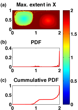
Figure 3: Oscillatory double gyre - the maximal extent in $x$, $M^{+}_{\bf(1,0)}$, its PDF, CDF and the mixing layer. The two gyres and the mixing layer are clearly distinguishable in the CDF, whereas in the PDF the high concentration of the distribution function in the mixing layer bin ($x_{max}\lesssim 2$) makes the contributions to the regular coherent structures nonvisible. $A=\epsilon=0.25,\omega=2\pi/10$ and $\tau=200$.

Oscillating coherent structures and the mixing layer Consider now the periodically perturbed double gyre model shown in Fig. 2g-i. Here, trajectories starting inside the two gyres move on some invariant rings around the two oscillating centers located near $x=0.5,1.5,y=0.5$. We expect that most of the initial conditions in these gyres belong to KAM tori, namely they perform regular (quasiperiodic) motion. We observe that the properties of the fields $M_{\mathbf{r}},M^{\pm}_{\mathbf{r}}$ and their CDFs in the CSs are similar to those of the steady gyres (Fig. 3). To gain intuition, assume that the trajectories are of the form: $x(t;t_{0})=x_{c}(t;t_{0})+g(t;x_{0})$ where $x_{c}(t;t_{0})$ is some unknown slowly moving center and $g$ is rapidly oscillating with zero mean (otherwise the particle drifts away from the center). The main difference between these and the stationary CSs, and in fact a way to identify these oscillating structures, appears when one examines the value of $M_{\mathbf{r}}^{\pm}$ at the coherent structure center $x_{c}(t;t_{0})$, where, as before, we may define $x_{c}(t_{0};t_{0})$ as the trajectory along which $M_{\mathbf{r}}$ attains its local minima. In the steady case, we have $M_{\mathbf{r}}^{-}=M_{\mathbf{r}}^{+}=x_{c}(t_{0};t_{0})\cdot\mathbf{r}$, whereas in the oscillating case these values provide the minimal and maximal central location of the coherent structure along the $\mathbf{r}$ direction, see Fig. 2g-i (see also Fig. 4).

In the oscillatory case a mixing layer appears: it consists of chaotic trajectories having sensitive dependence on i.c. that eventually encircle both gyres. Hence, for all i.c.’s $x_{0}$ in the mixing layer, the values of $M_{\bf r},M^{\pm}_{\bf r}$ asymptote to the width/the extent of the mixing layer in the $\mathbf{r}$ direction. Hence, the PDFs of $M_{\bf r},M^{\pm}_{\bf r}$ converge to a delta function on the chaotic component, at the value of the maximal extent of the mixing layer (in the present case the maximal extent of the domain) - the chaotic bin. In the PDF of these fields the only observable structure is the mixing layer whereas the regular coherent structures become invisible (Fig. 3b). In the CDF plot the finite volume of the chaotic layer is apparent (Fig. 3c).

The boundary between the mixing layer and the coherent structure is especially interesting - the MET are discontinuous at this boundary (Fig. 3,4,5). Moreover, the convergence characteristics of these fields are different in the mixing vs. the CS regions. High variability is expected in the chaotic zone whereas in the coherent structures the convergence is expected to be regular.

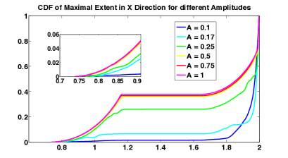
Figure 4: Oscillatory double gyre for different base flow intensity $A$ after 20 periods. Left: The CDF provides succinct presentation of the CS size and location for the different flows without using any flow visualization analysis. Right: The maximal extent in $x$, $M^{+}_{\bf(1,0)}$, is shown for four different base flow strengths. The two gyres and the mixing layer are clearly distinguishable. The difference between the location of the gyre center and its maximal value provides information regarding its oscillation magnitude. The accumulated size of the coherent structures is seen to decrease here with decreasing $A$ thus providing estimates for the area of the mixing zone. $\epsilon=0.25,\omega=2\pi/10$ and $\tau=200$.

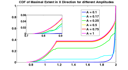
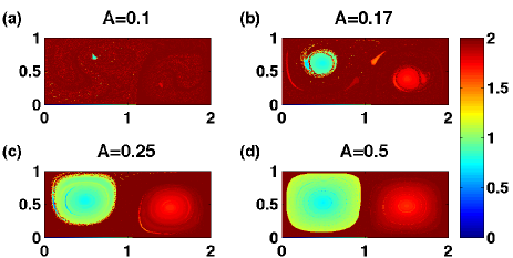
Figure 5: Oscillatory double gyre for different base flow intensity $A,$ as in Fig 4 for double the integration time (40 periods). The convergence of the CDFs and of the MET fields in regular regions is mainly achieved already after 20 periods, whereas the mixing layers have slower convergence and do not achieve their asymptotic behavior even after 40 periods. $\epsilon=0.25,\omega=2\pi/10$ and $\tau=400$.

Finally, Figs. 4 and 5 show that the CDFs of the MET fields provide a succinct way to compare the mixing properties of different flow fields. In these figures we compare the CDFs of the unsteady double gyre model for decreasing power of the gyre intensity after 20 (Fig. 4) and 40 (Fig. 5) periods. By decreasing the gyre intensity ($A$ in Eq. 8) we effectively increase the non-dimensional period of the oscillatory component Rom-Kedar and Poje (1999). The CDFs reveal how the two CSs centers oscillate to larger extent and shrink in size with $A$ without using any flow visualization analysis. Indeed, notice that the parabolic increase in the CDF starting near $x=0.7$ ($x=1.7)$ corresponds to the maximal $x$-locations of the left (right) CS center respectively. Thus, the change in this value with $A$ (see insert) indicates that the centers experience larger oscillations as $A$ decreases. The plateau value of the CDF provides the area of the left CS (seen to decrease from 0.4 to nearly vanishing values as $A$ decreases). The sharp increase in the CDF towards $x=2.0$ indicates the transition to the mixing layer orbits, thus, for sufficiently large $\tau$, the value of the CDF at the transition point provides the total area of the regular component. Notice that when $A$ decreases to $0.17$ the two gyres break into smaller CSs, some of these begin to rotate in the box (see the bright red crescent on the left part of the box - this crescent together with the island to the right of the center line correspond to a period two CS. The large discrepancy between the location of this crescent and the $M^{+}_{\bf(1,0)}$ value in it, which is equal to that found in the other island suggests its rotational nature. This may be verified by trajectory computations and by looking at the minimal extent field, not shown). The above observations apply to a sufficiently long extremal window $\tau$. Comparing Figs. 4 and 5 it is seen that while the CDF component of the CSs appears to converge already after 20 periods the mixing component has not reached its asymptotic form even after 40 cycles. Indeed, the ghost of the stable manifold is readily seen for short extremal windows. These distinct convergence properties and the transient features of the MET may be utilized to distinguish between different regions and for locating dividing surfaces - this is left to future studies.

CS in unbounded flows Next we consider an open flow model, the Oscillating Vortex Pair (OVP): a vortex pair in an oscillating strain-rate field embedded in a uniform flow. The non-dimensional stream function Rom-Kedar et al. (1990) is of the form :

$$\psi(x,y,t) = -\log\frac{(x-x_{v})^{2}+(y-y_{v})^{2}}{(x-x_{v})^{2}+(y+y_{v})^{2}}-vy+\epsilon xy\sin(\omega t)$$

$$\frac{dx_{v}}{dt} = \frac{1}{2y_{v}}-v+\epsilon x_{v}\sin(\omega t),$$ (9)

$$\frac{dy_{v}}{dt} = -\epsilon y_{v}\sin(\omega t)$$

where $(x_{v}(t),\pm y_{v}(t))$ denotes the vortex locations and $x_{v}(0)=0,y_{v}(0)=1$. The vortex pair moves, in an oscillatory fashion, in the positive $x$ direction with an average horizontal velocity $v_{vort}=0.5-v+O(\epsilon)$. As the vortex pair advects it carries with it a body of fluid, and due to the oscillations it sheds parts of this body of fluid in the form of lobes, see Rom-Kedar et al. (1990). There, $v$ was tuned so that $v_{vort}\approx 0$ and thus the mixing was observed in the vortex pair moving frame. Here we take different values of $v$ to examine the dependence of the MET methodology on the frame of reference .

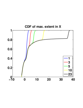
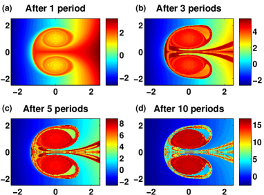
Figure 6: The MET for the OVP open flow - dependence on time. The four right panels show the maximal extent in $x$, $M^{+}_{\bf(1,0)}$, at four different extremal windows ($\tau=(1,3,5,10)\cdot 2\pi/\omega$) for the OVP flow ( Eq. 9 with $\epsilon=0.2,\omega=1.45,v=0.25$). The left panel shows the CDF of this flow at the corresponding times - the rightmost curve after 23 periods. The location and size of the vortical core may be easily identified from the CDF.

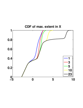
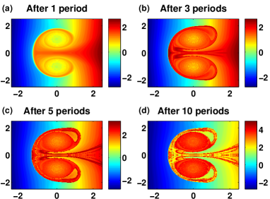
Figure 7: The MET dependence on frame of reference. The OVP flow with the same parameters as in Fig. 6 yet in a different moving frame (Eq. 9 with $\epsilon=0.2,\omega=1.45$ and $v=0.5$ ). Comparing the right panels here with those of Fig. 6 we observe that similar structures appear and the main change is in the color bar. Indeed, the left panel showing the CDF of the slower moving frame shows that after the initial transition the frame of reference only shifts the location of the CS, as expected.

Fig. 6 shows the maximal extent in $x$ and the associated CDFs of the OVP flow at several extremal windows of increasing length. The CSs appear as a sharp parabolic increase in the CDF, its center moving with time. Thus it is possible to detect the area and location of the body of fluid which advects with the vortices as well as to identify the volume of fluid that is shed by the lobes.

Fig. 7 shows, as in Fig. 6, the maximal extent in $x$ of the OVP flow, but in a different moving frame. After some time, aside of the change in the color bar, similar structures as in Fig. 6 appear, as is also apparent from the CDFs of the two simulations. Thus, it is demonstrated that for sufficiently large $\tau$ the MET is frame-independent Poje and Haller (1999); Haller and Beron-Vera (2013) and applicable even when the structure moves out of the original region in which the particles are seeded. Note that these features are especially relevant to geophysical applications in which the observed domain is open and there is an unknown underlying current, see section IV.

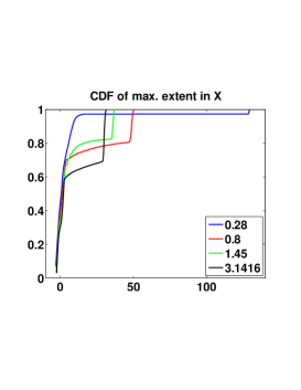
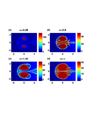
Figure 8: CSs dependence on parameters. On the right panels the maximal extent in $x$, $M^{+}_{\bf(1,0)}$, is shown for four different frequencies at $\tau=100$ (about 5, 12, 23 and 50 cycles of the corresponding frequencies). The left panel shows the CDF of these fields - the area and location of the CSs is easily extracted from the CDFs. Notice the non monotonic dependence of the core area on $\omega$.

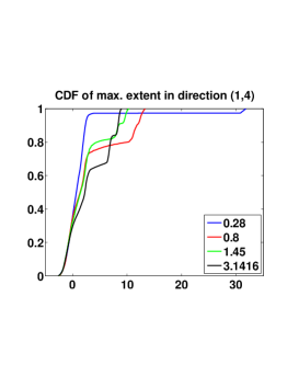
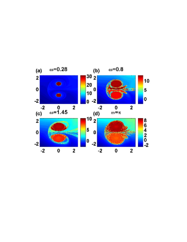
Figure 9: CSs in a resolving direction. On the right panel the maximal extent in $x+4y$, $M^{+}_{\bf(1,4)}$, is shown for four different frequencies (as in Fig. 8). The left panel shows the CDF of these fields. Here, the resolving direction distinguishes between the lower and upper vortex areas.

Fig. 8 (respectively 9) shows the maximal extent in $x$ (respectively in direction r=$(1,4)$) of the OVP flow for different frequencies of the strain field oscillations. The CSs area has a strong non monotonic dependence on the frequency (see also Rom-Kedar and Poje (1999)), as is apparent from both the CDF diagram and the extremal field plots. While the $x$ direction lumps together both vortices, the $(1,4)$ direction resolves the two structures.

Finally, Fig. 10 shows several other quantifiers to be compared with the maximal extent in $x$. Fig. 10 a (b) presents the traditional relative (absolute) dispersion fields and Fig. 10c (d) presents the maximal shift in $x$ ($y$). Since some of the particles move to the right (the vortex core region) and some to the left (the outer particles), the maximal shift in $x$ field together with the maximal extent field provide information on the directional motion of the particles. The maximal shift in $y$ (d) and the absolute dispersion (AD) field (b) provide similar division to core regions, mixing region and outer flow, yet these do not include directional information. The RD field (and similarly the FTLE) nicely detects the stable manifold, yet has similar, close to zero values everywhere else.

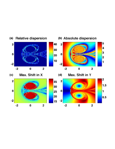
Figure 10: Different quantifiers for the OVP flow. a) The relative dispersion. b) The absolute dispersion c) The maximal shift in $x$, $M_{\bf(1,0)}$, d) The maximal shift in $y$, $M_{\bf(0,1)}$. Compare with Figs 8,9c in which the same flow is presented with the max. extent plots (Eq. 9 with $\epsilon=0.2,\omega=1.45,$ $v=0.25$ at $\tau=100$, i.e. after about 23 cycles).

It is worth pointing out the differences between moving CS and CS that has on average a zero displacement. To gain intuition, again assume that trajectories belonging to a CS which moves in an unbounded region along a direction r have the form $x(t;t_{0})=x_{c}(t;t_{0})+g(t;x_{0})$ where $x_{c}(t;t_{0})$ is the CS center, so $x_{c}(t;t_{0})\cdot\mathbf{r}$ is slowly increasing on average, and the rapidly oscillating $g$ has average zero. Then, while $M_{\mathbf{r}},M_{\mathbf{r}}^{+}$ may be unbounded in time, $M_{\mathbf{r}}$ and $M_{\mathbf{r}}^{+}$ still attain their local minima at $x_{c}$, see Figs. 6-10. On the other hand, in this case $M_{\mathbf{r}}^{-}$ contains very little information with regard to the CS - basically the launching point of the trajectories. If one chooses a direction which is perpendicular to the direction of motion (i.e. $y$ direction here), the number of separate regions may be detected, but the information on the CS motion is lost.

Trajectories that are far from the vortices experience, on average, a nearly uniform flow, hence the MET have a nice smooth dependence on initial conditions in such regions. The CDFs thus have a bulk smooth region corresponding to the background flow, a quadratically increasing portion with a moving center that corresponds to the CS, and some shedding of lobes that appear as small steps in the CDF, see Figs. 6-8. The speed and size of the moving CS can be thus easily determined from the CDF. Notice that the CS area is the relative fraction obtained from the CDF multiplied by the chosen seeding area (see below).

IV Real data

We next apply the MET analysis to real data from the eastern Mediterranean, using surface currents obtained from the AVISO database (http://www.aviso.oceanobs.com). Within this velocity field we deploy 10,000 virtual particles on an approximately 2 km grid and track them for 40 consecutive days. The particles are seeded in a much smaller domain than the domain covered by the altimeter so that even when they leave the initial seeding region their trajectories can still be computed, see Fig. 11 (transport properties in this region during this period were studied in Efrati et al. (2013)). During the period examined in this study, the distributed global product was a combination of altimetric data from Jason-1 and -2 and Envisat missions. The dataset is comprised of daily near-real-time sea-level-anomaly data files, gridded on a $\frac{1}{8}^{o}\times\frac{1}{8}^{o}$ Mercator grid. The methodology for extracting a velocity field from sea level data is known to introduce errors, as does the linear interpolation scheme we use for integrating trajectories. Other sources of uncertainties in the data are due to tides and atmospheric conditions. In particular, the extracted velocity field is not area-preserving. Although in stratified ocean the flow is approximately 2D (i.e. vertical velocities are few orders of magnitude smaller than the horizontal velocities), 3D effects may qualitatively changes surface mixing Aharon et al. (2012). Additionally, close to the coast, the use of satellite altimetry is known to be unreliable, so the dataset does not include measurements at distances of less than 10 km from the coastline. Despite these above-mentioned errors and limitations, our analysis seems to capture the existing CSs.

Since we do not have apriori knowledge of the flow field, we calculated both minimal and maximal extents along both the zonal (longitudinal) and meridional (latitudinal) directions for a few extremal time windows. The maximal extent in the latitudinal direction provided the best separation between the two complete CSs (centered at $35^{o}$ and $35^{o}50^{{}^{\prime}}$ north) that were detected in essentially all measures (see Figs. 12-14). The white area in these plots corresponds to trajectories that either originated or reached domains with no reliable velocity data by the end of the extremal window integration time (either approached the coastal area or left the region depicted in Fig. 11).

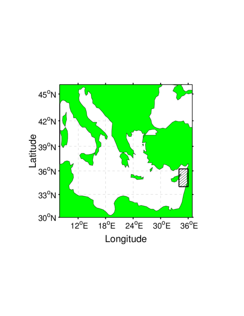
Figure 11: The eastern Mediterranean sea region in which particles are seeded (dashed rectangle) is contained in a large region where velocity data is available.

Fig. 12 shows the maximal extent in the latitudinal direction for three 10 days extremal time windows starting on Aug. 18, Sep. 6, and Sep. 16 (the Aug. 28 panel, not shown, is very similar to that of Sep. 6).

Fig. 13a,b shows the PDF and CDF of the maximal extent in the latitudinal direction for the middle extremal time window (Sep. 6-16). The CDF scale is multiplied by the approximate seeding area to obtain realistic information regarding the gyres size. Three distinct structures are clearly seen. The two CSs that are fully contained in the region (centered at $35^{o}$ and $35^{o}50^{{}^{\prime}}$ north) are manifested in the PDF and CDF with the typical asymmetric form, similar to Figs. 3-5. On the other hand the structure that is only partially contained in the domain in its south-west corner cannot be identified as a CS in the CDF. This suggests that we are seeing only a part of the CS or of another structure - to be resolved, a larger domain is needed. Fig  13c shows the CDF of the maximal extent in the latitudinal direction for four subsequent 10 days extremal time windows.

From the CDF plots it is seen that the main CS, centered near latitude $35^{o}$, keeps its latitude and size for the first 30 days, and then, in the last 10 days it shifts a bit north-word and a substantial part of its outer layer approaches the coastal area. The smaller northern CS, centered originally near latitude $35^{o}50^{{}^{\prime}}$ north, is seen to travel north-word right from the start (e.g. notice its color change between Fig. 12a and Fig. 12b ) and in the last 10 days most of the trajectories in it approached the coastline.

Fig. 14 shows a few more fields that provide additional information on the CS structure and demonstrate the importance of the choice of a resolving direction. Fig. 14a shows the maximal latitudinal shift, Fig. 14b,c show the maximal longitudinal shift and extent and Fig. 14d,e show the standard absolute and relative dispersion fields. In all these figures the two complete CSs are nicely seen. However, since the two gyres have overlapping field values (have the same color in the colormap), a PDF and CDF of any of the five presented fields will not exhibit the separate structures as seen in Fig. 13 for the resolving direction (here latitude). Of course, one can use a spatial fraction of the domain to isolate each of the gyres, and these specific plots also provide additional information regarding the longitudinal motion. Notice also that the RD field is more expensive computationally than any of the MET characteristics, and its computation in different time windows requires reseeding of particles (whereas all other computations are done by processing a single 40-days integration of the trajectories).

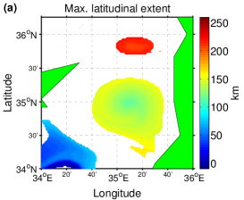
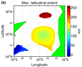
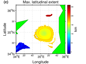
Figure 12: The maximal latitudinal extent ($M^{+}_{\bf(0,1)}$) of particles seeded on 18 of Aug. 2011 in the eastern Mediterranean sea. Three separate CSs are identified. Extremal windows of 10 days each are shown a) Aug. 18-Aug. 28 b) Sep. 6-Sep. 16 c) Sep. 16-Sep. 26. White regions correspond to trajectories which either originated or reached domains with no reliable velocity data (either approached the coastal area or left the region depicted in Fig. 11).

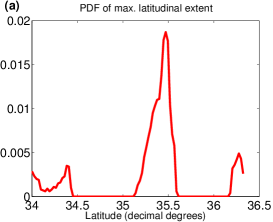
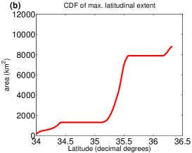
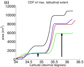
Figure 13: The PDF (a) and CDF (b) of the maximal latitudinal extent ($M^{+}_{\bf(0,1)}$) of particles seeded on 18 of Aug. 2011 for the extremal window Sep. 6-Sep. 16 (Fig 12b). The three distinct regions are clearly seen in the figures. The signature of the two CS which are fully contained in the region are similar to those appearing in the toy models. (c) shows the CDF for four 10-days periods: Aug. 18-28, Aug. 28-Sep. 6, Sep. 6-16, Sep. 16-26. Notice the changes in the CSs centers’ latitudes, the disappearance of the upper gyre and the dramatic decrease in the main gyre area - the gap between the two plateaus indicated by the arrows.

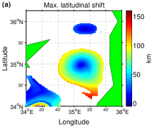
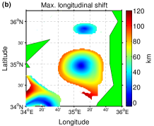
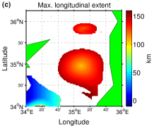
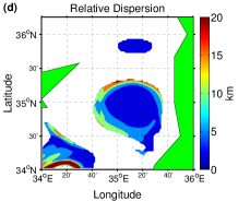
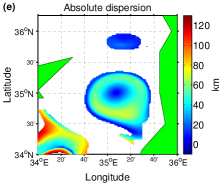
Figure 14: Other measures for the particles seeded on 18 of Aug. 2011 on the extremal window Aug. 18-Aug. 28. a) The maximal latitudinal shift ($M_{\bf(0,1)}$) b) The maximal longitudinal shift ($M_{\bf(1,0)}$) c) The maximal longitudinal extent d) the absolute dispersion e) the relative dispersion.

V Discussion

Our main result is the introduction of a new family of Lagrangian diagnostics, in particular the MET, and the demonstration that the CDF of the MET allows one to find important characteristics of the CSs at low computational cost. In particular, the number, location, and size of the coherent structures (nested sets of a continuum of ergodic components) with a volume above a threshold value may be found with no need for minimization or image processing procedures. A major advantage is thus the ability to compress a large amount of data into a simple diagnostic plot.

The signature of a CS in the CDF appears as a smooth curved increasing segment - the base of it and the value where it flattens or abruptly increases provide information on its spatial location and width along the specific direction that is used to compute the MET. The height difference between these values provides its area. The signature of a mixing layer (in closed domains) is a fast growing segment that asymptotes as $\tau$, the extremal window, grows to infinity, to a discontinuity of the CDF. A motion of the CS corresponds to a shift of its corresponding segment in the CDF with hardly any change of its shape. We demonstrated that the MET provides insightful information using toy models in both closed and open domains and on a real data set from the eastern Mediterranean Sea.

The MET and many other Lagrangian quantifiers (such as RD, FTLE, the hypergraph map and other averaged quantifiers Budišić et al. (2012); Mezic et al. (2010); Rypina et al. (2011); BozorgMagham et al. (2013); Shadden et al. (2005); Haller and Yuan (2000)) have a common feature: asymptotically these converge to constants on ergodic sets and hence, in principle, may be utilized to divide the phase space to separate ergodic components. In many applications, the transient properties of these and other Lagrangian quantifiers were studied, showing that in some cases ridges of finite time realizations of these fields provide good predictors for dividing surfaces. We expect that similar analysis can also be applied to finite time realizations of extremal fields (see especially Figs. 4 and 6) and this direction has yet to be explored. Here we exploit the asymptotic features of these fields as a way to identify CS. In this aspect, we note that the RD and FTLE are degenerate - they asymptote to zero in the regular regime and to a positive constant in the mixing zone. On the other hand, the value of the MET (and of the hypergraph map and other Lagrangian averages Mezic et al. (2010)) asymptotes to a smooth function in a regular region and to a constant in the chaotic zone. The unique feature of the MET is that if the direction r is resolving, its CDF readily provides additional information on the location and number of CSs (whereas with the other quantifiers the CDF lumps together all coherent structures).

Another distinguishing characteristic of the MET is that the convergence to its asymptotic value is always monotone in time whereas in all the other quantifiers convergence to their asymptotic values is oscillatory (except the arc-length map Mendoza and Mancho (2010); Alvaro de la et al. (2013) which is monotone yet unbounded). Hence we expect that the convergence of the MET will be faster and more regular. In fact, the temporal convergence properties of the MET may be related to the universal convergence associated with extreme value statistics of ergodic dynamical systems Collet (2001); Holland et al. (2012); Lucarini et al. (2012); Freitas and Freitas (2008); Freitas (2013). The implications of these on the convergence of the CDF, on the spatial smoothness of the MET, and on the sensitivity of these to noise and velocity errors have yet to be investigated.

The current work leaves many additional directions to be explored in future studies, including: (1) The transient MET fields in the coherent structures are quite smooth whereas their transient behavior in the mixing layers is noisy. This property may be utilized to distinguish between these regions on short time scales. More generally, the study of the transient behaviour of the MET in $\tau,t_{1}$ may reveal the structure (e.g. local dimension Lucarini et al. (2012); Rypina et al. (2011)) of the ergodic component. Possibly, it may reveal other transient transport processes, such as dividing surfaces (LCS) and the lobe structure Aharon (2009). (2) The applications shown here suggest that additional insight may be obtained by studying the temporal and spatial dependence of extreme values of other observable functions in systems with mixed phase space (e.g. velocities, speed, distance from the origin, stretching rates, strain rates, FTLE, recurrences Lucarini et al. (2012) etc.) (3) The study of open flows needs to be further explored. For open flows with moving CSs the difference between the traditional AD field and the MET fields is not dramatic, yet the MET fields provide the additional advantage of directional information and non-oscillatory convergence. (4) In real applications we often have a limited sampling of the flow along specific directions, e.g. by few drifters. How much of the flow characteristics can be extracted from such limited information is unclear. Based on our preliminary results (not shown), 1D sections might suffice to provide many of the flow characteristics. Moreover, this approach may work in higher dimensions as well. (5) In flows with a large number of CSs of different scales and locations, such as 2D-turbulent flows, it may become difficult to find resolving directions. In such cases it may be beneficial to adopt a multi scale strategy by which resolving directions are sought on subdomains. (6) Finally, we note that many of the above issues may be studied first on chaotic maps with mixed phase space behavior (e.g. we currently study the standard map and its higher dimensional extensions). Such studies allow the introduction of a more rigorous mathematical analysis.

In conclusion, we present new, promising Lagrangian diagnostics that enable the extraction of properties of coherent structures from large data sets by looking at extremal values of observables, their PDFs, and CDFs. These diagnostics are not only simple, intuitive, and computationally cheap; they also enable a significant data reduction, since it is possible to extract from the cumulative distribution functions much of the relevant information regarding the existence, location, size and motion of the coherent structures.

References

- Gawarkiewicz et al. (2007) G. Gawarkiewicz, S. Monismith, and J. Largier, Oceanography 20, 40 (2007).
- BozorgMagham et al. (2013) A. E. BozorgMagham, S. D. Ross, and D. G. Schmale III, Physica D (2013).
- Mezic et al. (2010) I. Mezic, S. Loire, V. A. Fonoberov, and P. Hogan, Science 330, 486 (2010).
- Olascoaga and Haller (2012) M. J. Olascoaga and G. Haller, Proceedings of the national academy of sciences of the United States Of America 109, 4738 (2012).
- Peacock and Haller (2013) T. Peacock and G. Haller, Physics Today 66, 41 (2013).
- Melsom et al. (2012) A. Melsom, F. Counillon, J. H. LaCasce, and L. Bertino, Ocean Dyn. 62, 1245 (2012).
- D’ovidio et al. (2009) F. D’ovidio, J. Isern-Fontanet, C. Lopez, E. Hernandez-Garcia, and E. Garcia-Ladon, Deep-Sea Res. 56, 15 (2009).
- Mariano et al. (2002) A. J. Mariano, A. Griffa, T. M. Özgökmen, and E. Zambianchi, J. Atmos. Oceanic Tech. 19, 1114 (2002).
- Aref (2002) H. Aref, Phys. Fluids 14, 1315 (2002).
- Ottino (1989) J. Ottino, The Kinematics of Mixing: Stretching, Chaos, and Transport (Cambridge University Press, Cambridge, MA, 1989).
- Mancho et al. (2006) A. M. Mancho, D. Small, and S. Wiggins, Phys. Reports 437, 55 (2006).
- Beron-vera and Olascoaga (2009) F. J. Beron-vera and M. J. Olascoaga, J. Phys. Oceanogr. 39, 1743 (2009).
- Koshel and Prants (2006) K. V. Koshel and S. V. Prants, Physics-uspekhi 49, 1151 (2006).
- Peacock and Dabiri (2010) T. Peacock and J. Dabiri, Chaos 20 (2010).
- Bollt and Santitissadeekorn (2013) E. M. Bollt and N. Santitissadeekorn, Applied and Computational Measurable Dynamics, Mathematical modeling and computation (SIAM, 2013).
- Prants (2013) S. V. Prants, Physica Scripta 87 (2013).
- Budišić et al. (2012) M. Budišić, R. Mohr, and I. Mezić, Chaos 22, 047510 (2012).
- Poje and Haller (1999) A. C. Poje and G. Haller, J. Phys. Oceanogr. 29, 1649 (1999).
- Haller and Beron-Vera (2013) G. Haller and F. J. Beron-Vera, J. Fluid Mech. 731 (2013).
- Pierrehumbert (1994) R. Pierrehumbert, Chaos solitons and fractals 4, 1091 (1994).
- Lin et al. (2011) Z. Lin, J.-L. Thiffeault, and C. R. Doering, J. Fluid Mech. 675, 465 (2011).
- Lingevitch and Bernoff (1994) J. Lingevitch and A. Bernoff, J. Fluid Mech. 270, 219 (1994).
- Mathew et al. (2005) G. Mathew, I. Mezic, and L. Petzold, Physica D 211, 23 (2005).
- Beigie et al. (1991) D. Beigie, A. Leonard, and S. Wiggins, Phys. Fluids A 3, 1039 (1991).
- Rom-Kedar and Poje (1999) V. Rom-Kedar and A. Poje, Phys. Fluids 11, 2044 (1999).
- Haller and Yuan (2000) G. Haller and G. Yuan, Physica D 147, 352 (2000).
- Shadden et al. (2005) S. C. Shadden, F. Lekien, and J. E. Marsden, Physica D 212, 271 (2005).
- Orre et al. (2006) S. Orre, B. Gjevik, and J. H. LaCasce, Cont. Shelf Res. 26, 1360 (2006).
- Boffetta et al. (2001) G. Boffetta, G. Lacorata, G. Radaelli, and A. Vulpiani, Physica D 159, 58 (2001).
- Lipphardt et al. (2006) B. Lipphardt, D. Small, A. Kirwan, S. Wiggins, K. Ide, C. Grosch, and J. Paduan, J. Mar. Res. 64, 221 (2006).
- Okubo (1970) A. Okubo, Deep-Sea Res. 17, 445 (1970).
- Weiss (1991) J. Weiss, Physica D 48, 273 (1991).
- Rypina et al. (2011) I. Rypina, S. E. Scott, L. J. Pratt, and M. G. Brown, Nonlin. Processes Geophys. 18, 977 987 (2011).
- Mendoza and Mancho (2010) C. Mendoza and A. M. Mancho, Phys. Rev. Lett. 105, 038501 (2010).
- Alvaro de la et al. (2013) C. Alvaro de la, C. Mechoso, A. Mancho, E. Serrano, and K. Ide, J. Atmos. Sci. 70, 2982 3001 (2013).
- Rom-Kedar et al. (1990) V. Rom-Kedar, A. Leonard, and S. Wiggins, J. Fluid Mech. 214, 347 (1990).
- Dellnitz and Junge (1999) M. Dellnitz and O. Junge, SIAM Journal on Numerical Analysis 36, 491 (1999).
- Froyland et al. (2007) G. Froyland, K. Padberg, M. H. England, and A. M. Treguier, Phys. Rev. Lett. 98 (2007).
- Froyland and Padberg-Gehle (2012) G. Froyland and K. Padberg-Gehle, Physica D 241, 1612 (2012).
- Aharon (2009) R. Aharon, Master’s thesis, Weizmann Institute of Science, Rehovot, Israel (2009), available at: http://www.earth.huji.ac.il/data/File/gildor/Rotem_thesis.pdf.
- Aharon et al. (2012) R. Aharon, V.Rom-Kedar, and H. Gildor, Phys. Fluids 24, 056603 (2012).
- Collet (2001) P. Collet, Erg. Theory Dyn. Sys. 21, 401 (2001).
- Holland et al. (2012) M. P. Holland, R. Vitolo, P. Rabassa, A. E. Sterk, and H. W. Broer, Physica D 241, 497 (2012).
- Lucarini et al. (2012) V. Lucarini, D. Faranda, and J. Wouters, J. Stat. Phys. 147, 63 (2012).
- Freitas and Freitas (2008) A. C. M. Freitas and J. M. Freitas, Stat. Prob. Lett. 78, 1088 (2008).
- Freitas (2013) J. M. Freitas, Dyn. Sys. 28, 302 (2013).
- Efrati et al. (2013) S. Efrati, Y. Lehahn, E. Rahav, N. Kress, B. Herut, I. Gertman, R. Goldman, T. Ozer, M. Lazar, and E. Heifetz, Biogeosciences 10, 3349 (2013).