Comparison of POD reduced order strategies for the nonlinear 2D Shallow Water Equations

Abstract

This paper introduces tensorial calculus techniques in the framework of Proper Orthogonal Decomposition (POD) to reduce the computational complexity of the reduced nonlinear terms. The resulting method, named tensorial POD, can be applied to polynomial nonlinearities of any degree $p$. Such nonlinear terms have an on-line complexity of $\mathcal{O}(k^{p+1})$, where $k$ is the dimension of POD basis, and therefore is independent of full space dimension. However it is efficient only for quadratic nonlinear terms since for higher nonlinearities standard POD proves to be less time consuming once the POD basis dimension $k$ is increased. Numerical experiments are carried out with a two dimensional shallow water equation (SWE) test problem to compare the performance of tensorial POD, standard POD, and POD/Discrete Empirical Interpolation Method (DEIM). Numerical results show that tensorial POD decreases by $76\times$ times the computational cost of the on-line stage of standard POD for configurations using more than $300,000$ model variables. The tensorial POD SWE model was only $2-8\times$ slower than the POD/DEIM SWE model but the implementation effort is considerably increased. Tensorial calculus was again employed to construct a new algorithm allowing POD/DEIM shallow water equation model to compute its off-line stage faster than the standard and tensorial POD approaches.

Keywords— tensorial proper orthogonal decomposition; discrete empirical interpolation method; reduced-order modeling; shallow water equations; finite difference methods; Galerkin projections

1 Introduction

Modeling and simulation of multi-scale complex physical phenomena leads to large-scale systems of coupled partial differential equations, ordinary differential equations, and differential algebraic equations. The high dimensionality of these models poses important mathematical and computational challenges. A computationally feasible approach to simulate, control, and optimize such systems is to simplify the models by retaining only those state variables that are consistent with a particular phenomena of interest.

Reduced order modeling refers to the development of low-dimensional models that represent important characteristics of a high-dimensional or infinite dimensional dynamical system. The reduced order methods can be cast into three broad categories: Singular Values Decomposition (SVD) based methods, Krylov based methods and iterative methods combining aspects of both the SVD and Krylov methods (see e.g. Antoulas [3]).

For linear models, methods like balanced truncation (Moore [57], Antoulas [4], Sorensen and Antoulas [78], Mullis and Roberts [58]) and moment matching (Freund [28], Feldmann and Freund [27], Grimme [35]) have been proving successful in developing reduced order models. However, balanced truncation doesn’t extend easily for high-order systems, and several grammians approximations were proposed leading to methods such as approximate subspace iteration (Baker et al. [6]), least squares approximation (Hodel [41]), Krylov subspace methods (Jaimoukha and Kasenally [43] and Gudmundsson and Laub [36] ) and balanced Proper Orthogonal Decomposition (Willcox and Peraire [85]). Among moment matching methods we mention partial realization (Gragg and Lindquist [31], Benner and Sokolov [12]), Padé approximation (Gragg [30], Gallivan et al. [29], Gutknecht [38], Van Dooren [84]) and rational approximation (Bultheel and Moor [16]).

While for linear models we are able to produce input-independent highly accurate reduced models, in the case of general nonlinear systems, the transfer function approach is not yet applicable and input-specified semi-empirical methods are usually employed. Recently some encouraging research results using generalized transfer functions and generalized moment matching have been obtained by Benner and Breiten [11] for nonlinear model order reduction but future investigations are required.

Proper Orthogonal Decomposition and its variants are also known as Karhunen-Loève expansions [45, 53], principal component analysis Hotelling [42], and empirical orthogonal functions Lorenz [54] among others. It is the most prevalent basis selection method for nonlinear problems and, among other requirements, relies on the fact that the desired simulation is well simulated in the input collection. Data analysis using POD is conducted to extract basis functions, from experimental data or detailed simulations of high-dimensional systems (method of snapshots introduced by Sirovich [75, 76, 77]), for subsequent use in Galerkin projections that yield low dimensional dynamical models. Unfortunately the standard POD approach displays a major disadvantage since its nonlinear reduced terms still have to be evaluated on the original state space making the simulation of the reduced-order system too expensive. There exist several ways to avoid this problem such as the empirical interpolation method (EIM) Barrault et al. [7] and its discrete variant DEIM Chaturantabut [20], Chaturantabut and Sorensen [23, 22], best points interpolation method Nguyen et al. [60]. Missing point estimation Astrid et al. [5] and Gauss-Newton with approximated tensors Amsallem et al. [2], Carlberg and Farhat [17], Carlberg et al. [18, 19, 19] methods are relying upon the gappy POD technique Everson and Sirovich [25] and were developed for the same reason. Reduced basis methods have been recently developed and utilize on greedy algorithms to efficiently compute numerical solutions for parametrized applications Barrault et al. [7], Grepl and Patera [33], Patera and Rozza [63], Rozza et al. [70], Dihlmann and Haasdonk [24].

Dynamic mode decomposition is a relatively recent development in the field of modal decomposition (Rowley et al. [69], Schmid [74], Tissot et al. [82]) and in comparison with POD approximates the temporal dynamics by a high-degree polynomial. Trajectory piecewise linear method proposed by Rewieński and White [66] follows a different strategy where the nonlinear system is represented by a piecewise-linear system which then can be efficiently approached by the standard linear reduction method. Parameter model reduction has emerged recently as an important research direction and Benner et al. [13] highlights the major contribution in the field.

This paper combines standard POD and tensor calculus techniques to reduce the on-line computational complexity of the reduced nonlinear terms for a shallow water equations model. Tensor based calculus was already applied by Kunisch and Volkwein [48], Kunisch et al. [50] to represent quadratic nonlinearities of reduced order POD models. We show that the tensorial POD (TPOD) approach can be applied to polynomial nonlinearities of any degree $p$, and the its representation has a complexity of $\mathcal{O}(k^{p+1})$, where $k$ is the dimension of POD subspace. This complexity is independent of the full space dimension. For $k$ between $10$ and $50$ and $p=2$ the number of floating-point operations required to calculate the tensorial POD quadratic terms is $10$–$40\times$ lower than in the case of standard POD, and $10$–$20\times$ higher than for the POD/DEIM. However, CPU time for solving the TPOD SWE model (on-line stage) is only $2$–$8\times$ times slower than POD/DEIM SWE model for $10^{3}$–$10^{5}$ grid points, $k\leq 50$, and number of DEIM interpolation points $m\leq 180$. For example, for an integration interval of $3$h, $10^{5}$ mesh points, $k=50$, and $m=70$, tensorial POD and POD/DEIM are $76\times$ and $450\times$ faster than standard POD, but the implementation effort of POD/DEIM is considerably increased. Many useful models are characterized by quadratic nonlinearities in both fluid dynamics and geophysical fluid flows including SWE model. In the case of cubic or higher polynomial nonlinearities the advantage of tensorial POD is lost and its nonlinear computational complexity is similar or larger than the computational complexity of the standard POD approach. This proves that for models depending only on quadratic nonlinearities, the tensorial POD represents a solid alternative to POD/DEIM where the implementation effort is considerably larger. We also propose a fast algorithm to pre-compute the reduced order coefficients for polynomial nonlinearities of order $p$ which allows the POD/DEIM SWE model to to compute its off-line stage faster than the standard and tensorial POD approaches despite additional SVD calculations and reduced coefficients computations.

The paper is organized as follows. Section 2 reviews the reduced order modeling methodologies used in this work: standard, tensorial, and DEIM POD. Section 3 analyses the computational complexity of the reduced order polynomial nonlinearities for all three methods, and introduces a new DEIM based algorithm to efficiently compute the coefficients needed for reduced Jacobians. Section 4 discusses the shallow water equations model and its full implementation, and Section 5 describes the construction of reduced models. Results of extensive numerical experiments are discussed in Section 6 while conclusions are drawn in Section 7.

2 Reduced Order Modeling

For highly efficient flows simulations, reduced order modeling is a powerful tool for representing the dynamics of large-scale dynamical systems using only a smaller number of variables and reduced order basis functions. Three approaches will be considered in this study: standard Proper Orthogonal Decomposition (POD), tensorial POD (TPOD), and POD/Discrete Empirical Interpolation Method (POD/DEIM). They are discussed below. The tensorial POD approach proposed herein is different than the method of Belzen and Weiland [10] which makes use of tensor decompositions for generating POD bases.

2.1 Standard Proper Orthogonal Decomposition

Proper Orthogonal Decompositions has been used successfully in numerous applications such as compressible flow Rowley et al. [67], computational fluid dynamics Kunisch and Volkwein [49], Rowley [68], Willcox and Peraire [85], aerodynamics [15]. It can be thought of as a Galerkin approximation in the spatial variable built from functions corresponding to the solution of the physical system at specified time instances. Noack et al. [62] proposed a system reduction strategy for Galerkin models of fluid flows leading to dynamic models of lower order based on a partition in slow, dominant and fast modes. San and Iliescu [73] investigate several closure models for POD reduced order modeling of fluids flows and benchmarked against the fine resolution numerical simulation.

In what follows, we will only work with discrete inner products (Euclidian dot product) though continuous products may be employed too. Generally, an atmospheric or oceanic model is usually governed by the following semi–discrete dynamical system

$$\frac{d{\bf x}(t)}{dt}={\bf F}({\bf x},t),~{}~{}~{}~{}{\bf x}(0)={\bf x}_{0}\in\mathbb{R}^{n}.$$ (1)

From the temporal-spatial flow ${\bf x}(t)\in\mathbb{R}^{n}$, we select an ensemble of $N_{t}$ time instances ${\bf x}_{1},...,{\bf x}_{N_{t}}\in\mathbb{R}^{n},~{}n$ being the total number of discrete model variables per time step and $N_{t}\in\mathbb{N},~{}N_{t}>0$. Let us define the centering trajectory, shift mode, or mean field correction (Noack et al. [61]) ${\bf\bar{x}}=\frac{1}{N}_{t}\sum_{i=1}^{N_{t}}{\bf x}_{i}$. The method of POD consists in choosing a complete orthonormal basis $U=\{{\bf u}_{i}\},~{}i=1,..,k;~{}k>0;~{}u_{i}\in\mathbb{R}^{n};~{}U\in\mathbb{R}^{n\times k}$ such that the mean square error between ${\bf x}(t)$ and POD expansion ${\bf x}^{POD}(t)={\bf\bar{x}}+U{\bf\tilde{x}}(t),~{}{\bf\tilde{x}}(t)\in\mathbb{R}^{k}$ is minimized on average. The POD dimension $k\ll n$ is appropriately chosen to capture the dynamics of the flow as follows:

1:Calculate the mean ${\bf\bar{x}}=\frac{1}{N_{t}}\sum_{i=1}^{N_{t}}{\bf x}_{i}$.

2:Set up the correlation matrix $K=[k_{ij}]_{i,j=1,..,n}$ where $k_{ij}=\langle{\bf x}_{i}-{\bf\bar{x}},{\bf x}_{j}-{\bf\bar{x}}\rangle$, and $\langle\cdot,\cdot\rangle$ being the Euclidian dot product.

3:Compute the eigenvalues $\lambda_{1}\geq\lambda_{2}\geq...\lambda_{n}\geq 0$ and the corresponding orthogonal eigenvectors ${\bf v}^{1},{\bf v}^{2},..,{\bf v}^{n}\in\mathbb{R}^{n}$ of $K$.

4:Set ${\bf u}_{i}=\langle{\bf v}^{i},{\bf x}_{i}-{\bf\bar{x}}\rangle$, $i=1,..,n.$ Then, ${\bf u}_{i},~{}i=1,..,n$ are normalized to obtain an orthonormal basis.

5:Define $I(m)={\frac{\sum_{i=1}^{m}\lambda_{i}}{\sum_{i=1}^{n}\lambda_{i}}}$ and choose $k$ such that $k=\min\{I(m):I(m)\geq\gamma\}$ where $0\leq\gamma\leq 1$ is the percentage of total informations captured by the reduced space $\textrm{span}\{{\bf u}_{1},{\bf u}_{2},...,{\bf u}_{k}\}.$ Usually $\gamma$ is taken $0.99$.

Algorithm 1 POD basis construction

To obtain the reduced model of (1), we first employ a numerical scheme to solve the full model for a set of snapshots and follow the above procedure, then use a Petrov–Galerkin (PG) projection of the full model equations onto the space $\mathcal{X}^{k}$ spanned by the POD basis elements

$$\frac{d{\bf\tilde{x}}(t)}{dt}=W^{T}{\bf F}\bigg{(}{\bf\bar{x}}+U{\bf\tilde{x}}(t),t\bigg{)},~{}~{}~{}{\bf\tilde{x}}(0)=W^{T}\bigg{(}{\bf x}(0)-{\bf\bar{x}}\bigg{)},$$ (2)

where $W\in\mathbb{R}^{n\times k}$ contains the discrete test functions from the PG projection, i.e. $W^{T}U=I\in\mathbb{R}^{k}$. The Galerkin projection may be also a choice being just a particular case of PG ($W=U$).

The efficiency of the POD-Galerkin techniques is limited to linear or bilinear terms, since the projected nonlinear term at every discrete time step still depends on the number of variables of the full model:

$$\tilde{N}({\bf\tilde{x}})=\underbrace{W^{T}}_{k\times n}\underbrace{{\bf F}({\bar{\bf x}}+U{\bf\tilde{x}}(t))}_{n\times 1}.$$

To be precise, consider a steady polynomial nonlinearity $x^{p}$. A POD expansion involving mean ${\bf\bar{x}}$ will unnecessarily complicate the description of tensorial POD representation of a $p^{\rm th}$ order polynomial nonlinearity. Moreover the terms depending on ${\bf\bar{x}}$ are just a particular case of the term depending only on $U{\bf\tilde{x}}$ since vector componentwise multiplication is distributive over vector addition. Consequently the expansion ${\bf\bar{x}}\approx U{\bf\tilde{x}}$ will not decrease the generality of the reduced nonlinear term. In the finite difference case, the standard POD projection is described as follows

$$\tilde{N}({\bf\tilde{x}})=\underbrace{W^{T}}_{k\times n}\,\underbrace{\left(U{\bf\tilde{x}}\right)^{p}}_{n\times 1}$$ (3)

where vector powers are taken component-wise.

To mitigate this inefficiency we propose two approaches: (1) Tensorial POD and (2) Discrete Empirical Interpolation Method. The former approach is able to calculate the reduced polynomial nonlinearities independent of $n$, while the latter method can handle efficiently all type of nonlinearities.

2.2 Tensorial POD

Tensorial POD technique employs the simple structure of the polynomial nonlinearities to remove the dependence on the dimension of the original discretized system by manipulating the order of computing. It can be successfully used in a POD framework for finite difference (FD), finite element (FE) and finite volume (FV) discretization methods and all other type of discretization methods that engage in spectral expansions. Tensorial POD separates the full spatial variables from reduced variables allowing fast nonlinear terms computations in the on–line stage. For time dependent nonlinearities this implies separation of spatial variables from reduced time variables. Thus, the reduced nonlinear term evaluation requires a tensorial Frobenius dot-product computation between rank $p$ tensors, where $p$ is the order of polynomial nonlinearity. The projected spatial variables are stored into tensors and calculated off–line. These are also used for reduced Jacobian computation in the on-line stage.

The tensorial POD representation of (3) is given by vector

$${\bf\mathcal{M}}=\big{[}{\bf\mathcal{M}}^{i}\big{]}_{i=1,2,..,k};\quad{\bf\mathcal{M}}^{i}=\left\langle{\bf M}^{i},{\bf\tilde{X}}\right\rangle_{\textrm{Frobenius}}\in\mathbb{R},~{}i=1,2,..,k;\quad{\bf\mathcal{M}}\in\mathbb{R}^{k},$$ (4)

where $p-$order tensors ${\bf\tilde{X}}$ and ${\bf M}^{i},~{}i=1,2,..,k$ are defined as

$$\begin{split}&{\bf\tilde{X}}=\big{[}{\bf\tilde{X}}_{i_{1}i_{2}..i_{p}}\big{]}_{i_{1},i_{2},..,i_{p}=1,..,k}\in\mathbb{R}^{\underbrace{k\times...\times k}_{\textrm{p times}}};\quad{\bf\tilde{X}}_{i_{1}i_{2}..i_{p}}={\bf\tilde{x}}_{i_{1}}{\bf\tilde{x}}_{i_{2}}...{\bf\tilde{x}}_{i_{p}}\in\mathbb{R};\\ &{\bf M}^{i}=\big{[}{{\bf M}^{i}}_{i_{1}i_{2}..i_{p}}\big{]}_{i_{1},i_{2},..,i_{p}=1,2,..k},\quad i=1,2,..,k;~{}{\bf M}^{i}\in\mathbb{R}^{\underbrace{k\times...\times k}_{\textrm{p times}}};\\ &{{\bf M}^{i}}_{i_{1}i_{2}..i_{p}}=\sum_{l=1}^{n}W_{li}U_{li_{1}}U_{li_{2}}...U_{li_{p}}\in\mathbb{R},\end{split}$$ (5)

and ${\bf\tilde{x}}_{i_{j}},~{}W_{li},~{}U_{li_{j}}$ are just entries of POD reduced order solution ${\bf\tilde{x}}$, POD test functions basis $W$ and POD trial functions basis $U$. The tensorial Frobenius dot product is defined as

$$\langle\cdot,\cdot\rangle_{\textrm{Frobenius}}:\mathbb{R}^{\underbrace{k\times...\times k}_{\textrm{p times}}}\times\mathbb{R}^{\underbrace{k\times...\times k}_{\textrm{p times}}}\rightarrow\mathbb{R},$$

$$\langle{\bf A},{\bf B}\rangle_{\textrm{Frobenius}}={\bf A:B}=\sum_{i_{1},i_{2},..,i_{p}=1}^{k}A_{i_{1}i_{2}..i_{p}}B_{i_{1}i_{2},..i_{p}}\in\mathbb{R}.$$

We note that ${\bf M}^{i},~{}i=1,2,..,k$ are $p^{th}$ order tensors computed in the off-line stage and their dimensions do not depend on the full space dimension. For finite element and finite volume the tensorial POD representations are the same except for the type of products used in computation of ${\bf M}^{i}_{i_{1}i_{2}..i_{p}}$ in (5) which now are continuous and replace the sum of products used in the finite difference case.

Reduced nonlinearities depending on space derivatives are treated similarly as in equation (3 - 5) since POD expansion of $x_{x}$ (space derivative of $x$) is $U_{x}\tilde{x}$, where $U_{x}\in\mathbb{R}^{n\times k}$ contains the space derivatives of POD basis functions ${\bf u}_{i},~{}i=1,2,..,k$, ${\bf u}_{i}\in\mathbb{R}^{n}$.

2.3 Standard POD and Discrete Empirical Interpolation Method

The empirical interpolation method (EIM) and its discrete version (DEIM), were developed to approximate the nonlinear term allowing an effectively affine offline -online computational decomposition. Both interpolation methods provide an efficient way to approximate nonlinear functions. They were successfully used in a standard POD framework for finite difference (FD), finite element (FE) and finite volume (FV) discretization methods. A description of EIM in connection with the reduced basis framework and a posteriori error bounds can be found in Maday et al. [56], Grepl et al. [34].

The DEIM implementation is based on a POD approach combined with a greedy algorithm while the EIM implementation relies on a greedy algorithm Lass and Volkwein [51].

For $m\ll n$ the finite difference POD/DEIM nonlinear term approximation is

$$\tilde{N}({\bf\tilde{x}})\approx\underbrace{W^{T}V(P^{T}V)^{-1}}_{{\rm precomputed}~{}k\times m}\underbrace{{\bf F}(P^{T}({\bar{\bf x}}+U{\bf\tilde{x}}))}_{m\times 1},$$

where $V\in\mathbb{R}^{n\times m}$ gathers the first $m$ POD basis modes of nonlinear function ${\bf F}$ while $P\in\mathbb{R}^{n\times m}$ is the DEIM interpolation selection matrix.

The POD/DEIM approximation of (3) is

$$\tilde{N}({\bf\tilde{x}})\approx\underbrace{W^{T}V(P^{T}V)^{-1}}_{{\rm precomputed}~{}k\times m}\underbrace{\left(P^{T}U{\bf\tilde{x}}\right)^{p}}_{m\times 1}$$ (6)

where vector powers are taken component-wise and $P^{T}V$ $\in\mathbb{R}^{m\times m}$, $P^{T}U$ $\in\mathbb{R}^{m\times k}$. $P^{T}U$ is also recommended for pre-computation in the off-line stage.

DEIM has developed in several research directions, e.g., rigorous state space error bounds Chaturantabut and Sorensen [23], a posteriori error estimation Wirtz et al. [86], 1D FitzHugh-Nagumo model Chaturantabut and Sorensen [22], 1D simulating neurons model Kellems et al. [46], 1D nonlinear thermal model Hochman et al. [40], 1D Burgers equation Aanonsen [1], Chaturantabut [20], 2D nonlinear miscible viscous fingering in porous medium [21], oil reservoirs models Suwartadi [81], and 2D SWE model Stefanescu and Navon [79]. We emphasize that only few POD/DEIM studies with FE and FV methods were performed, e.g., for electrical networks Hinze and Kunkel [39] and for a 2D ignition and detonation problem Bo [14]. Flow simulations past a cylinder using a hybrid reduced approach combining the quadratic expansion method and DEIM are available in Xiao et al. [87].

3 Computational Complexity of the reduced $p^{th}$ order nonlinear representations. ROMs off-line stage discussion.

We will focus on finite difference reduced order $p^{th}$ order polynomial nonlinearities (3,4,6). We begin with an important observation. For POD ROMs construction the usually approach is to store each of the state variables separately and to project every model equations to a different POD basis corresponding to a state variable whose time derivative is present. This is also the procedure we employed for this study. In this context $n$ doesn’t denote the total number of state variables but only the number of state variables of the same type which most of the time is equal with the number of mesh points. Consequently from now on we refer to $n$ as the number of spatial points.

Standard POD representation is computed with a complexity of $\mathcal{O}\big{(}p\times k\times n+(p-1)\times n+k\times n\big{)}$ and the POD/DEIM term requires $\mathcal{O}\big{(}p\times k\times m+(p-1)\times m+k\times m\big{)}$ basic operations in the on-line stage. Tensorial POD nonlinear term has a complexity of $\mathcal{O}(k^{p+1})$. While standard POD computational complexity still depends on the full space dimension the other twos tensorial POD and POD/DEIM don’t. Table 1 describes the number of operations required to compute the projected $p^{th}$ order polynomial nonlinearity for each of the three ROMs approaches and various values of $n,k,m,p$.

$n$	$k$	$m$	$p$	POD	POD/DEIM	Tensorial POD
$10^{3}$	$10$	$10$	$2$	31,000	310	2,990
$10^{3}$	$10$	$10$	$3$	42,000	420	29,990
$10^{3}$	$10$	$10$	$4$	53,000	530	299,990
$10^{4}$	$30$	$50$	$2$	910,000	4550	80,970
$10^{4}$	$30$	$50$	$3$	1,220,000	6100	2,429,970
$10^{5}$	$50$	$100$	$2$	15,100,000	15,100	374,950
$10^{5}$	$50$	$100$	$3$	20,200,000	20,200	18,749,950
$10^{5}$	$50$	$100$	$4$	25,300,000	25,300	937,499,950

Table 1: Number of floating-point operations in the on–line stage for different numbers of spatial points $n$, POD modes $k$, DEIM points $m$, and polynomial orders $p$.

Clearly POD/DEIM provides the fastest nonlinear terms computations in the on-line stage. For quadratic nonlinearities, i.e. $p=2$, and $n=10^{5}$, POD/DEIM outperforms POD and POD tensorial by $10^{3}\times$ and $25\times$ times. But these performances are not necessarily translated into the same CPU time rates for solving the ROMs solutions since other more time consuming calculations may be needed (reduced Jacobians computations and their LU decompositions). It was already proven in Stefanescu and Navon [79] that for a SWE model DEIM decreases the computational complexity of the standard POD by $60\times$ for full space dimensions $n\geq 60,000$, and leads to a CPU time reduction proportional to $n$. CPU times and error magnitudes comparisons will be discussed in Numerical Results Section 6.

For cubic nonlinearities ($p=3$), the computational complexities are almost similar for both tensorial and standard POD while for higher nonlinearities (e.g. $p=4$) tensorial POD cost becomes prohibitive.

In the context of reduced optimization, the off–line stage computational complexity weights heavily in the final CPU time costs since several POD bases updates and DEIM interpolation points recalculations are needed during the minimization process. Since the proposed schemes are implicit in time we need to compute the reduced Jacobians as a part of a Newton type solver. For the current study we choose to calculate derivatives exactly for all three ROMs. Consequently, some reduced coefficients such as tensors ${\bf M}^{i}$ defined in (5) must be calculated for all three reduced approaches including POD/DEIM in the off-line stage.

A simple evaluation suggests that POD/DEIM off-line stage will be slower than the corresponding tensorial POD and POD stages since more SVD computations are required in addition to particular POD/DEIM coefficients and DEIM index points calculations (see Table 2). At a more careful examination we noticed that we can exploit the structure of POD/DEIM nonlinear term (6) like in the tensorial POD approach (4,5) and provide a fast calculation for ${\bf M}^{i}$.

Thus, let us denote the precomputed term and $P^{T}U$ in (6) by $E=W^{T}V(P^{T}V)^{-1}\in\mathbb{R}^{k\times m}$ and $U^{m}=P^{T}U\in\mathbb{R}^{m\times k}$, where $m$ is the numeber of DEIM points.
The $p$-tensor ${\bf M}^{i}$ can be computed as follows:

$$\begin{split}&{\bf M}^{i}_{i_{1}i_{2}..i_{p}}=\sum_{l=1}^{m}E_{il}U^{m}_{li_{1}}U^{m}_{li_{2}}...U^{m}_{li_{p}}\in\mathbb{R},\quad,i,i_{1},i_{2},..,i_{p}=1,2,..,k.\end{split}$$ (7)

Clearly, this estimation is less computationally expensive then (5) since the summation stops at $m\ll n$.

During the numerical experiments we observed that tensors ${\bf M}^{i},~{}i=1,2,..,k$ calculated in $POD/DEIM$ off-line stage (7) are different than ${\bf M}^{i},~{}i=1,2,..,k$ obtained in the tensorial POD case (5), but $\bf\mathcal{M}$ the reduced nonlinear term estimations of $\tilde{N}({\bf\tilde{x}})$ are accurate for both methods. We also mention for both standard POD and POD/DEIM approaches terms as ${\bf M}^{i},~{}i=1,2,..,k$ are used only for reduced Jacobian computations. In the case of POD/DEIM method, this leads to different derivatives values than in the case of tensorial POD or standard POD but the output solution error results are accurate as will see in Section $6$.

4 The Shallow Water Equations

In meteorological and oceanographic problems, one is often not interested in small time steps because the discretization error in time is small compared to the discretization error in space. SWE can be used to model Rossby and Kelvin waves in the atmosphere, rivers, lakes and oceans as well as gravity waves in a smaller domain. The alternating direction fully implicit (ADI) scheme Gustafsson [37] considered in this paper is first order in both time and space and it is stable for large CFL condition numbers (we tested the stability of the scheme for a CFL condition number equal up to $8.9301$). It was also proved that the method is unconditionally stable for the linearized version of the SWE model. Other research work on this topic include efforts of Fairweather and Navon [26], Navon and Villiers [59]).

We are solving the SWE model using the $\beta$-plane approximation on a rectangular domain Gustafsson [37]

$$\frac{\partial w}{\partial t}=A(w)\frac{\partial w}{\partial x}+B(w)\frac{\partial w}{\partial y}+C(y)w,\quad(x,y)\in[0,L]\times[0,D],\quad t\in(0,t_{\rm f}],$$ (8)

where $w=(u,v,\phi)^{T}$ is a vector function, $u,v$ are the velocity components in the $x$ and $y$ directions, respectively, $h$ is the depth of the fluid, $g$ is the acceleration due to gravity, and $\phi=2\sqrt{gh}$.

The matrices $A$, $B$ and $C$ are

$$A=-\left(\begin{array}[]{ccc}u&0&\phi/2\\ 0&u&0\\ \phi/2&0&u\end{array}\right),\quad B=-\left(\begin{array}[]{ccc}v&0&0\\ 0&v&\phi/2\\ 0&\phi/2&v\end{array}\right),\quad C=\left(\begin{array}[]{rrr}0&f&0\\ -f&0&0\\ 0&0&0\end{array}\right),$$

where $f$ is the Coriolis term

$$f=\hat{f}+\beta(y-D/2),~{}\beta=\frac{\partial f}{\partial y},\quad\forall\,y,$$

with $\hat{f}$ and $\beta$ constants.

We assume periodic solutions in the $x$ direction for all three state variables while in the $y$ direction

$$v(x,0,t)=v(x,D,t)=0,~{}x\in[0,L],~{}t\in(0,t_{\rm f}]$$

and Neumann boundary condition are considered for $u$ and $\phi$.

Initially $w(x,y,0)=\psi(x,y),~{}\psi:\mathbb{R}\times\mathbb{R}\rightarrow\mathbb{R},~{}(x,y)\in[0,L]\times[0,D]$. Now we introduce a mesh of $n=N_{x}\cdot N_{y}$ equidistant points on $[0,L]\times[0,D]$, with $\Delta x=L/(N_{x}-1),~{}\Delta y=D/(N_{y}-1)$. We also discretize the time interval $[0,t_{\rm f}]$ using $N_{t}$ equally distributed points and $\Delta t=t_{\rm f}/(N_{t}-1)$. Next we define vectors of unknown variables of dimension $n$ containing approximate solutions such as

$${\boldsymbol{w}}(t_{N})\approx[w(x_{i},y_{j},t_{N})]_{i=1,2,..,N_{x},~{}j=1,2,..,N_{y}}\in\mathbb{R}^{n},~{}N=1,2,..N_{t}.$$

The semi-discrete equations of SWE (8) are:

$${\bf u}^{\prime} = -F_{11}({\bf u},\bm{{\phi}})-F_{12}({\bf u},{\bf v})+{\bf F}\odot{\bf v},$$

$${\bf v}^{\prime} = -F_{21}({\bf u},{\bf v})-F_{22}({\bf v},\bm{{\phi}})-{\bf F}\odot{\bf u},$$

$${\bm{{\phi}}}^{\prime} = -F_{31}({\bf u},\bm{{\phi}})-F_{32}({\bf v},\bm{{\phi}}),$$

where $\odot$ is the Matlab componentwise multiplication operator, ${\bf u}^{\prime}$, ${\bf v}^{\prime}$, ${\bm{{\phi}}}^{\prime}$ denote semi-discrete time derivatives, ${\bf F}=[\underbrace{{\bf f},{\bf f},..,{\bf f}}_{N_{x}}]$ stores Coriolis components ${\bf f}=[f(y_{j})]_{j=1,2,..,N_{y}}$ while the nonlinear terms $F_{i1}$ and $F_{i2}$, $i=1,2,3$, involving derivatives in $x$ and $y$ directions, respectively, are defined as follows:

$$F_{i1},F_{i2}:\mathbb{R}^{n}\times\mathbb{R}^{n}\rightarrow\mathbb{R}^{n},~{}i=1,2,3,~{}F_{11}({\bf u},{\boldsymbol{\phi}})={\boldsymbol{u}}\odot A_{x}{\boldsymbol{u}}+\frac{1}{2}{\boldsymbol{\phi}}\odot A_{x}{\boldsymbol{\phi}},$$

$$F_{12}({\boldsymbol{u}},{\boldsymbol{v}})={\boldsymbol{v}}\odot A_{y}{\boldsymbol{u}},F_{21}({\boldsymbol{u}},{\boldsymbol{v}})={\boldsymbol{u}}\odot A_{x}{\boldsymbol{v}},F_{22}({\boldsymbol{v}},{\boldsymbol{\phi}})={\boldsymbol{v}}\odot A_{y}{\boldsymbol{v}}+\frac{1}{2}{\boldsymbol{\phi}}\odot A_{y}{\boldsymbol{\phi}},$$

$$F_{31}({\boldsymbol{u}},{\boldsymbol{\phi}})=\frac{1}{2}{\boldsymbol{\phi}}\odot A_{x}{\boldsymbol{u}}+{\boldsymbol{u}}\odot{A_{x}\boldsymbol{\phi}},~{}F_{32}({\boldsymbol{v}},{\boldsymbol{\phi}})=\frac{1}{2}{\boldsymbol{\phi}}\odot A_{y}{\boldsymbol{v}}+{\boldsymbol{v}}\odot A_{y}{\boldsymbol{\phi}}.$$

Here $A_{x},A_{y}\in\mathbb{R}^{n\times n}$ are constant coefficient matrices for discrete first-order and second-order differential operators which take into account the boundary conditions.

The numerical scheme was implemented in Fortran and uses a sparse matrix environment. For operations with sparse matrices we employed SPARSEKIT library Saad [71] and the sparse linear systems obtained during the quasi-Newton iterations were solved using MGMRES library Barrett et al. [8], Kelley [47], Saad [72]. Here we didn’t decouple the model equations like in Stefanescu and Navon [79] where the Jacobian is either block cyclic tridiagonal or block tridiagonal. We followed this approach since we plan to implement a 4D-Var data assimilation system based on ADI SWE and the adjoints of the decoupled systems can’t be solved with the same implicit scheme applied for solving the forward model.

5 Reduced Order Shallow Water Equation Models

Here we will not describe the entire standard POD SWE, tensorial POD SWE and POD/DEIM SWE discrete models but only we introduce the projected nonlinear term $F_{11}$ for all three ROMs. ADI discrete equations were projected onto reduced POD subspaces and a detailed description of the reduced equations for standard POD and POD/DEIM is available in Stefanescu and Navon [79].

Depending on the type of reduced approaches, the Petrov-Galerkin projected nonlinear term $\tilde{F}_{11}$ has the following form

Standard POD.

$$\tilde{F}_{11}=W^{T}F_{11}=\underbrace{W^{T}}_{k\times n}\biggl{(}\underbrace{(U\tilde{\bf u})\odot(U_{x}\tilde{\bf u})}_{n\times 1}\biggr{)}+\frac{1}{2}\underbrace{W^{T}}_{k\times n}\biggl{(}\underbrace{(\Phi\tilde{\boldsymbol{\phi}})\odot(\Phi_{x}\tilde{\boldsymbol{\phi}})}_{n\times 1}\biggr{)},$$ (9)

where $U$ and $\Phi$ contains the POD bases corresponding to state variables $u$ and $\phi$ while the POD basis derivatives are included in $U_{x}=A_{x}U\in\mathbb{R}^{n\times k}$ and $\Phi_{x}=A_{x}\Phi\in\mathbb{R}^{n\times k}$.

Tensorial POD.

$$\tilde{F}_{11}=W^{T}F_{11}\in\mathbb{R}^{k};~{}\big{[}\tilde{F}_{11}\big{]}_{i}=\langle{\bf M}^{i}_{1},{\bf\tilde{U}}\rangle_{Frobenius}+\langle{\bf M}^{i}_{2},\tilde{\boldsymbol{\Phi}}\rangle_{Frobenius},~{}i=1,2,..,k;$$ (10)

$$\begin{split}&\tilde{\bf U}=\big{[}{\tilde{\bf U}}_{i,j}\big{]}_{i,j=1,..,k}\in\mathbb{R}^{k\times k};~{}\tilde{\bf U}_{i,j}=\tilde{\bf u}_{i}\tilde{\bf u}_{j}\in\mathbb{R},~{}\tilde{\boldsymbol{\Phi}}=\big{[}{\tilde{\boldsymbol{\Phi}}}_{i,j}\big{]}_{i,j=1,..,k}\in\mathbb{R}^{k\times k};~{}\tilde{\boldsymbol{\Phi}}_{i,j}=\tilde{\boldsymbol{\phi}}_{i}\tilde{\boldsymbol{\phi}}_{j}\in\mathbb{R},\end{split}$$

where $\tilde{\bf u}\in\mathbb{R}^{k}$ and $\tilde{\boldsymbol{\phi}}\in\mathbb{R}^{k}$ are reduced state variables.

$$\begin{split}&{\bf M}^{i}_{1}=\big{[}{\bf M}^{i}_{1i_{1}i_{2}}\big{]}_{i_{1},i_{2}=1,..,k}\in\mathbb{R}^{k\times k};~{}{\bf M}^{i}_{1i_{1}i_{2}}=\sum_{l=1}^{n}W_{li}U_{li_{1}}{U_{x}}_{li_{2}}\in\mathbb{R}\\ &{\bf M}^{i}_{2}=\big{[}{\bf M}^{i}_{2i_{1}i_{2}}\big{]}_{i_{1},i_{2}=1,..,k}\in\mathbb{R}^{k\times k};~{}{\bf M}^{i}_{2i_{1}i_{2}}=\sum_{l=1}^{n}W_{li}\Phi_{li_{1}}{\Phi_{x}}_{li_{2}}\in\mathbb{R},\end{split}$$ (11)

and $U_{x}$ and $\Phi_{x}$ were defined above.

POD/DEIM.

$$\tilde{F}_{11}\approx\underbrace{W^{T}V_{F_{11}}(P_{F_{11}}^{T}V_{F_{11}})^{-1}}_{{\rm precomputed}~{}k\times m}\bigg{(}\underbrace{(P_{F_{11}}^{T}U\tilde{\bf u})\odot(P_{F_{11}}^{T}U_{x})\tilde{\bf u}}_{m\times 1}+\underbrace{(P_{F_{11}}^{T}\Phi\tilde{\boldsymbol{\phi}})\odot(P_{F_{11}}^{T}\Phi_{x}\tilde{\boldsymbol{\phi}})}_{m\times 1}\bigg{)},$$ (12)

where $V_{F_{11}}\in\mathbb{R}^{n\times m}$ collects the first $m$ POD basis modes of nonlinear function ${F_{11}}$ while $P_{F_{11}}\in\mathbb{R}^{n\times m}$ is the DEIM interpolation selection matrix. Let us denote the precomputed term by $E_{11}=W^{T}V_{F_{11}}(P_{F_{11}}^{T}V_{F_{11}})^{-1}$.

Tensors like ${\bf M}^{i}_{1}$ and ${\bf M}^{i}_{2}$ (11) must also be computed in the case of standard POD and POD/DEIM since the analytic form of reduce Jacobian was employed. This approach reduces the CPU time of standard POD since usually the reduced Jacobians are obtained by projecting the full Jacobian at every time step. A generalization of DEIM to approximate operators is not been yet developed but has the ability to decrease more the computational complexity of POD/DEIM approach. Some related work includes Tonn [83] who developed Multi-Component EIM for deriving affine approximations for continuous vector valued functions. Wirtz et al. [86] introduced the matrix-DEIM approach to approximate the Jacobian of a nonlinear function. Chaturantabut [20] proposed a sampling strategy centered on the trajectory of the nonlinear functions in order to approximate the reduced Jacobian. An extension for nonlinear problems that do not have component-wise dependence on the state has been introduced in Zhou [88].

Table 2 contains the procedure list required by all three algorithms in the off-line stage. ${\bf M}_{1}^{i}$, ${\bf M}_{2}^{i}$ and $E_{11}$ are POD and POD/DEIM coefficients related to nonlinear term $F_{11}$, similar coefficients being required for computation of other reduced nonlinear terms.

Standard POD	Tensorial POD	POD/DEIM
Generate snapshots	Generate snapshots	Generate snapshots
SVD for $u,v,~{}\phi$	SVD for $u,v,~{}\phi$	SVD for $u,v,~{}\phi$
–	–	SVD for all nonlinear terms
–	–	DEIM index points for all nonlinear terms
Calc. POD coefficients ${\bf M}^{i}_{j}$ (11)	Calc. POD coefficients ${\bf M}^{i}_{j}$ (11)	Calc. POD coefficients ${\bf M}^{i}_{j}$ (7)
(reduced Jac. calc.)	(reduced Jac. and right-hand side terms calc.)	(reduced Jac. calc.)
–	–	Calc. all POD/DEIM coef. such as $E_{11}$

Table 2: ROMs off-line stage procedures - POD coefficients ${\bf M}^{i}_{1},~{}{\bf M}^{i}_{2}$ are required for reduced Jacobian calculation. Only tensorial POD uses them also for right-hand side terms computations during the quasi-Newton iterations required by Gustafsson’s nonlinear ADI finite difference scheme.

6 Numerical Results

For all tests we derived the initial conditions from the initial height condition No. 1 of Grammeltvedt 1969 [32] i.e.

$$h(x,y,0)=H_{0}+H_{1}+\tanh\biggl{(}9\frac{D/2-y}{2D}\biggr{)}+H_{2}\textrm{sech}^{2}\biggl{(}9\frac{D/2-y}{2D}\biggr{)}\sin\biggl{(}\frac{2\pi x}{L}\biggr{)},$$

The initial velocity fields are derived from the initial height field using the geostrophic relationship

$$u=\biggl{(}\frac{-g}{f}\biggr{)}\frac{\partial h}{\partial y},\quad v=\biggl{(}\frac{g}{f}\biggr{)}\frac{\partial h}{\partial x}.$$

We use the following constants $L=6000km,~{}D=4400km,~{}\hat{f}=10^{-4}s^{-1}~{},\beta=1.5\cdot 10^{-11}s^{-1}m^{-1},~{}g=10ms^{-2},~{}H_{0}=2000m,~{}H_{1}=220m,~{}H_{2}=133m.$ Figure 1 depicts the initial geopotential isolines and the geostrophic wind field.

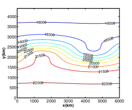
(a) Geopotential height field

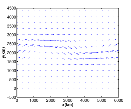
(b) Windfield

Figure 1: Initial condition: Geopotential height field for the Grammeltvedt initial condition and windfield (the velocity unit is 1km/s) calculated from the geopotential field using the geostrophic approximation.

Most of the depicted results are obtained in the case when the domain is discretized using a mesh of $376\times 276=103,776$ points, with $\Delta x=\Delta y=16$km. We select two integration time windows of $24$h and $3$h and we use $91$ time steps ($NT=91$) with $\Delta t=960$s and $\Delta t=120$s.

ADI FD SWE scheme proposed by Gustafsson 1971 in [37] is first employed in order to obtain the numerical solution of the SWE model. The implicit scheme allows us to integrate in time at a Courant-Friedrichs-Levy (CFL) condition of $\sqrt{gh}(\Delta t/\Delta x)<8.9301.$

The nonlinear algebraic systems of ADI FD SWE scheme is solved using quasi - Newton method, and the LU decomposition is performed every $6$ time steps.

We derive the reduced order models by employing a Galerkin projection.The POD basis functions are constructed using $91$ snapshots (number of snapshots equal with the number of time steps $N_{t}$) obtained from the numerical solution of the full - order ADI FD SWE model at equally spaced time steps for each time interval $[0,24h]$ and $[0,3h]$. Figures 2,3 show the decay around the eigenvalues of the snapshot solutions for $u,~{}v,~{}\phi$ and the nonlinear snapshots $F_{11},~{}F_{12},$ $F_{21},~{}F_{22}$, $F_{31},~{}F_{32}$. We notice that the singular values decay much faster when the model is integrated for $3$h. Consequently this translates in a more accurate solution representations for all three ROM methods using the same number of POD modes. For both time configurations and all tests in this study, the dimensions of the POD bases for each variable is taken to be $50$, capturing more than $99\%$ of the system energy. The largest neglected eigenvalues corresponding to state variables $u,~{}v,~{}\phi$ are $2.23,~{}1.16$ and $2.39$ for $t_{\rm f}=24$h and $0.0016,~{}0.0063$ and $0.0178$ for $t_{\rm f}=3$h, respectively.

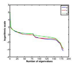
(a) State variables $u,~{}v,~{}\phi$

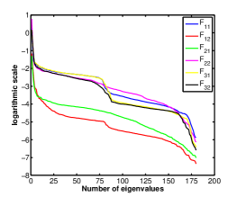
(b) Nonlinear terms

Figure 2: The decay around the singular values of the snapshots solutions for $u,~{}v,~{}\phi$ and nonlinear terms for $\Delta t=960s$ and integration time window of $24h$ .

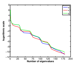
(a) State variables $u,~{}v,~{}\phi$

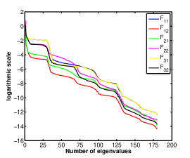
(b) Nonlinear terms

Figure 3: The decay around the singular values of the snapshots solutions for $u,~{}v,~{}\phi$ and nonlinear terms for $\Delta t=120s$ and a time integration window of $3h$ .

Next we apply DEIM algorithm and calculate the interpolation points to improve the efficiency of the standard POD approximation and to achieve a complexity reduction of the nonlinear terms with a complexity proportional to the number of reduced variables, as in the case of tensorial POD. Figures 4,5 illustrate the distribution of the first $100$ spatial points selected by the DEIM algorithm together with the isolines of the nonlinear terms statistics. Each of these statistics contain in every space location the maximum values of the corresponding nonlinear term over time. Maximum is preferred instead of time averaging since a better correlation between location of DEIM points and physical structures was observed in the former case.

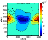
(a) Nonlinear term $F_{11}$

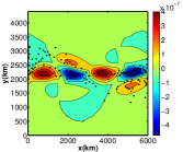
(b) Nonlinear term $F_{12}$

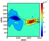
(c) Nonlinear term $F_{21}$

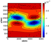
(d) Nonlinear term $F_{22}$

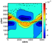
(e) Nonlinear term $F_{31}$

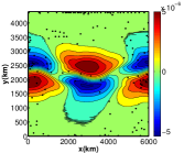
(f) Nonlinear term $F_{32}$

Figure 4: The first 100 DEIM interpolation points corresponding to all nonlinear terms in the SWE model for time integration window of $24h$. The background consists in isolines of the maximum values of the nonlinear terms over time.

However, in most cases, the spatial positions of the interpolation points don’t follow the nonlinear statistics structures. This is more visible in Figure 5 for $t_{\rm f}=3$h. The exceptions are $F_{12}$ and $F_{21}$ (Figures 5b,c), nonlinear terms depending only on velocity components, where DEIM interpolation points target better the underlying physical structures. This proves that DEIM algorithm doesn’t particularly take into account the physical structures of the nonlinear terms but search (in a greedy manner) to minimize the error (residual) between each column of the input basis (POD basis of the nonlinear term snapshots) and its proposed low-rank approximations Stefanescu and Navon [79, p.16].

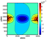
(a) Nonlinear term $F_{11}$

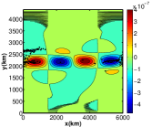
(b) Nonlinear term $F_{12}$

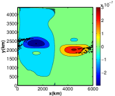
(c) Nonlinear term $F_{21}$

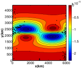
(d) Nonlinear term $F_{22}$

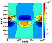
(e) Nonlinear term $F_{31}$

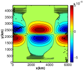
(f) Nonlinear term $F_{32}$

Figure 5: 100 DEIM interpolation points corresponding to all nonlinear terms in the SWE model for time integration window of $3h$. The background consists in isolines of the maximum values of the nonlinear terms over time. Most of the points are concentrated in the region with larger errors depicted in Figure 7.

Figures 6,7 depict the grid point absolute error of the standard POD, tensorial POD and POD/DEIM solutions with respect to the full solutions. For POD/DEIM reduced order model we use $180$ interpolation points. The magnitude of the errors are similar for each of the method proposed in this study. Moreover, we observed that error isolines distribution in Figure 7 is well correlated with the location of interpolation points illustrated in Figure 5 underlying the empirical characteristics of DEIM.

(a) $u_{\textnormal{\sc pod}}-u_{\textnormal{\sc full}}$

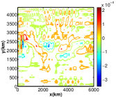
(b) $v_{\textnormal{\sc pod}}-v_{\textnormal{\sc full}}$

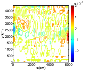
(c) $\phi_{\textnormal{\sc pod}}-\phi_{\textnormal{\sc full}}$

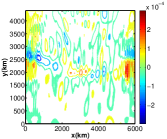
(d) $u_{\textnormal{\sc tpod}}-u_{\textnormal{\sc full}}$

(e) $v_{\textnormal{\sc tpod}}-v_{\textnormal{\sc full}}$

(f) $\phi_{\textnormal{\sc tpod}}-\phi_{\textnormal{\sc full}}$

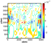
(g) $u_{\textnormal{\sc pod/deim}}-u_{\textnormal{\sc full}}$

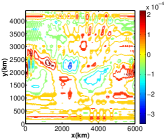
(h) $v_{\textnormal{\sc pod/deim}}-v_{\textnormal{\sc full}}$

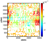
(i) $\phi_{\textnormal{\sc pod/deim}}-\phi_{\textnormal{\sc full}}$

Figure 6: Absolute errors between standard POD, tensorial POD and POD/DEIM solutions and the full trajectories at t = 24h ($\Delta t$ = 960s). The number of DEIM points was taken 180

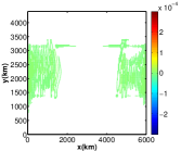
(a) $u_{\textnormal{\sc pod}}-u_{\textnormal{\sc full}}$

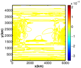
(b) $v_{\textnormal{\sc pod}}-v_{\textnormal{\sc full}}$

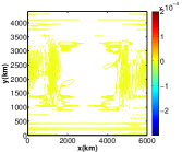
(c) $\phi_{\textnormal{\sc pod}}-\phi_{\textnormal{\sc full}}$

(d) $u_{\textnormal{\sc tpod}}-u_{\textnormal{\sc full}}$

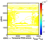
(e) $v_{\textnormal{\sc tpod}}-v_{\textnormal{\sc full}}$

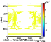
(f) $\phi_{\textnormal{\sc tpod}}-\phi_{\textnormal{\sc full}}$

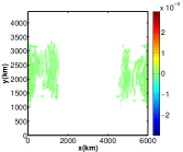
(g) $u_{\textnormal{\sc pod/deim}}-u_{\textnormal{\sc full}}$

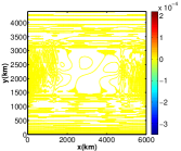
(h) $v_{\textnormal{\sc pod/deim}}-v_{\textnormal{\sc full}}$

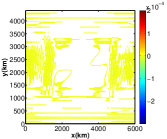
(i) $\phi_{\textnormal{\sc pod/deim}}-\phi_{\textnormal{\sc full}}$

Figure 7: Absolute errors between standard POD, tensorial POD and POD/DEIM solutions and the full trajectories at t = 3h ($\Delta t$ = 120s). The number of DEIM points was taken 180

In addition, we propose two metrics to quantify the accuracy level of standard POD, tensorial POD and standard POD/DEIM approaches. First, we use the following norm

$$\frac{1}{N_{t}}\sum_{i=1}^{t_{\rm f}}\frac{||w^{\textnormal{\sc full}}(:,t_{i})-w^{\textnormal{\sc rom}}(:,t_{i})||_{2}}{||w^{\textnormal{\sc full}}(:,t_{i})||_{2}}$$

$$\frac{1}{N_{t}}\sum_{i=1}^{N_{t}}\frac{\left\|w^{\textnormal{\sc full}}(:,t_{i})-w^{\textnormal{\sc rom}}(:,t_{i})\right\|_{2}}{\left\|w^{\textnormal{\sc full}}(:,t_{i})\right\|_{2}}$$

$i=1,2,..,t_{\rm f}$ and calculate the relative errors for all three variables of SWE model $w=(u,v,\phi)$. The results are presented in Table 3. We perform numerical experiments using two choices for number of DEIM points $70$ and $180$. For $24$h tests we notice that more than $70$ number of DEIM points are needed for convergence of quasi-Newton method for POD/DEIM SWE scheme explaining the absence of numerical results in Table 3 (left part).

Standard Tensorial POD/DEIM POD POD m=180 $u$ 1.276e-3 1.276e-3 1.622e-3 $v$ 3.426e-3 3.426e-3 4.639e-3 $\phi$ 2.110e-5 2.110e-5 2.489e-5 Standard Tensorial POD/DEIM POD/DEIM POD POD m = 180 m = 70 $u$ 7.711e-6 7.711e-6 7.965e-6 9.301e-6 $v$ 1.665e-5 1.666e-5 1.73e-5 1.975e-5 $\phi$ 1.389e-7 1.389e-7 1.426e-7 1.483e-7

Table 3: Relative errors for each of the model variables for $t_{f}=24$h (left) and $t_{f}=3$h (right). The POD bases dimensions were taken $50$. For $24$h experiments we display only the results for $180$ number of DEIM points while in the case of $3$h time integration window tests with $180$ and $70$ numbers of DEIM points are shown.

Root mean square error is also employed to compare the reduced order models. Table 4 and 5 show the RMSE for final times together with the CPU times of the on-line stage of ROMs.

Full ADI SWE Standard POD Tensorial POD POD/DEIM m=180 CPU time 1813.992s 191.785 2.491 1.046 $u$ - 9.095e-3 9.095e-3 1.555e-2 $v$ - 8.812e-3 8.812e-3 1.348e-2 $\phi$ - 6.987e-3e 6.987e-3 1.13e-2

Table 4: CPU time gains and the root mean square errors for each of the model variables at $t_{f}=24$h. Number of POD modes was $k=50$ and we choose $180$ number of DEIM points.

Full ADI SWE Standard POD Tensorial POD POD/DEIM m=180 POD/DEIM m=70 CPU time 950.0314s 161.907 2.125 0.642 0.359 $u$ - 5.358e-5 5.358e-5 5.646e-5 7.453e-5 $v$ - 2.728e-5 2.728e-5 3.418e-5 4.233e-5 $\phi$ - 8.505e-5e 8.505e-5 8.762e-5 9.212e-5

Table 5: CPU time gains and the root mean square errors for each of the model variables at $t_{f}=3$h for a $3$h time integration window. Number of POD modes was $k=50$ and two tests with different number of DEIM points $m=180,~{}70$ were simulated.

Thus, for $103,776$ spatial points, tensorial POD method reduces the computational complexity of the nonlinear terms in comparison with the POD ADI SWE model and overall decreases the computational time with a factor of $77\times$ for $24$h time integration and $76\times$ for a $3$h time window integration. POD/DEIM outperforms standard POD being $450\times$ and $250\times$ time faster for $70$ and $180$ DEIM interpolation points and a time integration window of $3h$. For $t_{\rm f}=24$h and $m=180$, POD/DEIM SWE model is $183\times$ time faster than standard POD SWE model. In terms of CPU time, tensor POD SWE model is only $2.38\times$ slower than POD/DEIM SWE model for $m=180$ and $t_{\rm f}=24$h while for $t_{\rm f}=3$h the new tensorial POD scheme is $5.9\times$ and $3.3\times$ less efficient than POD/DEIM SWE model for $m=70$ and $m=180$. This suggests that operations like Jacobian computations and its LU decomposition required by both reduced order approaches weight more in the overall CPU time cost since the quadratic nonlinear complexity of the tensorial POD requires $374,950$ floating-point operations and POD/DEIM only $27,180$ ($m=180$, see Section $3$). Given that the implementation effort is much reduced, in the cases of models depending only on quadratic nonlinearities, the tensorial POD poses the appropriate characteristics of a reduced order method and represent a solid alternative to the POD/DEIM approach.

For cubical nonlinearities and larger, tensorial POD loses its ability to deliver fast calculations (see Table 1), thus the POD/DEIM should be employed.

In our case the Jacobians are calculated analytically and its computations depend only on the reduced space dimension $k$. However, more gain can be obtain if DEIM would be applied to approximate the reduced Jacobians but this is subject of future research.

The computational savings and accuracy levels obtained by the ROMs studied in this paper depend on the number of POD modes and number of DEIM points. These numbers may be large in practice in order to capture well the full model dynamics. For exemple, in the case of a time window integration of $24$h, if someone would ask to increase the ROMs solutions accuracy with only one order of magnitude, the POD basis dimension must be at least larger than $100$ which will drastically compromise the time performances of ROMs methods. Elegant solutions to this problem were proposed by Rapún and Vega [65], Peherstorfer et al. [64] where local POD and local DEIM versions were proposed. Machine learning techniques such as $K$-means Lloyd [52], MacQueen [55], Steinhaus [80] can be used for both time and space partitioning. A recent study investigating cluster-based reduced order modeling was proposed by Kaiser et al. [44].

Figure 8 depicts the efficiency of tensorial POD and POD/DEIM SWE schemes as a function of spatial discretization points in the case of $t_{\rm f}=3$h. We compare the results obtained for $8$ different mesh configurations $n=31\times 23,~{}61\times 45,~{}101\times 71,~{}121\times 89,~{}151\times 111,~{}241\times 177,~{}301\times 221,~{}376\times 276$. CPU time performances of the off-line and on-line stages of the ROMs SWE schemes are compared since reduced order optimization algorithms include both phases.

For the on-line stage, once the number of spatial discretization points is larger than $151\times 111$ tensorial POD scheme is $10\times$ faster than the standard POD scheme. The performances of POD/DEIM depends on the number of DEIM points and the numerical results displays a $10\times$ time reduction of the CPU costs in comparison with the standard POD outcome when $n\geq 61\times 45$ and $n\geq 101\times 71$ for $m=70$ and $m=180$ respectively.

The new algorithm introduced in Section $3$ relying on DEIM interpolation points delivers fast tensorial calculations required for computing the reduced Jacobian in the on-line stage and thus allowing POD/DEIM SWE scheme to have the fastest off-line stage (Figure 9b). This gives a good advantage of ROM optimization based on Discrete Empirical Interpolation Method supposing that quality approximations of nonlinear terms and reduced Jacobians are delivered since during optimization input data are different than the ones used to generate the DEIM interpolation points. DEIM was first employed by Baumann [9] to solve a reduced 4D-Var data assimilation problem and good results were obtained for a 1D Burgers model. Extensions to 2D models are still not available in the literature.

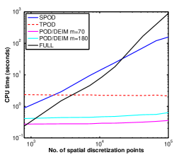
(a) On-line stage

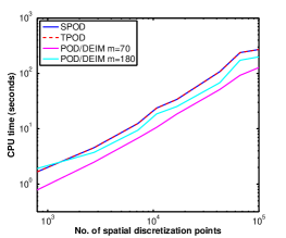
(b) Off-line stage

Figure 8: Cpu time vs. the number of spatial discretization points for $t_{\rm f}=3$h ; number of POD modes = 50; two different numbers of DEIM points $70$ and $180$ have been employed.

7 Conclusions

It is well known that in standard POD the cost of evaluating nonlinear terms during the on-line stage depends on the full space dimension, and this constitutes a major efficiency bottleneck. The present manuscript applies tensorial calculus techniques which allows fast computations of standard POD reduced quadratic nonlinearities. We show that tensorial POD can be applied to all type of polynomial nonlinearities and the resulting nonlinear terms have a complexity of $\mathcal{O}(k^{p+1})$ operations, where $k$ is the dimension of POD subspace and $p$ is the polynomial degree. Consequently, this approach eliminates the dependency on the full space dimension, while yielding the same reduced solution accuracy as standard POD. Despite being independent of number of mesh points, tensorial POD is efficient only for quadratic nonlinear terms since for higher nonlinearities standard POD proves to be less time consuming once the POD basis dimension $k$ is increased.

The efficiency of tensorial POD is compared against that of standard POD and of POD/DEIM. We theoretically analyze the number of floating-point operations required as a function of polynomial degree $p$, the number of degrees of freedom of the high-fidelity model $n$, of POD modes $k$, and of DEIM interpolation points $m$. For quadratic nonlinearities and $k$ between $10$–$50$ modes, the tensorial POD needs $10$–$40$ times fewer operations than the standard POD approach and $10$–$20$ times more operations than the POD/DEIM with $m=100$. But these performances are not translated into the same CPU time rates for solving the ROMs solutions since other more time consuming calculations are needed.

Numerical experiments are carried out using a two dimensional ADI SWE finite difference model. Reduced order models were developed using each of the three ROM methods and Galerkin projection. The spectral analysis of snapshots matrices reveals that local versions of ROMs lead to more accurate results. Consequently, we focus on three hours time integration windows. The tensorial POD SWE model becomes considerably faster than standard POD when the dimension of the full model increases. For example, for $100,000$ spatial points the tensorial POD SWE model yields the same solutions accuracy as standard POD but is $76$ times faster. Numerical experiments of POD/DEIM SWE scheme revealed a considerable reduction of the computational complexity. For a number of $70$ DEIM points, POD/DEIM SWE model is $450$ times faster than standard POD, but only $6$ times faster than tensorial POD.

For models depending only on quadratic nonlinearities, the tensorial POD represents a solid alternative to POD/DEIM where the implementation effort is considerably larger. However, for cubic and higher order nonlinearities, tensorial POD loses its ability to deliver fast calculations and the POD/DEIM approach should be employed.

We also propose a new DEIM-based algorithm that allows fast computations of the tensors needed by reduced Jacobians calculations in the on-line stage. The resulting off-line POD/DEIM stage is the fastest among the ones considered here, even if additional SVD decompositions and low-rank terms are computed. This is an important advantage in optimization problems based on POD/DEIM surrogates where the reduced order bases need to be updated multiple times.

On-going work by the authors focuses on reduced order constrained optimization. The current research represents an important step toward developing tensorial POD and POD/DEIM four dimensional variational data assimilation systems, which are not available in the literature for complex models.

References

- Aanonsen [2009] T. O. Aanonsen. Empirical interpolation with application to reduced basis approximations. PhD thesis, Norwegian University of Science and Technology, 2009.
- Amsallem et al. [2011] D. Amsallem, J. Cortial, K. Carlberg, and C. Farhat. A method for interpolating on manifolds structural dynamics reduced-order models. International Journal for Numerical Methods in Engineering, 80(9):1241–1257, 2011.
- Antoulas [2005] A.C. Antoulas. Approximation of Large-Scale Dynamical Systems. Advances in Design and Control. SIAM, Philadelphia, 2005.
- Antoulas [2009] A.C. Antoulas. Approximation of large-scale dynamical systems. Society for Industrial and Applied Mathematics, 6:376–377, 2009.
- Astrid et al. [2008] P. Astrid, S. Weiland, K. Willcox, and T. Backx. Missing point estimation in models described by Proper Orthogonal Decomposition. IEEE Transactions on Automatic Control, 53(10):2237–2251, 2008.
- Baker et al. [1996] M. Baker, D. Mingori, and P. Goggins. Approximate Subspace Iteration for Constructing Internally Balanced Reduced-Order Models of Unsteady Aerodynamic Systems. AIAA Meeting Papers on Disc, pages 1070–1085, 1996.
- Barrault et al. [2004] M. Barrault, Y. Maday, N.C. Nguyen, and A.T. Patera. An ’empirical interpolation’ method: application to efficient reduced-basis discretization of partial differential equations. Comptes Rendus Mathematique, 339(9):667–672, 2004.
- Barrett et al. [1994] R. Barrett, M. Berry, T. F. Chan, J. Demmel, J. Donato, J. Dongarra, V. Eijkhout, R. Pozo, C. Romine, and H. Van der Vorst. Templates for the Solution of Linear Systems: Building Blocks for Iterative Methods, 2nd Edition. SIAM, Philadelphia, PA, 1994.
- Baumann [2013] M.M. Baumann. Nonlinear Model Order Reduction using POD/DEIM for Optimal Control of Burgersâquation. Master’s thesis, Delft University of Technology, Netherlands, 2013.
- Belzen and Weiland [2012] F. Belzen and S. Weiland. A tensor decomposition approach to data compression and approximation of ND systems. Multidimensional Systems and Signal Processing, 23(1-2):209–236, 2012.
- Benner and Breiten [2012] P. Benner and T. Breiten. Two-sided moment matching methods for nonlinear model reduction. Technical Report MPIMD/12-12, Max Planck Institute Magdeburg Preprint, June 2012.
- Benner and Sokolov [2006] P. Benner and V.I. Sokolov. Partial realization of descriptor systems. Systems Control Letters, 55(11):929 –938, 2006.
- Benner et al. [2013] P. Benner, S. Gugercin, and K. Willcox. A survey of model reduction methods for parametric systems. Technical Report MPIMD/13-14, Max Planck Institute Magdeburg Preprint, August 2013.
- Bo [2011] Nguyen Van Bo. Computational simulation of detonation waves and model reduction for reacting flows. PhD thesis, Singapore-MIT alliance, National University of Singapore, 2011.
- Bui-Thanh et al. [2004] T. Bui-Thanh, M. Damodaran, and K. Willcox. Aerodynamic data reconstruction and inverse design using proper orthogonal decomposition. AIAA Journal, pages 1505–1516, 2004.
- Bultheel and Moor [2000] A. Bultheel and B. De Moor. Rational approximation in linear systems and control. Journal of Computational and Applied Mathematics, 121:355–378, 2000.
- Carlberg and Farhat [2011] K. Carlberg and C. Farhat. A low-cost, goal-oriented compact proper orthogonal decomposition basis for model reduction of static systems. International Journal for Numerical Methods in Engineering, 86(3):381–402, 2011.
- Carlberg et al. [2011] K. Carlberg, C. Bou-Mosleh, and C. Farhat. Efficient non-linear model reduction via a least-squares Petrov- Galerkin projection and compressive tensor approximations. International Journal for Numerical Methods in Engineering, 86(2):155–181, 2011.
- Carlberg et al. [2012] K. Carlberg, R. Tuminaro, and P. Boggsz. Efficient structure-preserving model reduction for nonlinear mechanical systems with application to structural dynamics. preprint, Sandia National Laboratories, Livermore, CA 94551, USA, 2012.
- Chaturantabut [2008] S. Chaturantabut. Dimension Reduction for Unsteady Nonlinear Partial Differential Equations via Empirical Interpolation Methods. Technical Report TR09-38,CAAM, Rice University, 2008.
- Chaturantabut and Sorensen [2011] S. Chaturantabut and D .C. Sorensen. Application of POD and DEIM on dimension reduction of non-linear miscible viscous fingering in porous media. Mathematical and Computer Modelling of Dynamical Systems, 17(4):337–353, 2011.
- Chaturantabut and Sorensen [2010] S. Chaturantabut and D.C. Sorensen. Nonlinear model reduction via discrete empirical interpolation. SIAM Journal on Scientific Computing, 32(5):2737–2764, 2010.
- Chaturantabut and Sorensen [2012] S. Chaturantabut and D.C. Sorensen. A state space error estimate for POD-DEIM nonlinear model reduction. SIAM Journal on Numerical Analysis, 50(1):46–63, 2012.
- Dihlmann and Haasdonk [2013] M. Dihlmann and B. Haasdonk. Certified PDE-constrained parameter optimization using reduced basis surrogate models for evolution problems. Submitted to the Journal of Computational Optimization and Applications, 2013. URL http://www.agh.ians.uni-stuttgart.de/publications/2013/DH13.
- Everson and Sirovich [1995] R. Everson and L. Sirovich. Karhunen -Loeve procedure for gappy data. Journal of the Optical Society of America A, 12:1657–64, 1995.
- Fairweather and Navon [1980] G. Fairweather and I.M. Navon. A linear ADI method for the shallow water equations. Journal of Computational Physics, 37:1–18, 1980.
- Feldmann and Freund [1995] P. Feldmann and R.W. Freund. Efficient linear circuit analysis by Pade approximation via the Lanczos process. IEEE Transactions on Computer-Aided Design of Integrated Circuits and Systems, 14:639–649, 1995.
- Freund [2003] R.W. Freund. Model reduction methods based on Krylov subspaces. Acta Numerica, 12:267–319, 2003.
- Gallivan et al. [1994] K. Gallivan, E. Grimme, and P. Van Dooren. Padé approximation of large-scale dynamic systems with lanczos methods. In Decision and Control, 1994., Proceedings of the 33rd IEEE Conference on, volume 1, pages 443–448 vol.1, Dec 1994.
- Gragg [1972] W.B. Gragg. The Padé table and its relation to certain algorithms of numerical analysis. SIAM Review, 14:1–62, 1972.
- Gragg and Lindquist [1983] W.B. Gragg and A. Lindquist. On the partial realization problem. Linear Algebra and Its Applications, Special Issue on Linear Systems and Control, 50:277 –319, 1983.
- Grammeltvedt [1969] A. Grammeltvedt. A survey of finite difference schemes for the primitive equations for a barotropic fluid. Monthly Weather Review, 97(5):384–404, 1969.
- Grepl and Patera [2005] M.A. Grepl and A.T. Patera. A posteriori error bounds for reduced-basis approximations of parametrized parabolic partial differential equations. ESAIM: Mathematical Modelling and Numerical Analysis, 39(01):157–181, 2005.
- Grepl et al. [2007] M.A. Grepl, Y. Maday, N.C. Nguyen, and A.T. Patera. Efficient reduced-basis treatment nofonaffine and nonlinear partial differential equations. Modélisation Mathématique et Analyse Numérique, 41(3):575–605, 2007.
- Grimme [1997] E.J. Grimme. Krylov projection methods for model reduction. PhD thesis, Univ. Illinois, Urbana-Champaign, 1997.
- Gudmundsson and Laub [1994] T. Gudmundsson and A. Laub. Approximate Solution of Large Sparse Lyapunov Equations. IEEE Transactions on Automatic Control, 39(5):1110–1114, 1994.
- Gustafsson [1971] B. Gustafsson. An alternating direction implicit method for solving the shallow water equations. Journal of Computational Physics, 7:239–254, 1971.
- Gutknecht [1994] M.H. Gutknecht. The Lanczos process and Padé approximation. Proc. Cornelius Lanczos Intl. Centenary Conference, edited by J.D. Brown et al., SIAM, Philadelphia, pages 61–75, 1994.
- Hinze and Kunkel [2012] M. Hinze and M. Kunkel. Discrete Empirical Interpolation in POD Model Order Reduction of Drift-Diffusion Equations in Electrical Networks. Scientific Computing in Electrical Engineering SCEE 2010 Mathematics in Industry, 16(5):423–431, 2012.
- Hochman et al. [2011] A. Hochman, B.N. Bond, and J.K. White. A stabilized discrete empirical interpolation method for model reduction of electrical thermal and microelectromechanical systems. Design Automation Conference (DAC), 48th ACM/EDAC/IEEE, pages 540–545., 2011.
- Hodel [1991] A.S. Hodel. Least Squares Approximate Solution of the Lyapunov Equation. Proceedings of the 30th IEEE Conference on Decision and Control, IEEE Publications, Piscataway, NJ, 1991.
- Hotelling [1933] H. Hotelling. Analysis of a complex of statistical variables with principal components. Journal of Educational Psychology, 24:417–441, 1933.
- Jaimoukha and Kasenally [1994] I. Jaimoukha and E. Kasenally. Krylov Subspace Methods for Solving Large Lyapunov Equations. SIAM Journal of Numerical Analysis, 31(1):227–251, 1994.
- Kaiser et al. [2013] E. Kaiser, Bernd R. Noack, L. Cordier, A. Spohn, M. Segond, M. Abel, G. Daviller, and R.K. Niven. Cluster-based reduced-order modelling of a mixing layer. Technical Report arXiv:1309.0524 [physics.flu-dyn], Cornell University, September 2013.
- Karhunen [1946] K. Karhunen. Zur spektraltheorie stochastischer prozesse. Annales Academiae Scientarum Fennicae, 37, 1946.
- Kellems et al. [2010] A. R. Kellems, S. Chaturantabut, D. C. Sorensen, and S. J. Cox. Morphologically accurate reduced order modeling of spiking neurons. Journal of Computational Neuroscience, 28:477–494, 2010.
- Kelley [1995] C. T. Kelley. Iterative Methods for Linear and Nonlinear Equations. Number 16 in Frontiers in Applied Mathematics. SIAM, 1995.
- Kunisch and Volkwein [1999] K. Kunisch and S. Volkwein. Control of the Burgers Equation by a Reduced-Order Approach Using Proper Orthogonal Decomposition. Journal of Optimization Theory and Applications, 102(2):345–371, 1999.
- Kunisch and Volkwein [2002] K. Kunisch and S. Volkwein. Galerkin Proper Orthogonal Decomposition Methods for a General Equation in Fluid Dynamics. SIAM Journal on Numerical Analysis, 40(2):492–515, 2002.
- Kunisch et al. [2004] K. Kunisch, S. Volkwein, and L. Xie. HJB-POD-Based Feedback Design for the Optimal Control of Evolution Problems. SIAM J. Appl. Dyn. Syst, 3(4):701–722, 2004.
- Lass and Volkwein [2012] O. Lass and S. Volkwein. POD Galerkin schemes for nonlinear elliptic-parabolic systems. Konstanzer Schriften in Mathematik, 301:1430–3558, 2012.
- Lloyd [1957] S. Lloyd. Least squares quantization in PCM. IEEE Trans. Inform. Theory, 28:129–137, 1957.
- Loève [1955] M.M. Loève. Probability Theory. Van Nostrand, Princeton, NJ, 1955.
- Lorenz [1956] E.N. Lorenz. Empirical Orthogonal Functions and Statistical Weather Prediction. Technical report, Massachusetts Institute of Technology, Dept. of Meteorology, 1956.
- MacQueen [1967] J. MacQueen. Some methods for classification and analysis of multivariate observations. Proceedings of the Fifth Berkeley Symposium on Mathematical Statistics and Probability, 1:281–297, 1967.
- Maday et al. [2009] Y. Maday, N.C. Nguyen, A.T. Patera, and G.S.H. Pau. A General Multipurpose Interpolation Procedure: the Magic Points. Communications on Pure and Applied Analysis, 8(1):383–404, 2009.
- Moore [1981] B.C. Moore. Principal component analysis in linear systems: Controllability, observability, and model reduction. IEEE Transactions on Automatic Control, 26(1):17–32, 1981.
- Mullis and Roberts [1976] C.T. Mullis and R.A. Roberts. Synthesis of Minimum Roundoff Noise Fixed Point Digital Filters. IEEE Transactions on Circuits and Systems, CAS-23:551–562, 1976.
- Navon and Villiers [1986] I. M. Navon and R. De Villiers. Gustaf: A Quasi-Newton nonlinear ADI fortran iv program for solving the shallow-water equations with augmented lagrangians. Computers and Geosciences, 12(2):151–173, 1986.
- Nguyen et al. [2008] N.C. Nguyen, A.T. Patera, and J. Peraire. A ’best points’ interpolation method for efficient approximation of parametrized function. International Journal for Numerical Methods in Engineering, 73:521–543, 2008.
- Noack et al. [2003] B.R. Noack, K. Afanasiev, M. Morzynski, G. Tadmor, and F. Thiele. A hierarchy of low-dimensional models for the transient and post-transient cylinder wake. Journal of Fluid Mechanics, 497:335–363, 2003. ISSN 0022-1120.
- Noack et al. [2010] B.R. Noack, M. Schlegel, M. Morzynski, and G. Tadmor. System reduction strategy for galerkin models of fluid flows. International Journal for Numerical Methods in Fluids, 63(2):231–248, 2010.
- Patera and Rozza [2007] A.T. Patera and G. Rozza. Reduced basis approximation and a posteriori error estimation for parametrized partial differential equations, 2007.
- Peherstorfer et al. [2013] B. Peherstorfer, D. Butnaru, K. Willcox, and H.J. Bungartz. Localized Discrete Empirical Interpolation Method. MIT Aerospace Computational Design Laboratory Technical Report TR-13-1, 2013.
- Rapún and Vega [2010] M.L. Rapún and J.M. Vega. Reduced order models based on local POD plus Galerkin projection. Journal of Computational Physics, 229(8):3046–3063, 2010.
- Rewieński and White [2001] M. Rewieński and J. White. A Trajectory Piecewise-linear Approach to Model Order Reduction and Fast Simulation of Nonlinear Circuits and Micromachined Devices. In Proceedings of the 2001 IEEE/ACM International Conference on Computer-aided Design, ICCAD ’01, pages 252–257, Piscataway, NJ, USA, 2001. IEEE Press.
- Rowley et al. [2004] C. W. Rowley, T. Colonius, and R. M. Murray. Model reduction for compressible flows using POD and Galerkin projection. Physica D. Nonlinear Phenomena, 189(1–2):115–129, 2004.
- Rowley [2005] C.W. Rowley. Model Reduction for Fluids, using Balanced Proper Orthogonal Decomposition. International Journal of Bifurcation and Chaos (IJBC), 15(3):997–1013, 2005.
- Rowley et al. [2009] C.W. Rowley, I. Mezic, S. Bagheri, P.Schlatter, and D.S. Henningson. Spectral analysis of nonlinear flows. Journal of Fluid Mechanics, 641:115–127, 2009.
- Rozza et al. [2008] G. Rozza, D.B.P. Huynh, and A.T. Patera. Reduced basis approximation and a posteriori error estimation for affinely parametrized elliptic coercive partial differential equations. Archives of Computational Methods in Engineering, 15(3):229–275, 2008.
- Saad [1994] Y. Saad. Sparsekit: a basic tool kit for sparse matrix computations. Technical Report, Computer Science Department, University of Minnesota, 1994.
- Saad [2003] Y. Saad. Iterative Methods for Sparse Linear Systems. Society for Industrial and Applied Mathematics, Philadelphia, PA, USA, 2nd edition, 2003.
- San and Iliescu [2013] O. San and T. Iliescu. Proper orthogonal decomposition closure models for fluid flows: Burgers equation. Technical Report arXiv:1308.3276 [physics.flu-dyn], Cornell University, August 2013.
- Schmid [2010] P.J. Schmid. Dynamic mode decomposition of numerical and experimental data. Journal of Fluid Mechanics, 656:5–28, 2010.
- Sirovich [1987a] L. Sirovich. Turbulence and the dynamics of coherent structures. I. Coherent structures. Quarterly of Applied Mathematics, 45(3):561–571, 1987a. ISSN 0033-569X.
- Sirovich [1987b] L. Sirovich. Turbulence and the dynamics of coherent structures. II. Symmetries and transformations. Quarterly of Applied Mathematics, 45(3):573–582, 1987b. ISSN 0033-569X.
- Sirovich [1987c] L. Sirovich. Turbulence and the dynamics of coherent structures. III. Dynamics and scaling. Quarterly of Applied Mathematics, 45(3):583–590, 1987c. ISSN 0033-569X.
- Sorensen and Antoulas [2002] D.C. Sorensen and A.C. Antoulas. The Sylvester equation and approximate balanced reduction. Linear Algebra and its Applications, 351-352(0):671–700, 2002.
- Stefanescu and Navon [2013] R. Stefanescu and I.M. Navon. POD/DEIM Nonlinear model order reduction of an ADI implicit shallow water equations model. Journal of Computational Physics, 237:95–114, 2013.
- Steinhaus [1956] H. Steinhaus. Sur la division des corps matériels en parties. Bulletin of the Polish Academy of Sciences, 4(12):801–804, 1956.
- Suwartadi [2012] E. Suwartadi. Gradient-based Methods for Production Optimization of Oil Reservoirs. PhD thesis, Mathematics and Electrical Engineering, Department of Engineering Cybernetics,Norwegian University of Science and Technology, 2012.
- Tissot et al. [2013] G. Tissot, L. Cordier, N. Benard, and B.R. Noack. Dynamic mode decomposition of PIV measurements for cylinder wake flow in turbulent regime. In Proceedings of the 8th International Symposium On Turbulent and Shear Flow Phenomena, TSFP-8, 2013.
- Tonn [2012] T. Tonn. Reduced-Basis Method (RBM) for Non-Affine Elliptic Parametrized PDEs. (PhD), Ulm University, 2012.
- Van Dooren [1995] P. Van Dooren. The Lanczos algorithm and Padé approximations. In Short Course, Benelux Meeting on Systems and Control, 1995.
- Willcox and Peraire [2002] K. Willcox and J. Peraire. Balanced model reduction via the Proper Orthogonal Decomposition. AIAA Journal, pages 2323–2330, 2002.
- Wirtz et al. [2012] D. Wirtz, D.C. Sorensen, and B. Haasdonk. A-posteriori error estimation for DEIM reduced nonlinear dynamical systems. SRC SimTech Preprint Series, 2012.
- Xiao et al. [2014] D. Xiao, F. Fang, A.G. Buchan, C.C. Pain, I.M. Navon, J. Du, and G. Hu. Non-linear model reduction for the Navier-Stokes equations using residual DEIM method. Journal of Computational Physics, 263:1–18, 2014. ISSN 0021-9991.
- Zhou [2012] Y.B. Zhou. Model reduction for nonlinear dynamical systems with parametric uncertainties. (M.S), Massachusetts Institute of Technology, Dept. of Aeronautics and Astronautics, 2012.