Coalitions of pulse-interacting dynamical units

Abstract

We prove that large global systems of interacting (non necessarily similar) dynamical units that are coupled by cooperative impulses, recurrently exhibit the so called grand coalition , for which all the units arrive to their respective goals simultaneously. We bound from above the waiting time until the first grand coalition appears. Finally, we prove that if besides the units are mutually similar, then the grand coalition is the unique subset of goal-synchronized units that is recurrently shown by the global dynamics.

MSC 2010:   Primary: 37NXX, 92B20; Secondary: 34D06, 05C82, 94A17, 92B25
Keywords: Pulse-coupled networks, interacting dynamical units, coalitions, synchronization

1 Introduction

We study the global dynamics of a network $N$ composed by a large number $m$ of dynamical units that mutually interact by cooperative (i.e. positive) instantaneous pulses.

One of the most cited examples of the type of phenomena that we are contributing to explain mathematically along this work, is the large scale synchronization of the flashes of the fireflies “Pteroptyx malaccae”: a large number of individuals flash periodically all together after a waiting time, when they meet together on trees, with neither an external clock nor privileged individuals mastering the global synchronization [10].

We are motivated on the study of the dynamics of such global systems to obtain abstract and very general mathematical results, that are independent of the concrete formulae governing the dynamics, and require very few hypothesis. They are applicable in particular to models used in Neuroscience for which more or less concrete formulae and hypothesis governing the individual dynamics of the neurons are assumed (see for instance [2, 11, 13, 17, 23]).

The mathematical study of the global dynamics of abstract and general networks composed by mutually interacting units has a large diversity of concrete applications to other sciences and technology. As said above, they are widely used in Neuroscience. They have also applications to Engineering, for instance in the design and construction of some systems used in communications [27, 28]; also to Physics, for instance in the study of systems of light controlled oscillators [21, 22], and in the research of the evolution of physical lattices of coupled dynamical units of different nature [8, 26]. They have other important applications to Biology, for instance in the research of mathematical models of genetic regulatory networks [9]; to Ecology, in the study of the equilibria of some ecological systems evolving on time [12, 25]; to Economy and other social sciences, in the research of coupled networks of different agents, individuals or coalitions of individuals, for instance by means of evolutive Game Theory [18, 1].

While not interacting with the other units of the network, each unit $i\in\{1,2,\ldots,m\}$, which we also call “cell”, evolves governed by two rules that determine the “free dynamics of $i$”: the relaxation rule and the update rule, which we will precisely define in Subsection 2.1. While the units are not interacting, the dynamics of the network is the product dynamics of its $m$ units, which evolve independently one from the other. But at certain instants, at least one unit $i$ changes the dynamical rules that govern the other units $j\neq i$. The instants when each unit $i$ acts on the others are exclusively determined by the state $x_{i}$ of $i$. The pulsed coupling hypothesis assumes that any action from $i$ to $j\neq i$ is a discontinuity jump in the instantaneous state of the cell $j$ according to the interactions rules which we will precisely define in Subsection 2.1.

The free dynamics rules and the instantaneous interactions rules, as well as the mathematical results that we obtain from them, generalize to a wide context the particular cases that were studied for instance in [19, 3, 7, 14, 6].

The results that we prove along the paper deal with the spontaneous formation of coalitions (subsets) of dynamical units during the dynamical evolution of the network, provided that the interactions among the units are all “cooperative” (i.e. positively signed). Roughly speaking, each coalition is a subset of units that synchronize certain milestones of their respective individual dynamics, which we call goals, and do that spontaneously without any external clock or master unit, infinitely many times in the future. In particular the formation of the so called grand coalition (i.e. the simultaneous arrival to a certain goal of all the units of the network) is spontaneously and recurrently exhibited from any initial state (Theorem 2.8). The synchronization in the grand coalition was initially proved in 1992 by Mirollo and Strogatz [19], under restrictive hypothesis requiring that the units were identical, the interactions were also identical, and that the free dynamics of the units were one-dimensional oscillators whose evolution were linear on time. Later, in 1996, Bottani [3] proved the synchronization of the grand coalition requiring that the units were similar (non necessarily identical), but still one dimensional oscillators although their evolution were not necessarily linear on time. In Theorem 2.8 we will generalize the result to any network of non necessarily similar units with cooperative interactions that depend on the pair of interacting cells, with general free dynamics of each unit $i$, on any finite dimension (depending on $i$), and such that the cells do not necessarily behave as oscillators. The price to pay for such a general result is that the network has to be large enough, and, unless the units were mutually similar (Theorem 2.10), the grand coalition is not necessarily the unique coalition that is exhibited recurrently in the future.

Due to the fact that the units may be very different and that the grand coalition is not necessarily the unique coalition that is exhibited in the future, the word “synchronization” in Theorem 2.8, if applied, it is not in its classical meaning ([20]). In fact, the orbits of each of the units that recurrently exhibit the grand coalition, are not synchronized in the strict sense since they do not show the same state for all the instants $t\geq 0$. The states of two or more units may sensibly differ one from the others, at some instants between two consecutive formations of the grand coalition.

On the one hand, the synchronization in the strict or wide sense, for models of pulsed coupled dynamical units, were up to now proved for particular examples in which the free dynamics of each cell is governed by a differential equation or a discrete time mapping with a concrete formulae. For instance, the free dynamics is governed by affine mapping in [7], by linear differential equations in [21, 22], and by piecewise contracting maps in [26] [14],[6] or using known results about piecewise contractions in [4]. In this sense, the novelty of the results here is that their proofs work independently of the concrete formulation of the free dynamics of the cells. They have almost no hypothesis about the second term of the differential equation governing the free dynamics of each of the cells.

On the other hand, the results along this paper hold independently of the dimension of the space $X_{i}$ where the state of each unit evolves, and they do not require the free dynamics of each unit to make it an oscillator. This freedom allows the results to be applied for instance to multidimensional chaotic free dynamics of the cells that recurrently shear certain milestones in the global collective dynamics ([15, 16]).

The paper is organized as follows: in Section 2 we state the mathematical definitions and theorems to be proved. In Section 3 we write the proofs.

2 Definitions and statements of the results

2.1 Definitions and hypothesis

The relaxation rule of the free dynamics of $i$:

The relaxation rule of the free dynamics of the cell $i$ determines the evolution on time $t\geq 0$ of the state $x_{i}$ on a compact finite-dimensional manifold $X_{i}$ (whose dimension may depend of $i$). It is defined as the solution of any differential equation:

$$\frac{dx_{i}}{dt}=f_{i}(x_{i}),\ \ \ x_{i}\in X_{i}$$ (1)

satisfying just one condition as follows:

There exists a Lyapunov real function $S_{i}:X_{i}\mapsto\mathbb{R}$, which we call the satisfaction level of $i$, such that:

$$\frac{dS_{i}(x_{i}(t))}{dt}=\bigtriangledown S_{i}(x_{i}(t))\cdot f_{i}(x_{i}(t))>v_{i}>0\ \ \forall\ t\mbox{ such that }S_{i}(x_{i}(t))<\theta_{i},$$ (2)

where $\theta_{i}$ is a positive constant (for each unit $i$) which we call the goal of $i$. (In formula (2) $\bigtriangledown S_{i}\cdot f_{i}$ denotes the inner product in the tangent bundle of the manifold $X_{i}$).

In other words, the free dynamics of $i$ holds at all the instants for which $i$ is uncoupled to the network and its state is unchanged by interferences that may come from outside $i$. It is described by a finite dimensional variable $x_{i}$ evolving on time $t$ in such a way that the satisfaction level $S_{i}(x_{i})$, while it does not reach the goal value $\theta_{i}$, is strictly increasing with $t$ and its (positive) velocity is bounded away from zero.

The update rule of the free dynamics of $i$:

The update rule is a discontinuity jump in the state $x_{i}$ of the cell $i$ that is produced whenever the satisfaction variable $S_{i}(x_{i}(t))$ reaches (or is larger than) the goal level $\theta_{i}$. This discontinuity jump instantaneously resets the satisfaction level $S_{i}(x_{i}(t))$ to a “reset value”, which is strictly smaller than $\theta_{i}$. With no loss of generality, we assume that the reset value is zero (see Figure 1). Precisely:

$$S_{i}(x_{i}(t_{0}^{-}))\geq\theta_{i}\ \ \Rightarrow\ \ S_{i}(x_{i}(t_{0}))=0,$$ (3)

where $S_{i}(x_{i}(t_{0}^{-}))$ denotes $\lim_{t\rightarrow t_{0}^{-}}S_{i}(x_{i}(t))$.

Note that the alternation between the relaxation and update rules of the free dynamics of $i$ will occur while no interferences come from outside $i$ forcing its satisfaction variable to decrease (see Figure 1). Nevertheless, the free evolution $S_{i}(x_{i}(t))$ is not necessarily periodic if $\mbox{dim}(X_{i})\geq 2$. In fact, the set $S_{i}^{-1}(\{0\})\subset X_{i}$ of states with constant null satisfaction may be for instance a curve: there may exist infinitely many points in $X_{i}$ for which $S_{i}=0$. So, each state $x_{i}(t)$ obtained from the reset rule $S_{i}(x_{i}(t))=0$ from the goal $S_{i}(x_{i}(t^{-}))=\theta_{i}$, does not necessarily repeat in the future to make the evolution $S_{i}(x_{i}(t))$ periodic with an exact time-period. On the contrary, if the set of all the possible reset states $x_{i}\in S_{i}^{-1}(\{0\})$ were finite (this can occur even if $S_{i}^{-1}(\{0\})$ is infinite), then the free dynamics of $i$ would make it be periodic, i.e. an oscillator.

Definition 2.1

(Spikes) Taking the name from Neuroscience, we call spike of the cell $i$ to the discontinuity jump of its satisfaction state from the goal value $\theta_{i}$ (which in Neuroscience is called “threshold level”) to its reset value (which is assumed to be zero). Note that the instants when each cell $i$ spikes, while not interacting with the other units of the network, are defined just by the value of its own satisfaction variable. There is neither an external clock nor a master unit in the network to force a synchronization of the spikes of the many cells of the network.

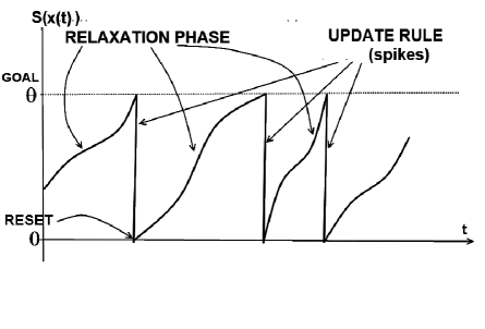
Figure 1: The evolution on time $t$ of the satisfaction variable $S(x(t))$ of a dynamical unit while not interacting with the other units of the network.

The interactions rules among the units

Now, let us define the rules that govern the mutual interactions among the units, to compose a global dynamical system which we call network $N$. Consider a system composed by $m\geq 2$ dynamical units with the free dynamics as described above.

Definition 2.2

(Spiking instants and inter-spike intervals) We denote by $\{t_{n}\}_{n\geq 0}$ the sequence of instants $0\leq t_{n}<t_{n+1}$ for which at least one cell of the system spikes. We call $t_{n}$ the $n$-th. spiking instant of the global system.

We call $(t_{n+1},t_{n})$ the $n$-th. inter-spike interval of the global system.

First, by hypothesis, the interactions among the units of the global system are produced only at the spiking instants. In other words, during the inter-spike intervals the cells evolve independently one from the others. Hence, the dynamics of the global system along the inter-spike time intervals is the product dynamics of those of its units.

Second, at each instant $t_{n}$ the possible action from a cell $i$ to $j\neq i$ is weighted by a real number $\Delta_{ij}$. The interactions in the network are represented by the edges of a finite graph, whose vertices are the cells $i\in\{1,\ldots,m\}$ and whose edges $(i,j)$ are oriented and weighted by $\Delta_{i,j}$ respectively (see Figure 2). We call $\Delta_{i,j}$ the interaction weight. We say that the graph of interactions is complete if $\Delta_{i,j}\neq 0$ for all $i\neq j$.

Third and finally, the satisfaction value of any cell $j$, at any spiking instant $t_{n}$ is defined by the following rule:

$$S_{j}(x_{j}(t_{n}))=S_{j}(x_{j}(t_{n}^{-}))+\sum_{i\in I(t_{n}),i\neq j}\Delta_{ij}\ \ \ \ \mbox{ if }\ \ \ \ S_{j}(x_{j}(t_{n}^{-}))+\sum_{i\in I(t_{n}),i\neq j}\Delta_{ij}<\theta_{j},$$ (4)

$$S_{j}(x_{j}(t_{n}))=0\mbox{ otherwise, }$$

where $I(t_{n})$ is the set of neurons that spike at instant $t_{n}$, and $\Delta_{i,j}$ are the interactions weights.

Definition 2.3

(Coalition)

We call the set $I(t_{n})$ the coalition at the spiking instant $t_{n}$. A coalition $I$ is a singleton if $\#I=1$. From the definition of the spiking instant, no coalition is empty.

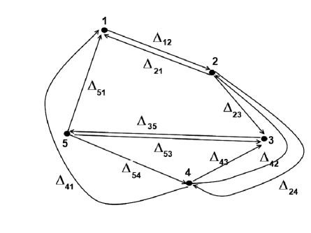
Figure 2: The graph of interactions of a global system of instantaneously coupled units $1,2,\ldots,5$. The oriented and nonzero weighted edges are denoted by $\Delta_{ij}$.

If the interactions weights $\Delta_{i,j}$ are all positive and large enough, the coalition $I(t_{n})$ may be the result of an avalanche process that makes more and more cells spike at the same instant $t_{n}$ when at least one cell spikes. In fact, we can always decompose $I(t_{n})$ as the following union of pairwise disjoint (maybe empty) subsets of cells:

$$I(t_{n})=\bigcup_{p\geq 0}I_{p}(t_{n}),$$

where $I_{0}(t_{n})$ is the set of cells $i$ such that $x_{i}(t_{n}^{-})=\theta_{i}$, and for all $p\geq 1$, the set $I_{p}(t_{n})$ is composed by the cells $j\not\in\cup_{k=0}^{p-1}I_{k}(t_{n})$ such that $x_{j}(t_{n}^{-})+\sum_{k=0}^{k=p-1}\sum_{i\in I_{k}(t_{n})}\Delta_{ij}\geq\theta_{j}.$

Definition 2.4

(Cooperative and antagonist cells)

A cell $i$ is called cooperative if $\Delta_{ij}\geq 0$ for all $j\neq i$. It is called antagonist if $\Delta_{ij}\leq 0$ for all $j\neq i$. It is called mixed if it is neither cooperative nor antagonist.

In Figure 3 we draw the evolution on time of the satisfaction variables of two interacting dynamical units: one of the units is cooperative and the other is antagonist.

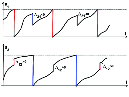
Figure 3: Evolution on time $t$ of the satisfaction variable of two interacting units. One cell is cooperative and the other is antagonist.

From the rule (4), when a cooperative cells spikes, it helps the other cells to increase the values of their respective satisfaction variables, so it shortens the time that the others must wait to arrive to their respective goals. On the contrary, an antagonist cell diminishes the values of the satisfaction variables of the other cells, opposing to them and enlarging the time that the others must wait to arrive to their goals.

Experimentally in Neuroscience, the nervous system of animals rarely show the existence of mixed cells. This is a reason why one usually assumes the so called Dale’s Principle [24, 2]: any cell in the network is either cooperative or antagonist. In [5] abstract mathematical reasons that support Dale’s principle were proved: it is a necessary condition for a maximum dynamical richness in the network. Precisely, the amount of information that the network can exhibit along its temporal evolution in the future acquires its maximum restricted to a constant number of nonzero interactions, only if Dale’s principle holds.

Along this work we focuss on the global dynamics of networks that are composed by cooperative cells and that have a complete graph of interactions.

The global state and the vectorial satisfaction variable

We denote by

$${\bf{x}}(t)=(x_{1}(t),\ldots,x_{m}(t))\in\prod_{i=1}^{m}X_{i}$$

the state of the global system at instant $t\geq 0$. We denote by

$${\bf S}({\bf{x}}(t))=(S_{1}(x_{1}(t)),\ldots,S_{m}(x_{m}(t)))\in\mathbb{R}^{m}$$

the vectorial satisfaction variable of the global system at instant $t$. We consider the cube

$$Q:=\prod_{i=1}^{m}[0,\theta_{i})\subset\mathbb{R}^{m}.$$

From the hypothesis of the free dynamics of the cells and of the mutual interactions, if all the cells are cooperative then

$${\bf S}({\bf{x}}(t))\in Q\ \ \forall\ t\geq 0$$

provided that

$${\bf{x}}(0)\in{\bf S}^{-1}(Q).$$ (5)

Along this paper we will assume condition (5). This assumption is not a restriction for the study of all the orbits of the global autonomous system. In fact, if ${\bf S}({\bf x}(0))\not\in Q$, then, applying the inequality (2) and the reset rule (3, and taking into account that the the interactions are non negative, we deduce that there exists a minimum positive instant $t_{0}$ such that ${\bf S}({\bf x}(t_{0}))\in Q$. So, translating the origin of the time axis to $t_{0}$, we have reduced the problem to the case for which the vectorial satisfaction value initially belongs to $Q$.

Definition 2.5

(Grand coalition) We call $I(t_{n})$, defined in 2.3, the grand coalition if all the cells of the system spike at instant $t_{n}$. Namely, the grand coalition is exhibited at instant $t_{n}$ if $I(t_{n})=\{1,2,\ldots,m\}$.

Definition 2.6

(Waiting time) If from some initial state of the global system the grand coalition is exhibited at some spiking instant $t_{n}\geq 0$, we call the minimum such an instant the waiting time until the grand coalition occurs. Note that in general, if existing, the finite waiting time depends on the initial state.

Weak interactions: We will not need to assume the following condition (6) as an hypothesis. So, it is not an assumption in any part of this paper. Nevertheless, we pose condition (6) just because some of the theorems that we will prove along the work become more interesting for networks that satisfy it:

$$\max_{i\neq j}|\Delta_{ij}|\ll\min_{i}\theta_{i},$$ (6)

where $\ll$ denotes “much smaller than”. For instance, one may be interested in considering $a\ll b$ (where $0<a<b$) if $a/b<10^{-3}$. Condition (6) says that the interactions weights are relatively very weak.

Definition 2.7

(Large networks)

Let $N$ be a network composed by $m$ cooperative units, as described above. We say that $N$ is large enough in relation to the cooperative interactions if the following inequality holds:

$$\sqrt{m}\geq 1+\frac{\max_{i}\theta_{i}}{\min_{i\neq j}\Delta_{ij}}.$$ (7)

Note that, inequality (7) implies that the graph of interactions is complete. In fact $\Delta_{ij}\geq 0$ for all $i\neq j$ because the cells are all cooperative, but

$$\Delta_{ij}\neq 0\ \forall\ i\neq j$$

to make the minimum in formula (7) be nonzero and make this formula hold for a finite value of $m$.

2.2 Statements of the results

The purpose of this paper is to prove the following results:

Theorem 2.8

If the network is cooperative and large enough, then from any initial state the grand coalition is exhibited infinitely many times in the future.

Theorem 2.9

If the network is cooperative and large enough, then from any initial state in ${\bf S}^{-1}(Q)$ the waiting time $t_{n_{0}}$ before the grand coalition appears for the first time is upper bounded by:

$$t_{n_{0}}\leq\max_{i}\ \frac{\theta_{i}}{\min_{x_{i}\in S_{i}^{-1}[0,\theta_{i}]}\bigtriangledown S_{i}(x_{i})\cdot f_{i}(x_{i})}.$$

Theorem 2.10

If the network is cooperative, large enough and if besides all the cells are mutually similar, i.e.

$$\frac{\min_{i}\big{(}{\theta_{i}}/{\max_{x_{i}\in S_{i}^{-1}[0,\theta_{i}]}\bigtriangledown S_{i}(x_{i})\cdot f_{i}(x_{i})}\big{)}}{\max_{i}\big{(}{\theta_{i}}/{\min_{x_{i}\in S_{i}^{-1}[0,\theta_{i}]}\bigtriangledown S_{i}(x_{i})\cdot f_{i}(x_{i})}\big{)}}\geq 1-\frac{\min_{i\neq j}\Delta_{ij}}{\max_{i}\theta_{i}}$$ (8)

then, from any initial state and after a waiting time the grand coalition appears at every spiking instant of the system.

Inequality (8) is satisfied for instance if the cells have mutually identical free dynamics and besides, for each cell $i$, the maximum and minimum velocities $\bigtriangledown S_{i}(x_{i})\cdot f_{i}(x_{i})$ - according to which the satisfaction variable $S_{i}$ increases - are not very different. Hypothesis (8) also holds if the cells are not identical but their differences are small enough so the quotient at left in inequality (8) - which is strictly smaller than 1 - differs from 1 less than $\displaystyle\frac{\min_{i\neq j}\Delta_{ij}}{\max_{i}\theta_{i}}$. If besides the interactions weights $\Delta_{i,j}$ are much smaller than $\theta_{i}$ - cf. condition (6) -, then the similarity among the cells must be very notorious to satisfy the hypothesis of Theorem 2.10.

Roughly speaking, Theorem 2.10 states that if the cells are similar enough then, after a waiting time which depends on the initial state of the global system, the spike of one cell makes all the other cells also spike at the same instant. In other words, the only recurrent coalition is the grand coalition.

3 The proofs

3.1 Proof of Theorem 2.8

Proof: Let $\{t_{n}\}_{n\geq 0}$ the strictly increasing sequence of spiking instants, as defined in 2.2. Let

$$r:=1+\mbox{int}\Big{(}\frac{\max_{i}\theta_{i}}{\min_{i\neq j}\Delta_{ij}}\Big{)},$$

where int denotes the lower integer part. Since by hypothesis the network is large, from Definition 2.7 we obtain:

$$r^{2}\leq m,$$

where $m$ is the number of units in the system.

It said in Section 2, it is not restrictive to assume that the initial state ${\bf x}(0)$ belongs to ${\bf S}^{-1}(Q)$. Thus $S_{i}(x_{i}(0))\in[0,\theta_{i})$ for any unit $i$. We state

Assertion (A) During the time interval $[0,t_{r-1}]$ all the units of the system have spiked at least once.

To prove Assertion (A), let argue by contradiction. Assume that there is a cell, say $j$, such that $x_{j}(t)<\theta_{j}$ for all $t\in[0,t_{r-1}]$. By the interactions rule (4), and since at least one cell spikes at instant $t_{k}$ for all $k=0,\ldots,{r-1}$, we have:

$$S_{j}(x_{j}(t_{r-1}))\geq S_{j}(x_{j}(0))+r\,\min_{i\neq j}\Delta_{ij}\geq S_{j}(x_{j}(0))+\theta_{j}\geq\theta_{j},$$

contradicting the initial assumption. So Assertion (A) is proved.

Now, we state

Assertion (B) If at some instant $t_{n}$ at least $r$ cells spike simultaneously, then all the cells spike simultaneously at $t_{n}$.

To prove Assertion (B) we have, by hypothesis, $\#I(t_{n})\geq r$. Due to the interactions rule (4), for any cell $j\not\in I(t_{n})$ we obtain:

$$S_{j}(x_{j}(t_{n}))\geq S_{j}(x_{j}(t_{n}^{-}))+r\,\min_{i\neq j}\Delta_{ij}\geq\theta_{j},$$

contradicting the assumption that $j\not\in I(t_{n})$. Therefore, all cells are in $I(t_{n})$ proving Assertion (B).

Consider the $r$ coalitions $I(t_{0}),I(t_{1}),\ldots,I(t_{r-1})$. Assertion (A) states that each cell $i$ belongs to at least one of those coalitions. Since the number of different cells is $m\geq r^{2}$, and the number of coalitions in the above list is $r$, there exists at least one of such coalitions, say $I(t_{k})$ having at least $r$ different cells. In other words, there exists a spiking instant $t_{k}$ such that at least $r$ cells spike simultaneously at $t_{k}$. Applying Assertion (B) we deduce that all the cells spike simultaneously at $t_{k}$. We have proved that the grand coalition $I(t_{k})=\{1,\ldots,m\}$ is spontaneously formed at the instant $t^{*}_{0}:=t_{k}>0$. Since this assertion holds for any initial state, we now translate the origin of the time axis to $t^{*}_{0}$, adopting a new initial state from which the grand coalition will be formed again at some future instant $t^{*}_{1}>t^{*}_{0}$. By induction on $n$, the grand coalition will be exhibited recurrently in the future at an increasing sequence of instants $t_{n}^{*}$, ending the proof of Theorem 2.8. $\Box$

3.2 Proof of Theorem 2.9

Proof:

From the proof of Theorem 2.8, the waiting time $t^{*}_{0}$ until the first grand coalition appears is not larger than the instant $t_{r-1}$ such that all the cells have spiked at least once during the time interval $[0,t_{r-1}$. Since all the interactions are positive, $t_{r-1}$ is not larger than the time $T_{i}$ that the slowest cell, say $i$, would take to arrive to its goal $\theta_{i}$ if it were not coupled to the network, i.e. under the free dynamics:

$$t_{0}^{*}\leq t_{r-1}\leq T_{i}.$$

From the relaxation rules (1) and (2) we get

$$\theta_{i}=S_{i}(x_{i}(T_{i}^{-}))=\int_{0}^{T_{i}}\bigtriangledown S_{i}(x_{i}(t))\cdot f_{i}(x_{i}(t))\,dt\geq\Big{(}\min_{x_{i}\in S_{i}^{-1}([0,\theta_{i}])}\bigtriangledown S_{i}(x_{i})\cdot f_{i}(x_{i})\,\Big{)}\,T_{i}$$

Thus

$$t_{0}^{*}\leq T_{i}\leq\frac{\theta_{i}}{\min_{x_{i}\in S_{i}^{-1}[0,\theta_{i}]}\bigtriangledown S_{i}(x_{i})\cdot f_{i}(x_{i})}\leq\max_{i}\ \frac{\theta_{i}}{\min_{x_{i}\in S_{i}^{-1}[0,\theta_{i}]}\bigtriangledown S_{i}(x_{i})\cdot f_{i}(x_{i})},$$

ending the proof of Theorem 2.9. $\Box$

3.3 Proof of Theorem 2.10

Proof:

From Theorem 2.8, there exists a first instant $t_{0}^{*}$ such that the grand coalition is exhibited. From the update rule (3, the state ${\bf x}(t_{0}^{*})$ of the global system is such that ${\bf S}({\bf x}(t_{0}^{*}))={\bf 0}$. We now translate the origin of the time axis to $t_{0}^{*}$. So, the initial state is now ${\bf x}(0)$ such that ${\bf S}({\bf x}(0))={\bf 0}$.

Hence, to prove Theorem 2.10 it is enough to show that, if the hypothesis of inequality (8) holds, then for any initial state ${\bf x}(0)$ such that ${\bf S}({\bf x}(0))={\bf 0}$, all the cells spikes simultaneously at the minimum instant $t_{1}>0$ such at least one cell, say $i$, spikes.

So, let us compute the values of the satisfaction variables of all the cells at the instant $t_{1}^{-}$. Due to the relaxation rules (1) and (2) we have

$$S_{j}(x_{j}(t_{1}^{-}))=\int_{0}^{t_{1}}\bigtriangledown S_{j}(x_{j}(t))\cdot f_{j}(x_{j}(t))\,dt\geq\Big{(}\min_{x_{j}\in S_{j}^{-1}([0,\theta_{j}]}\bigtriangledown S_{j}(x_{j})\cdot f_{j}(x_{j})\Big{)}\ t_{1}\ \ \ \forall\ 1\leq j\leq m.$$ (9)

In particular for the spiking cell $i$ we have

$$\theta_{i}=S_{i}(x_{i}(t_{1}^{-}))=\int_{0}^{t_{1}}\bigtriangledown S_{i}(x_{j}(t))\cdot f_{i}(x_{j}(t))\,dt\leq\Big{(}\max_{x_{i}\in S_{i}^{-1}([0,\theta_{i}])}\bigtriangledown S_{i}(x_{i})\cdot f_{i}(x_{i})\Big{)}\ t_{1}.$$ (10)

Combining inequalities (9) and (10) we deduce:

$$S_{j}(x_{j}(t_{1}^{-}))\geq{\theta_{i}}\ \frac{\min_{x_{j}\in S_{j}^{-1}([0,\theta_{j}])}\bigtriangledown S_{j}(x_{j})\cdot f_{j}(x_{j})}{\max_{x_{i}\in S_{i}^{-1}([0,\theta_{i}])}\bigtriangledown S_{i}(x_{i})\cdot f_{i}(x_{i})}\geq$$

$$\geq\theta_{j}\ \ \frac{\min_{i}\big{(}{\theta_{i}}/{\max_{x_{i}\in S_{i}^{-1}[0,\theta_{i}]}\bigtriangledown S_{i}(x_{i})\cdot f_{i}(x_{i})}\big{)}}{\max_{j}\big{(}{\theta_{j}}/{\min_{x_{j}\in S_{j}^{-1}[0,\theta_{j}]}\bigtriangledown S_{j}(x_{j})\cdot f_{j}(x_{j})}\big{)}}\ \ \ \ \forall\ j\neq i.$$

Using now the hypothesis of inequality (8, we obtain:

$$S_{j}(x_{j}(t_{1}^{-}))\geq\theta_{j}\ \Big{(}1-\frac{\min_{i\neq j}\Delta_{ij}}{\max_{i}\theta_{i}}\Big{)}\geq\theta_{j}-\min_{i\neq j}\Delta_{ij}\ \ \ \ \forall\ j\neq i.$$

Since at least the cell $i$ spikes at instant $t_{1}$ we have

$$S_{j}(x_{j}(t_{1}^{-}))+\sum_{i\in I(t_{1}),\ i\neq j}\Delta_{ij}\geq S_{j}(x_{j}(t_{1}^{-}))+\min_{i\neq j}\Delta_{ij}\geq\theta_{j}.$$

So, applying the interaction rule (4) we deduce that the cell $j$ spikes at instant $t_{1}$. This result holds for all the cells $j\neq i$. Thus, all the cells spike when at least one spikes, ending the proof of Theorem 2.10. $\Box$

Acknowledgement

We thank the scientific and organizing committees of the IV Coloquio Uruguayo de Matemática, for the invitation to give a talk during the event on the subject of this paper.

References

- [1] E. Accinelli, S. London, and E. Sánchez Carrera, A Model of Imitative Behavior in the Population of Firms and Workers, Quaderni del Dipartimento di Economia Politica 554, University of Siena, Siena, 2009
- [2] M.F. Bear, B.W. Connors, M.A. Paradiso: Neuroscience - Exploring the Brain, 3rd. Edi- tion, Lippincott, Williams & Wilkins, Philadelphia, 2007
- [3] S. Bottani, Synchronization of integrate and fire oscillators with global coupling, Physical Review E, 54 (1996), 2334–2350 doi: 10.1103/PhysRevE.54.2334
- [4] J. Bremont, Dynamics of injective quasi-contractions, Erg. Theor. Dyn. Syst. 26 (2006) 19–44
- [5] E. Catsigeras: Dale’s Principle is Necessary for an Optimal Neural Network’s Dynamics Appl. Math. (Irvine)4 (2013) 15–29 doi: 10.4236/am.2013.410A2002
- [6] E. Catsigeras and P. Guiraud Integrate and Fire Neural Networks, Piecewise Contractive Maps and Limit Cycles. Journ. Math. Biol. 67(3), (2013) 609–655, doi: 10.1007/s00285-012-0560-7
- [7] B. Cessac, A discrete time neural network model with spiking neurons. Rigorous results on the spontaneous dynamics, Journ. Math. Biol. 56 (2008) 311–345.
- [8] J.R. Chazottes and B. Fernandez (Eds), Dynamics of coupled map lattices and of related spatially extended systems, Lecture Notes in Physics 671 Springer Berlin, 2005
- [9] R. Coutinho, B. Fernandez, R. Lima and A. Meyroneinc, Discrete time piecewise affine models of genetic regulatory networks, Journ. Math. Biol. 52 (2006), 524-570 doi: 10.1007/s00285-005-0359-x
- [10] G.B. Ermentrout, An adaptive model for syncrhony in the firefly Pteroptyx malaccae Journ. Math. Biol. 29 (1991), pp. 571–585
- [11] G.B. Ermentrout and D.H. Terman, Mathematical Foundations of Neuroscience. Springer, 2010
- [12] J. Feng, L. Zhu and H. Wang, Stability of Ecosystem induced by mutual interference between predators, Procedia Environmental Sciences 2 (2010) 42-48
- [13] E.M. Izhikevich, Dynamical Systems in Neuroscience: The Geometry of Excitability and Bursting. MIT Press, 2007
- [14] N. Jiménez, S. Mihalas, R. Brown, E. Niebur and J. Rubin, Locally contractive dynamics in generalized integrate-and-fire neuron models Preprint Johns Hopkins Univ., Univ. of Pittsburgh and Allen Institute for Brain Science, (2013) http://www.math.pitt.edu/ rubin/pub/pub.html (Last retrieved February 7th., 2013)
- [15] K.K. Lin and L.S. Young, Shear-induced chaos. Nonlinearity 21 (2008) 899–922.
- [16] K.K. Lin, K.C.A. Wedgwood, S. Coombes and L-S Young, Limitations of perturbative techniques in the analysis of rhythms and oscillations, Journal of Mathematical Biology 66 (2013), 139–161
- [17] W. Mass and C.M. Bishop (Eds), Pulsed Neural Networks, MIT Press, Cambridge, 2001.
- [18] I. Milchtaich, Representation of finite games as network of congestion, Int. Journ. Game Theory 42 (2013) 1085–1096 doi: 10.1007/s00182-012-0363-5
- [19] R.E. Mirollo and S.H. Strogatz, Synchronization of pulse-coupled biological oscillators, SIAM J. Appl. Math. 50 (1990) 1645–1662.
- [20] A. Pikovsky and Y. Maistrenko (Editors), Synchronization: Theory and Application, Kluwer Academic Publ, Dordrecht, 2003.
- [21] G.M. Ramírez Ávila, J.L. Guisset and J.L. Deneubourg, Synchronization in light-controlled oscillators, Physica D, 182 (2003) 254–273
- [22] N. Rubido, C. Cabeza, S. Kahan, G.M. Ramírez Ávila and A. C. Marti, Synchronization regions of two pulse-coupled electronic piecewise linear oscillators, Europ. Phys. Journ. D 62 (2011), 51–56 doi: 10.1140/epjd/e2010-00215-4
- [23] G.T. Stamov and I. Stamova, Almost periodic solutions for impulsive neural networks with delay, Applied Mathematical Modelling 31 (2007) 1263–1270
- [24] P. Strata, R. Harvey: Dale’s Principle, Brain Res. Bull. 50 (5-6) (1999) 349–350 doi:10.1016/S0361-9230(99)00100-8
- [25] D.A. Vasseur and J. Fox, Phase-locking and environmental fluctuations generate synchrony in a predator prey community, Nature 460 (2009) Issue 7258, 1007–1010 doi:10.1038/nature08208
- [26] W. Wang and J.J.E. Slotine, On partial contraction analysis for coupled nonlinear oscillators, Biolog. Cybernetics 92 (2005) 38–53
- [27] T. Yang and L.O. Chua, Impulsive stabilization for control and synchronization of chaotic systems: theory and application to secure communication, IEEE Trans. Circuits Syst. 44 (1997), 976–988.
- [28] X. Yang, C. Huang, Q. Zhu, Synchronization of swiched neural networks with mixed delays via impulsive control, Chaos Solit and Frac. 44 (2011), 817–826.