Reconstruction of network structures from repeating spike patterns in simulated bursting dynamics

Abstract

Repeating patterns of spike sequences from a neuronal network have been proposed to be useful in the reconstruction of the network topology. Reverberations in a physiologically realistic model with various physical connection topologies (from random to scale-free) have been simulated to study the effectiveness of the pattern-matching method in the reconstruction of network topology from network dynamics. Simulation results show that functional networks reconstructed from repeating spike patterns can be quite different from the original physical networks; even global properties, such as the degree distribution, cannot always be recovered. However, the pattern-matching method can be effective in identifying hubs in the network. Since the form of reverberations are quite different for networks with and without hubs, the form of reverberations together with the reconstruction by repeating spike patterns might provide a reliable method to detect hubs in neuronal cultures.

I Introduction

One of the most fundamental problems in the understanding of neural networks is to relate the observed dynamics of a network to its connection structure Feldt et al. (2011). Since networks made of similar elements and interactions, such as our brains, can perform seemingly very different tasks, it is believed that the functions of the network are mainly governed by its connection structure not its constituents. In general, the behavior of a network is governed by the dynamics of its individual elements, their interactions and their connection topology Albert and Barabási (2002). It is straight forward to compute the dynamics of the network when all these three factors are known. However, the reverse problem of reconstructing the structure of the network from its dynamics is highly non-trivial Ching et al. (2013). It is possible that different physical connection structures might give rise to similar observed dynamics. Also, the dynamics of a network can be history dependent (memory) without any changes in physical connections.

However, since the physical connection of a neural network is usually not available and the network dynamics is the only information one can obtain from a neural network, many studies have been devoted to the studies of network reconstruction from the observed dynamics; such as cross correlation Pires et al. (2014), Granger causality Granger (1969), transfer entropy Schreiber (2000) etc. Reconstructing the underlying network connection solely from the measurement of the time-series signal of the elements is in general a difficult task, albeit it can be achieved recently for undirected networks of uniform coupling strengths Ching et al. (2013) or for directed networks with loop-free structure Pires et al. (2014). The problem becomes even more challenging for the case of neuronal networks due to the directed synaptic connections and their dynamically dependent plasticity. One intuitively simple attempt for neuronal network reconstruction is based on repeating spatial temporal firing patterns Sun et al. (2010) of the network. In the concept of cell assembly Hebb (1949), proposed by Hebb as a possible mechanism for the realization of higher brain functions from interconnected neurons, these repeating spike patterns are believed to be related to the network connection structure of the cell assembly. One of the earliest attempts for the search of cell assembly Abeles and Gerstein (1988) was to use multi-site recordings of neuronal activities to examine the spatial–temporal firing patterns in cultures and in vivo experiments. In these studies, the repeating spike patterns are considered fundamental because they represent a dynamical characteristic of the network which should be intimately related to its connection structure. Although the relation between these repeating spike patterns and the network structure is still far from clear, one can still “reconstruct” network structures from these pattern, if the notion of “fire together, wire together” is used. With this heuristic rule, repeating spike patterns obtained from neuronal cultures have been used to reconstruct network structures Sun et al. (2010).

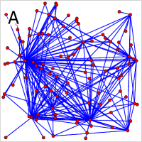
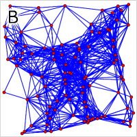
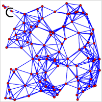
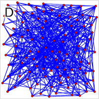
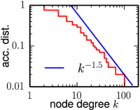
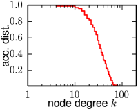
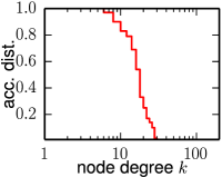
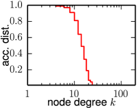
Figure 1: (Color online) Different network structures generated with Morita’s method Morita (2006) with A: $\gamma=1.5$, $\delta=2.7$; B: $\gamma=3$, $\delta=4.7$; C: $\gamma=5$, $\delta=2$; and a random network D with similar degree distribution to C.

One important characteristics of network reconstructed from dynamics is that the reconstructed network structures are only “functional”. Since it is known that even a simple network of cultured neurons can display different kind of dynamics within a short time when drugs Maeda et al. (1995) are added to the perfusion. The functional network deduced from dynamics might not reflect the physical connections in the system. It is not uncommon that different studies of functional networks in the brain can find both scale-free Eguíluz et al. (2005) and small-world Achard et al. (2006) topologies. Presumably, different kinds of functional topologies could be created dynamically from the same physical network. Very little is known about the relation between the functional network and its physical counter part. It would be desirable if there were control experiments in which both the physical connection and resultant dynamics are known so that we can study the relation between the the functional network and the physical network. Unfortunately, these ideal experiments do not exist yet. As a remedy for such a situation, computer simulations might be useful. In this article, we describe our studies on the relation between the physical network and its reconstructed functional network from repeating spike patterns in the simulation of a physiologically realistic model Volman et al. (2007) which is known to reproduce reverberations found in experiments Lau and Bi (2005). Our results suggest that the method of repeating spike patterns might be useful for the local reconstruction of hubs during reverberation if hubs exist. However, as global structure is concerned, such as the degree distribution, the repeating-spike-pattern method might not be applicable.

II Methods

Our simulation studies of relation between physical networks and function networks are consisted of three main steps; namely a) network generation, b) simulation of network dynamics and c) functional-network reconstruction. We use a network generation method in which the topologies of the network can be changed continuously from random to scale free by tuning some system parameters. This flexibility will allow us to use the same structure generation algorithm for various topologies and more importantly to generate structures in between random and scale free. For the network dynamic simulation, a physiologically realistic model is chosen. The model is known to be able to generate reverberation patterns similar to experimental observations in neuronal cultures Lau and Bi (2005). As for the functional network reconstruction, we use the repeating-spike-pattern method which have been used to identify network topologies in neuronal cultures. Details of these three steps are given below.

II.1 Network Generation

In order to generate networks of different structures, we used the method described by Morita Morita (2006); Gosak et al. (2010). In this method, $N$ vertices of the network are distributed randomly on a 2D unit square. Two vertices $i$ and $j$ are connected if their locations satisfy the equation,

$$\frac{2l_{i,j}^{2}}{a_{i}a_{j}}<\delta,$$ (1)

where $l_{i,j}$ is the distance between the two points, $\delta$ is a threshold parameter, and $a_{i}=\left(i/N\right)^{1/\left(1-\gamma\right)}$ for a given parameter $\gamma>1$. A main advantage of Morita’s method is that different types of network topology can be generated by continuous changes of the parameters $\gamma$ and $\delta$. Figure 1 shows three network structures generated with different parameters in Morita’s method along with a Erdős–Rényi random network Erdős and Rényi (1959) as well as their corresponding accumulative degree ($k$) distributions. From the left, the degree distributions of the networks in Fig. 1 range from scale free with a power of $-2.5$ to Gaussian-like similar to the random network. Beside being tunable in their degree distributions, the networks generated with Morita’s method are also pertinent to a 2D geometry, similar to a neural culture, which is apparent when comparing the last (third from the left) network structure to the random network with similar degree distribution on the right of Fig. 1: The vertices that are closer to each other in the geometrical space are more likely to be connected.

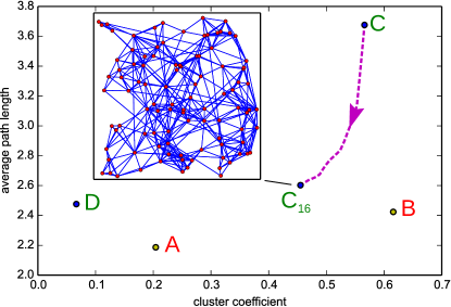
Figure 2: (Color online) Average path lengths versus cluster coefficients for the networks A to D as shown in Fig. 1. Network ${\rm C}_{16}$, as shown in inset, is network C with 16 pairs of links rewired to minimize average path length while preserving the degree structure for all the nodes. It represents a small-world construction from the geometrically constrained network C.

Following recent findings of small-world Watts and Strogatz (1998) structures in cultured networks Downes et al. (2012); de Santos-Sierra et al. (2014), we calculate the cluster coefficients as well as average path length between nodes for the networks in Fig. 1 and plot them as labeled in Fig. 2. Similar to the lattice based regular network in Watts and Strogatz (1998), the network C has a large cluster coefficient and relatively long average path length since it is similarly constrained to a geometric space while connections are short-ranged. We perform pair-rewiring steps similar to that described in Maslov and Sneppen (2002) to minimize the average path length of C while preserving its degree distribution. The network ${\rm C}_{16}$ as depicted in the inset of Fig. 2, arrived after 16 pair-rewiring steps, has an average path length on par with random network D while maintaining about 80% of its cluster coefficient. We consider network ${\rm C}_{16}$ as a small-world intermediate between networks C and D.

In the following analysis, we will limit our consideration to the five different networks, each of 100 neurons, as shown in Fig. 1 and Fig. 2 with bidirectional connectivity.

II.2 Model of network dynamics

The notion of “fire together wire together” has been used in many studies to identify functional connection in cultures. Usually, “fire together” can mean strong correlation or even synchronization. It is well known that neuronal cultures develop synchronized bursting during development although its origin is still not clear. In a study of using core patterns to identify connection during development, Sun et al Sun et al. (2010) have also used the repeated spike patterns in synchronized bursts to identify connections. Here, our simulation is based on a recent model by Volman et al Volman et al. (2007) describing the dynamics of reverberation activity in cultured neural networks in which synchronized bursts have been observed. In this model, the dynamics of neurons follows the Morris–Lecar model Morris and Lecar (1981); Rinzel and Ermentrout (1989),

$$C\frac{dV}{dt} = -I_{{\rm ion}}+G\left(V_{r}-V\right)+I_{{\rm bg}},$$ (2a)

$$\frac{dW}{dt} = \theta\frac{W_{\infty}-W}{\tau_{W}}$$ (2b)

where

$$I_{{\rm ion}}=g_{{\rm Ca}}m_{\infty}\left(V-V_{{\rm Ca}}\right)+g_{{\rm K}}W\left(V-V_{{\rm K}}\right)+g_{{\rm L}}\left(V-V_{{\rm L}}\right)$$ (3)

is the current through the membrane ion channels,

$$\tau_{W} = \left(\cosh\frac{V-V_{3}}{2V_{4}}\right)^{-1},$$ (4a)

$$W_{\infty} = \frac{1}{2}\left(1+\tanh\frac{V-V_{3}}{V_{4}}\right),$$ (4b)

$$m_{\infty} = \frac{1}{2}\left(1+\tanh\frac{V-V_{1}}{V_{2}}\right)$$ (4c)

are the voltage dependent dynamic parameters, and the threshold $V_{{\rm th}}$ of membrane potential defines the spiking events which result in synchronous releases of neural transmitters at the efferent synapses. Additionally, a residual calcium variable $R_{{\rm Ca}}$ driven by the spiking events,

$$\frac{d}{dt}R_{{\rm Ca}}=\frac{-\beta R_{{\rm Ca}}^{n}}{k_{R}^{n}+R_{{\rm Ca}}^{n}}+I_{p}+S\gamma\log\frac{R_{{\rm Ca}}^{0}}{R_{{\rm Ca}}},$$ (5)

where the spike train $S=\sum_{\sigma}\delta\left(t-t_{\sigma}\right)$ with $t_{\sigma}$ being the time of the spike event $\sigma$, is used to determine the rate,

$$\eta=\eta_{{\rm max}}\frac{R_{{\rm Ca}}^{m}}{k_{a}^{m}+R_{{\rm Ca}}^{m}},$$ (6)

of synapse-dependent asynchronous releases following an independent Poisson process at each efferent synapse. The neural transmitters released by the spike-driven synchronous and calcium-dependent asynchronous events follow a four-state decaying dynamics based on a modification of the Tsodyks–Uziel–Markram (TUM) model Tsodyks et al. (2000),

$$\frac{dX}{dt} = \frac{Q}{\tau_{s}}+\frac{Z}{\tau_{r}}-uXS-X\xi$$ (7a)

$$\frac{dY}{dt} = -\frac{Y}{\tau_{d}}+uXS+X\xi$$ (7b)

$$\frac{dZ}{dt} = \frac{Y}{\tau_{d}}-\frac{Z}{\tau_{r}}-\frac{Z}{\tau_{l}}$$ (7c)

$$\frac{dQ}{dt} = \frac{Z}{\tau_{l}}-\frac{Q}{\tau_{s}}.$$ (7d)

where $\xi=\bar{\xi}\sum_{a}\delta\left(t-t_{a}\right)$ summing over asynchronous release event $a$ with Poisson rate given by (6), to include a super-inactive state $Q$ Volman et al. (2007). Multiplying by the synaptic weights, the fractions of neural transmitters in the active state $Y$ (7b) determine the contribution of the afferent synapses to the membrane conductance $G$ of a post-synaptic neuron through a linear sum

$$G_{i}=\sum_{j}w_{ji}Y_{ji}$$ (8)

over all pre-synaptic neurons $j$ of a given post-synaptic neuron $i$. Following Volman et al. (2007), the synaptic weights $w$ are randomly drawn from a truncated Gaussian distribution with a width that is $\pm 20\%$ of its mean $\bar{w}$. The super-inactive state $Q$ (7d) of neural transmitters plays a part in taking up neural transmitters during a burst of reverberations and eventually terminates the reverberatory burst.

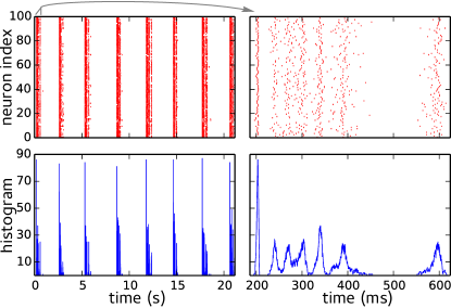
Figure 3: (Color online) Typical bursting behavior of a random network (D in Fig. 1) with neuron and synaptic transmission models described in Volman et al. (2007). The left panels show eight bursts for a duration of about 20 seconds while the right panels are the zoom-in on the first burst. The upper panels are the raster plots marking the spiking events for the neurons indexed on the vertical axes. The bottom panels are histograms with the vertical axis showing the number of spikes within a sliding bin of 4 ms.

In this model, there are two types of noises. The first one is the background current $I_{{\rm bg}}$ which is uniformly added to every neuron to mimic a noisy environment. The other is the asynchronous release due to the residual calcium in the neuron after firing. The latter types of noise can be considered a kind of short term memory because it is related to the firing history of the neuron. The Poisson processes modeling these asynchronous events are the only sources of stochasticity in the model. A typical bursting state of the system is shown in Fig. 3 with sub-burst reverberations. Notice that in Volman et al. (2007), the reverberatory burst was triggered by an external stimulus while spontaneous bursting is possible but rare. This corresponds to the regime of high to infinite restitution ratio in our cases where the networks will be silent by themselves.

Note that the chosen residual calcium dynamics and the synaptic mechanisms are responsible for the reverberation (bursts) shown in Fig. 3. The dynamics of the network depends on the parameters of the model as well as the network topology. As there are a total of 30 parameters used from (2) to (7) to define the model in Volman et al. (2007), we do not intend to be comprehensive in exploring the entire phase space.

Table 1: Values of fixed model parameters

Morris–Lecar model
$V_{{\rm Ca}}$	$100$ ${\rm mV}$	$V_{2}$	$15$ ${\rm mV}$	$g_{{\rm L}}$	$0.5$ ${\rm mS}$
$V_{{\rm K}}$	$-70$ ${\rm mV}$	$V_{3}$	$0$ ${\rm mV}$	$C$	$1$ ${\rm\mu F}$
$V_{{\rm L}}$	$-65$ ${\rm mV}$	$V_{4}$	$30$ ${\rm mV}$	$\theta$	$0.2$ ${\rm ms}^{-1}$
$V_{r}$	$0$ ${\rm mV}$	$g_{{\rm Ca}}$	$1.1$ ${\rm mS}$	$V_{{\rm th}}$	$10$ ${\rm mV}$
$V_{1}$	$-1$ ${\rm mV}$	$g_{{\rm K}}$	$2$ ${\rm mS}$

TUM synaptic transmission
$\tau_{d}$	$10$ ${\rm ms}$	$\tau_{l}$	$600$ ${\rm ms}$	$u$	$0.2$
$\tau_{r}$	$300$ ${\rm ms}$	$\tau_{s}$	$5000$ ${\rm ms}$	$\bar{\xi}$	$0.02$

Residual calcium dynamics
$\beta$	$0.005$ $\frac{{\rm\mu M}}{{\rm ms}}$	$\gamma$	$0.033$	$k_{a}$	$0.1$ ${\rm\mu M}$
$k_{R}$	$0.4$ ${\rm\mu M}$	$R_{{\rm Ca}}^{0}$	$2000$ ${\rm\mu M}$	$m$	$4$
$I_{p}$	$1.1\times 10^{-4}$ $\frac{{\rm\mu M}}{{\rm ms}}$	$\eta_{{\rm max}}$	$0.32$ ${\rm ms}^{-1}$	$n$	$2$

Instead, we fix all parameters with values shown in Table 1, similar to what were documented in Volman et al. (2007), except for the background current $I_{{\rm bg}}$ and mean synaptic weight $\bar{w}$, which are varied to obtain a network with spontaneous bursting behavior. Since the reverberations reproduced in this model with a random network are consistent with those found in experiments Volman et al. (2007), presumably the simulations we carry out here with different topologies are physiologically realistic.

II.3 Repeating-spike-pattern detection

We follow the method in Sun et al. (2010) to use repeating spike patterns for the reconstruction of the network in our simulation. Briefly, repeating spike patterns are defined as repetitive patterns of a sequence of firings from different neurons and a link is assigned between two neurons (wire together) if the spikes of these two neurons are linked in time (fire together). To detect repeating spike patterns, a template-matching algorithm following Rolston et al. (2007) were implemented to locate the repetitive firing patterns among these spiking data to form the repeating patterns.

Since the repeating spike patterns are assumed to have linear connections with only links between adjacent neurons in the spike-time sequenceSun et al. (2010), this reconstruction method ignores the possibility of “branching” in the propagation of spiking activity and could likely predict some connections that were not present in the actual network structure. Note that in Sun et al. (2010), spike sorting was needed to produce a vector of spike times for each identified neuron from the time series recorded by a multi-electrode array. In our case, since all the neurons are known, no spike sorting is needed and only spike detection is performed to produce the spike-time vector. In the current study, a similar MATLAB code as that was used in Sun et al. (2010) is applied to the spiking data generated by the dynamics in II.2 on the networks described in II.1 to find repeating spike patterns for the systems.

III Results

With the methods described above, it is obvious that for a network with fixed topology, the dynamics of the network can be strongly dependent on the choice of synaptic strength and the background current. If we want to reconstruct the topology of the network from the dynamics, we would like to create a situation in which the simulation results will be similar to those in experiments. It is known that synchronized bursting activities emerge as cortical neuronal cultures develop and the network connectivity increases Jia et al. (2004); Lai et al. (2006). As mentioned earlier, for a developing neural cultures, repeating spike patterns will appear during spontaneous bursting. Thus, our goal is to reproduce spontaneous bursting as in Sun et al. (2010). In the original model, the background current is chosen in such a way that the network is in a quiescent steady state in the absence of input but would produce a single, reverberatory burst after an excitatory current is presented to one of the neuron in the network Volman et al. (2007). Since we would like to compare with Sun et al. (2010), we need to adjust the background current to give spontaneous, synchronized bursting. Such spontaneous burst will be followed by a quiescent state. In experiments, the durations of the quiescent state decrease as the culture mature while the durations of the bursting also decrease but less significantly. In the simulation, we can use the ratio between these two states as an indication of the age of the culture. For a fixed background current, this ratio can be tuned by the synaptic strength.

To define the bursting state of the network in our simulation, we use a hysteretic criteria: the system is considered to enter bursting/resting state when there have been more/less than nine/three distinct neurons firing spikes within last 200 ms time window. These numbers are chosen to be similar to those in real experiments. With the defined states, we can measure the durations of bursting and resting episodes. In simulations, for a given background current $I_{{\rm bg}}$ ranging from $27.0$ to $29.5$ $\mu$A, we adjust the the mean synaptic weight $\bar{w}$ of the network to obtain bursting behavior similar to what is shown Fig. 3.

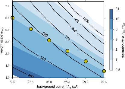
Figure 4: (Color online) Phase diagram for bursting dynamics on a random network. Colors (shades of gray) indicate the restitution ratio of bursting while labeled lines show the average bursting period in milliseconds.

For further pattern matching, we choose the mean synaptic weight so that the ratio between average durations of resting to bursting states (restitution ratio) is 3 to 1 rat as indicated by circles in Fig. 4. Since $I_{{\rm bg}}$ determines how easily a neuron is ready to fire while $w_{{\rm scale}}$ determines how strongly a neuron’s firing can influence others, one would expect an increase in $I_{{\rm bg}}$ would be compensated by a decrease of $w_{{\rm scale}}$. From our simulations, this trend can be more or less observed for networks with more uniform, Gaussian degree distribution (network C and D in Fig. 1 as well as ${\rm C_{16}}$ in Fig. 2). In the following, we report the results of our simulation with the parameters given in Table 1 while the background current $I_{{\rm bg}}$ and mean synaptic weight scale $w_{{\rm scale}}$ being adjusted to give the restitution ratio of 3 to 1.

III.1 Bursting behavior

For each of the networks given in Fig. 1, we perform simulations to obtain spontaneous bursting by varying the background current $I_{{\rm bg}}$ and mean synaptic weight scale $w_{{\rm scale}}$.

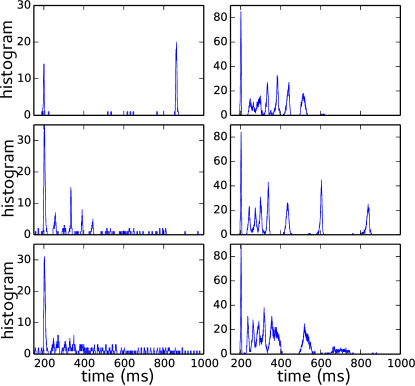
Figure 5: (Color online) Comparison of bursting behavior for scale-free network A (left) with random network D (right) in Figure 1 at three different background current: from top down $I_{{\rm bg}}$ = $27.5$, $28.5$, $29.5$ $\mu A$. The horizontal axes measure time in milliseconds while the vertical axes show the number of spikes within a 4 ms sliding window.

Figure 5 are the typical results for spontaneous bursting for a scale-free and a random network. It can be seen from Fig. 5 that the main difference in the firing patterns between a random network and a scale-free network is the reverberations within the synchronized bursts of random network and their absence in the scale-free network. This difference in bursting behavior is probably due to the existence of hub neurons in the scale-free network which are found to stay active the entire time for any reasonable choices of $I_{{\rm bg}}$ and $w_{{\rm scale}}$ that allow for other neurons in the network to be activated. This constant activation disrupts the quiescence between the reverberations and breaks the coordinated firing of neurons required by the reverberation. The situation is especially true for cases of lower background current where stronger synaptic weights are required. This is one of the reasons that we adopted the hysteretic criteria described in III to define the bursting/resting states of the systems.

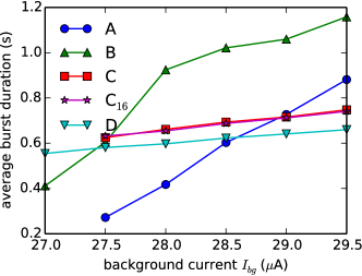
Figure 6: (Color online) Average burst durations when mean synaptic weights of a network is adjusted to have 3-to-1 rest-to-burst duration ratio for the networks given in Fig. 1 and Fig. 2 as functions of the background current given in the model.

The qualitative change of bursting behavior with different network topologies can also be seen in the dependence of the mean burst duration on $I_{{\rm bg}}$ as shown from Fig. 6. It can be seen in Fig. 6 that the burst duration of networks with narrow degree distribution, such as C, ${\rm C}_{16}$, and D, are insensitive to $I_{{\rm bg}}$ when compared to networks with boarder degree distribution, such as A and B. Beside the dependence of burst duration on $I_{{\rm bg}}$, we note there are significantly less reverberations (repeated rises of system activity level, as can be seen in left panel of Fig. 3) within a burst for scale-free network A. It is less so for network B where the reverberations are quite evident in the mid-range of background current Sup . The insensitivity of burst duration on $I_{{\rm bg}}$ for networks C, ${\rm C}_{16}$, and D in Fig. 6 shows the equivalence of excitability of neurons and efficacy of synapses in networks of narrow degree distributions. Both of the networks also retain clear reverberatory behavior for the entire range of background current we considered Sup .

III.2 Properties of repeating spike patterns

With time series similar to those from Figure 5 for all the neurons in the networks, the template-matching method in Sun et al. (2010) is used to identify repeating spike patterns. Data sets corresponding 8 bursting events of the networks are used for repeating-spike-pattern identifications. This amounts to about 3000 spikes per data set, similar to what was considered in Sun et al. (2010) limited by the computer capability for the algorithm used. While more patterns will generally result from a larger data set, we do not expect a qualitative change to our conclusions presented below Sup . Each identified repeating spike pattern is cross-checked with the original network used in the simulation to see if: a) the nodes in the pattern form a connected subnetwork with the original links and b) the nodes in the identified repeating spike pattern are actually connected sequentially in the nominal network as suggested in Sun et al. (2010).

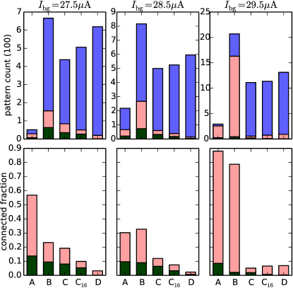
Figure 7: (Color online) The number of repeating spike patterns identified from spiking data of 8 bursts for the five networks in Figs. 1 and 2 for different levels of background current. Blue (full) bars in top panels are the total numbers of identified patterns from the code in Sun et al. (2010). Pink (light gray) bars are for the number of identified patterns that form a connected subnetwork in the original nominal networks used to generate the spiking data. Green (dark) bars are for the number of patterns whose neurons are actually connected following the same sequence of spike times in each pattern. The upper panels show the number of patterns in unit of hundreds while the lower panels show the fractions of connected patterns relative to the total number detected.

Figure 7 shows the results of the statistics of the identified repeating spike patterns for these two properties. A remarkable feature of Fig. 7 is that the number of detected repeating spike patterns are high in networks with narrow degree distributions (C, ${\rm C}_{16}$, and D). That is: repeating spike patterns are more frequent in network with narrow degree distribution. Unfortunately, most of the detected patterns are consisted of nodes that do not form a connected subnetwork in the original network. These repeating spike patterns will give erroneous results if they are used for the reconstruction of the original network.

Furthermore, for those patterns with nodes forming a connected subnetwork, only a small fraction of them are actually linked sequentially following the spike-time orders in the patterns. On the other hand, although there are far less repeating spike patterns detected for the scale-free network A, a much more significant fraction of these patterns are actually consisted of nodes forming connected subnetwork in the original nominal networks; especially for higher background current $I_{{\rm bg}}=29.5$ $\mu$A. It can be seen from Fig. 7 that the connected fraction of detected patterns for the scale-free network seems to be smallest at $I_{{\rm bg}}=28.5$ $\mu$A. This is mainly due to the peaking of spurious patterns since the number of connected patterns decreases monotonically with $I_{{\rm bg}}$.

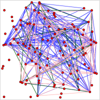
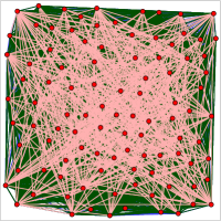
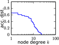
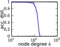
Figure 8: (Color online) Structures of the reconstructed networks (upper panels) from dynamics of scale-free network A (left) and random network D (right) as well as their corresponding degree distributions (lower panels). The links colored in pink (light gray), green (dark), and blue (medium gray) are respectively constructed from patterns of length $\leq 8$, $>32$, and otherwise.

Based on the repeating spike patterns identified, we can follow the method in Sun et al. (2010) to obtain the reconstructed functional network for the four cases as shown in Fig. 8. It can be seen from the figure that the physical connection of the functional network is not only quite different from the physical network, but global property such as the degree distribution of the functional network is also not similar to the physical network.

IV Discussions

From the results obtained above, it is clear that functional networks reconstructed from repeating spike patterns can be quite different from the original physical network. The major reason is that branching in the propagation of neural activity is ignored in our method of reconstruction Sun et al. (2010) with the “fire together wire together” heuristic rule. In our simulations, branching is actually quite important in all the networks studied here. This has actually been considered by Izhikevich Izhikevich (2006) in the so called polychronization of spiking activity. Therefore, we have adopted a relaxed criteria to assess the correlation between the repeating spike patterns and the nominal network structures based on whether the nodes participated in a repeating spike pattern form a connected subnetwork. This is the minimal requirement for a spanning tree to exist on the nominal network that connects all the firing nodes of a repeating spike pattern. We note that, this does not imply that patterns fail to be connected are completely fallacious since some key nodes could have been left out due to numerical error in the template-matching algorithm. In the current study, we do not further investigate how the nominal network structure underlying a repeating spike pattern can be recovered from the spike pattern itself.

Also, we have shown (Fig. 7) that the effectiveness of using the repeating spike patterns to reconstruct the underlying nominal network structure is strongly dependent on the topology of the underlying network and the operating conditions when the spikes are generated. One major difference between a scale-free network and a random network is the existence of well-connected hubs. These hubs can play important roles in relaying information and instigate or modulate activities of the system Bak (1999). A possible reason for the higher fractions of connected repeating spike patterns found for the scale-free A and intermediate B networks is that the high degree of connectivity for these hubs helps the repeating spike patterns they participated in form connected subnetworks of the systems.

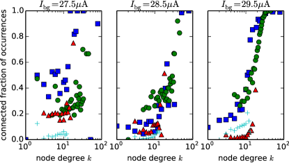
Figure 9: (Color online) Mean fractions of node occurrences in detected patterns that are connected as functions of node degrees. The four different networks are represented by different symbols: A: squares, B: circles, C: triangles, D: pluses.

To verify this hypothesis, we plot in Fig. 9 the mean fractions of a node’s occurrences in repeating spike patterns that form connected subnetworks versus the degree of the node. It is evident from Fig. 9 that patterns of a node with higher degree are more likely to be connected and the highly connected hub nodes in networks A and B are indeed responsible for the high fractions of connected patterns. For larger background current, there exists a degree threshold $k_{c}\approx 30$ above which, all patterns participated by such a node are connected. Such threshold is not clearly evident for lower background current where the synaptic weights are stronger to compensate the lower excitability of neurons.

In our simulations, we find that some of the repeating spike patterns can be embedded into other repeating spike patterns; especially those with short sequence lengths. That is, these repeating spike patterns are subsequences of other repeating spike patterns. These repeating spike patterns are defined as core patterns in Sun et al. (2010) and are thought to be more relevant to the underlying structure of the network. However, we find that in a typically simulations, less than 10% of all the detected repeating spike patterns are core patterns by the criteria in Sun et al. (2010) and only a small number of nodes in the network will take part in these core patterns; especially for network C and D Sup . If we apply our analysis by using core patterns, nodes participated in the core patterns do have a higher fraction to be connected except for the random network D, and the break down to node degree also shows sharper transitions than those shown in Fig. 9 for core patterns Sup . It is still not clear whether the repeating spike patterns or the core patterns are better suited for network reconstruction. Presumably, the core patterns are controlled by the “core nodes” which are likely the hubs in the network while almost all nodes in the network can participate in the repeating spike patterns as long as excitation (noise) in the system is strong enough. In this aspect, the repeating spike patterns should be more relevant in providing information for the reconstruction of the network topology.

The effects of hubs on functional reconstruction can also be seen in the intermediate networks. The network B in Fig. 1 represents an intermediate case between scale-free network with power-law tail in the degree distribution and a more uniformly connected network with Gaussian degree distribution. While there are still a number of hub neurons in such a network, their degrees are limited comparing to the case of scale-free network. Consequently, unlike the scale-free network, all neurons can stop firing during the resting period of its dynamics. We see clear reverberatory bursts in the mid range of background current $I_{{\rm bg}}=28.0\sim 29.0$ $\mu$A Sup . Applying the template-matching method, the spiking dynamics of such a network produces the largest numbers of repeating spike patterns in all conditions studied here. Similar to scale-free network A, the number of connected patterns increases consistently with an increase of background current. Still, only a small fraction of the patterns are actually connected sequentially following their spike times. The picture emerges from our simulations is that although the functional network reconstructed from repeating spike patterns can be quite different from the underlying physical network and even the degree distribution recovered can be quite different, the repeating-spike-pattern method can be effective in identifying hubs when hubs exist. Since the form of reverberations are quite different for networks with and without hubs (Fig 5), the form of reverberations together with the reconstruction by repeating spike patterns might provide a reliable method to detect hubs in the neuronal cultures.

In the current setup, the characteristics of detected repeating spike patterns in the small-world network ${\rm C}_{16}$ seem to well interpolate that of the geometrically constrained network C and random network D. The low fractions of connected patterns can be correlated with the absence of hubs in these networks following the discussion above. There is a steady increase in the number of detected patterns as a geometrically constrained network becomes more random by rewiring. However, the number of these patterns that form connected subnetworks of the underlying nominal network actually becomes less as more links are rewired. While the rewired long links introduce more possibilities for activity propagation, hence more patterns, the neighborhood, cluster structure for a geometrically constrained network can make it more likely for an identified repeating spike pattern to be connected. We note that for the networks of 100 neurons in the current study, the difference in path lengths is very limited for typical consideration of small-world networks. While our results provide a hint on what can be expected, to properly address the small-world effect in repeating spike patterns of simulated neuron networks, significant computing resources need to be invested to consider networks of higher orders of magnitudes in sizes.

Since functional networks reconstructed from repeating spike patterns are governed by both the topology and dynamics of the network and their excitations are the outcome of collective dynamics of the system, perhaps the functional network structure is more relevant to the concept of cell assembly. In fact, Hebb Hebb (1949) had used the phrase “functional unit” when he referred to connections in a cell assembly. In this sense, the repeating spike patterns provide a convenient way to look at the complexity of the system. While their correspondence to the underlying structure of the network can be complicated by various factors as we have shown in the current study, they are perhaps more relevant to the functional dynamics of the network that might serve to fulfill certain biological purposes. The situation is somewhat similar to relating the gene expression in a cell with the primary structure of its DNA sequence. Recently, a novel method Pires et al. (2014) based on covariance and time delay is used to extract the functional connection between different astrocytes during the propagation of ${\rm Ca}^{2+}$ waves induced by an external stimulation. However, this method probably cannot be applied to the case of spontaneous reverberations studied here because in order for the method in Pires et al. (2014) to work, special constrains are introduced for the network reconstruction. These constrains are related to single source of stimulation and the directional nature of the ${\rm Ca}^{2+}$ wave propagation (time delay). In the case of spontaneous reverberations, both of these features are absent. In this work, we studied only spontaneous network dynamics. Similar methods of pattern matching have been used successfully in the identification of functional unit by using evoked activities. In our current study, the excitations for the networks are provided by noise. If some of the nodes in the nominal networks are used as inputs, our simulation method can also be used to study the repeating spike patterns in evoked activities.