Better Optimism By Bayes: Adaptive Planning with Rich Models

Abstract

The computational costs of inference and planning have confined Bayesian model-based reinforcement learning to one of two dismal fates: powerful Bayes-adaptive planning but only for simplistic models, or powerful, Bayesian non-parametric models but using simple, myopic planning strategies such as Thompson sampling. We ask whether it is feasible and truly beneficial to combine rich probabilistic models with a closer approximation to fully Bayesian planning.

First, we use a collection of counterexamples to show formal problems with the over-optimism inherent in Thompson sampling. Then we leverage state-of-the-art techniques in efficient Bayes-adaptive planning and non-parametric Bayesian methods to perform qualitatively better than both existing conventional algorithms and Thompson sampling on two contextual bandit-like problems.

As computer power increases and statistical methods improve, there is an increasingly rich range and variety of probabilistic models of the world. Models embody inductive biases, allowing appropriately confident inferences to be drawn from limited observations. One domain that should benefit markedly from such models is planning and control — models arbitrate the exquisite balance between safe exploration and lucrative exploitation.

A general and powerful solution to this balancing act involves forward-looking Bayesian planning in the face of partial observability, which treats the exploration-exploitation trade-off as an optimization problem, squeezing the greatest benefit from each choice. Unfortunately, this is notoriously computationally costly, particularly for complex models, leaving open the possibility that it might not be justified compared to heuristic approaches that may perform very similarly at a much reduced computational cost, for instance treating the tradeoff as a learning problem in a regret setting, focusing on an asymptotic requirement to discover the optimal solution (to avoid accumulating regret).

The motivation for this paper is to demonstrate the practical power of Bayesian planning. We show that, despite the arduous optimization problem, sample-based planning approximations can excel with rich models in realistic settings – here a challenging exploration-exploitation task derived from a real dataset (the UCI ’mushroom’ task) – even when the data have not been generated from the prior. By contrast, we show that the benefits of Bayesian inference can be squandered by more myopic forms of planning — such as the provably over-optimistic Thompson Sampling – which fails to account for risk in this task and performs poorly. The experimental results highlight the fact that the Bayes-optimal behavior adapts its exploration strategy as a function of the cost, the horizon, and the uncertainty in a non-trivial way. We also consider an extension of the model to a case of more general subtasks, including subtasks that are themselves small mdps (in the suppl. material, Section S4).

The paper is organized as follows: first, we discuss model-based Bayesian reinforcement learning (RL), outline some existing planning algorithms for this case and show why Thompson sampling’s over-optimism can be deleterious. Next, we introduce an exploration-exploitation domain that motivates a statistical model for a class of mdps with shared structure across sequences of tasks. We provide empirical results on a version of the domain that uses real data coming from a popular supervised learning problem (mushroom classification) along with a simulated extension. Finally, we discuss related work.

1 Model-based Bayesian RL

We consider a Bayes-Adaptive planner (?), which starts with a prior $P(\operatorname{\mathcal{P}})$ over models of the environmental dynamics, progressively receives data $\operatorname{\mathcal{D}}$ through controlled interaction with the environment, and updates its posterior distribution over models using Bayes-rule $P(\operatorname{\mathcal{P}}|\operatorname{\mathcal{D}})\propto P(\operatorname{\mathcal{D}}|\operatorname{\mathcal{P}})P(\operatorname{\mathcal{P}})$. Actions are intended to maximize an expected discounted return criterion $\operatorname{\mathbb{E}}[\sum_{t=0}^{\infty}\gamma^{t}r_{t}]$, where $\gamma<1$ is the discount factor and $r_{t}$ is the random reward obtained at time $t$. In an uncertain world, this requires balancing exploration and exploitation. Here, the discount factor $\gamma$ plays the crucial role of arbitrating the relative importance of future rewards. In general, a low $\gamma$ does not warrant much exploration because future exploitation will be heavily downweighted. The opposite is true as $\gamma\rightarrow 1$. A clear illustration of these $\gamma$-dependent exploration-exploitation Bayesian policies can be found in the Gittins indices (?).

The (Bayes-)optimal strategy integrates over how the current belief $P(\operatorname{\mathcal{P}}|\operatorname{\mathcal{D}})$ could be transformed in the light of (imaginary) possible future data. The resulting policy is well known to be the solution to an augmented Markov Decision Process (mdp), whose details we defer to the suppl.  material, Section S1. Finding the exact Bayes-optimal policy is computationally intractable even for tiny state spaces, since (a) the augmented state space is either continuous or discrete and potentially unbounded; and (b) the transitions of the augmented mdp require integration over the full posterior. Although this operation can be trivial and closed-form for some simple probabilistic models (e.g., independent Dirichlet-Multinomial), it is intractable for most rich models.

A common solution to (b) is to use approximate inference methods, such as Markov chain Monte Carlo (mcmc). This fits snugly with a common heuristic for (a), in which the planning problem is side-stepped by sampling from the posterior but only planning myopically. We describe one such method called Thompson Sampling in the section below, but show that it is no panacea.

A potentially more powerful class of approximate solutions to (a) that should be capable of handling large state spaces and complex models involves sample-based forward-search methods. Algorithms such as Sparse Sampling (?) or bamcp (?) do not plan myopically; they approximate Bayes-adaptive planning directly — albeit at a computational cost. It had been unclear how to integrate these methods with approximate, mcmc, approaches to (b). However, recent algorithmic developments (?) provide a practical way to use approximate inference schemes to perform sample-based planning with sophisticated models.

1.1 Thompson Sampling

Thompson Sampling (ts) (?) is a myopic planning method that selects actions at each step by 1) drawing a single sample of the dynamics from the posterior distribution $P(\operatorname{\mathcal{P}}|\operatorname{\mathcal{D}})$ ; 2) greedily solving the corresponding sampled mdp; and 3) choosing the optimal action of this mdp at the current state. Though heuristically myopic from the perspective of Bayes-adaptivity, ts is computationally cheap, and has been proven both empirically (?) and theoretically to perform well in various domains (including reaching theoretical regret lower-bounds for multi-armed bandits (?)). As mentioned, it fits well with complex, e.g., Bayesian non-parametric, models that in any case are handled via mcmc sampling (?).

Intuitively, ts generates optimistic values in unknown parts of the mdp where the posterior entropy over its samples is large. This forces the agent to visit these regions. However, to show that this way of deriving optimism for exploration is not always beneficial, we consider two simple, and yet particularly pernicious, classes of counter-example; other failure modes are illustrated in the results section below.

Example 1

Consider an mdp that involves a linear chain of $2x+1$ states. Each interior state admits $2$ deterministic actions: going left or right. The only source of reward ($r=1$) is at either one or other end. The agent starts in the middle (state $x+1$), and knows everything except the end which delivers the reward; each of the two mdps $\operatorname{\mathcal{P}}$ has prior probability $P(\operatorname{\mathcal{P}})=\frac{1}{2}$. The episode terminates after the reward is obtained. See Figure 1 for an illustration. Critically, the only transition that changes this belief is at an end. At each step, ts samples one of the chains, and so heads for the end which that sample suggests is rewarding. Since this depends on an unbiased coin flip, ts is effectively performing a random walk with probability $\frac{1}{2}$ of moving in either direction, and so takes $O(x^{2})$ time to reach an end (?). This is much worse than the linear time of the Bayes-optimal policy which commits to a given direction by tie-breaking in the first step and then maintains this direction to the end of the chain.

Figure 1: Illustration of Example 1. The two possible chains with $x=3$, with green dots representing the reward states and the blue dot representing the start state.

One might ascribe this failure to the fact that ts was developed for multi-armed bandits, which lack temporally extended structure. ts has duly been adapted to the mdp setting with the goal of controlling the expected regret. For instance, the PSRL algorithm (?), which was inspired by Bayesian DP (?), samples an mdp from the current posterior and executes its optimal policy for several steps (or an entire episode). This way of exploring an mdp bypasses the ts’s lack of commitment in Example 1, but can still be problematic for discounted objectives, as illustrated in Example 2 (Supp. material).

The BOSS (?) algorithm is a more complicated construction that combines multiple posterior samples, Examples 3-4 (Supp. material) illustrate a similar issue with the kind of optimism it generates for exploration.

1.2 Non-myopic planning: Forward-search

Bayesian planning avoids myopia by integrating over the evolution of possible future beliefs. Sample-based forward-search planning algorithms such as Sparse Sampling (?) perform such integrations, but they are generally not able to deal with approximate inference schemes that are necessary to handle rich probabilistic models.

The Bayes-Adaptive Monte-Carlo Planning (bamcp) algorithm is a forward-search, sample-based Bayes-adaptive planning algorithm based on pomcp (?) that is guaranteed to converge to the Bayes-optimal solution, even when combined with MCMC-based inference (?; ?). Despite its lack of finite-time guarantees, it displays good empirical performance on a number of tasks. bamcp compounds the advantages of sparse-sampling (?) and UCT (?) to increase search efficiency. It shares with ts the use of samples taken from the posterior; but combines many samples in a search tree to be able to plan less myopically. Critically, like pomcp, bamcp involves root sampling, in which samples are only generated for the current history from the distribution $P(\operatorname{\mathcal{P}}|h_{t})$ and are then filtered forward. Beliefs need not then be updated at each step in the (imagined) search tree (?; ?; ?). Thus, if $T$ is the search horizon and $K$ is the number of simulations, then bamcp (with root sampling) requires $O(K)$ samples from the posterior and one belief update, instead of $O(TK)$ samples with many belief updates. For these reasons, we chose bamcp for our forward-search planning algorithm in this paper. For completeness, the bamcp algorithm is specified in the supplementary material; refer to (?; ?) for more details.

2 Statistical models of mdps

There is a huge range of possible models for complex domains. Understanding when and how they apply is a whole subject in its own right. Here, we adopt a strategy that has been very successful in other areas of statistical modeling, namely using a Bayesian non-parametric model (?). This permits complexity to scale as observations accumulate, while carefully parameterizing how structure is likely to repeat.

In section 2.2, we consider a rich, non-parametric, task that is an extension of a contextual bandit problem. However, although solving a wholly artificial task is revealing about the differences between different methods of planning, it says little about performance in real cases in which the data were (likely) not generated from the model. Thus we first motivate this rich model as a generalization of a realistic exploration task.

2.1 The mushroom exploration task

The Mushroom Dataset from the UCI repository (?) contains $8124$ instances of gilled mushrooms from $23$ different species in the Agaricus and Lepiota family, each of which is described by $22$ discrete attributes (e.g., color, odor, ring type) and whether the mushroom is poisonous or edible (51.8% of all instances are edible). We build an mdp based on the data as follows, at each point in time the agent is faced with the attributes of a random mushroom from the dataset, and has to choose whether to eat or ignore it. Ignoring a mushroom has no consequence; eating an edible mushroom is rewarding ($r=5$); but eating a poisonous mushroom incurs a large cost ($r=-15$). This is illustrated in Figure 2a. The agent may be provided with some initial ’free’ observations of the attributes and edibility of a set of mushrooms.

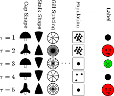
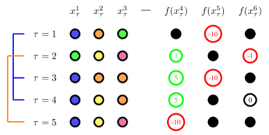
Figure 2: (a) Illustration of the mushroom exploration domain, the rows represent the sequence of mushrooms, with the value of different attributes being displayed on each column. The agent may eat the mushroom to obtain a reward/cost (green/red circle) or choose to ignore it (black circle). (b) Example of a sample sequence of tasks from Section 2.2 with $C\!\!=\!3$, $A\!=\!3$. The left columns indicate the context variables (each color represent a possible value), and the right columns indicate the rewards that have been observed in each task (black when arm has not been pulled). On the left, the true clustering of the tasks (shared mixture component) is displayed. The dictionary of context variables is composed of $D\!=\!5$ different colors in this case.

This problem is conventionally thought of in terms of supervised learning. However, since the agent is allowed to ignore a mushroom, it is actually more akin to a contextual bandit task (?). However in our case, unlike most past work on contextual bandits, early rewards are more valuable than later ones, characterized by a discount factor $\gamma$. This is a critical difference from exploration objectives based on regret that are dominated by the long-term behavior of the agent.

More formally, the mushroom mdp consists of a sequence of mushroom tasks parametrized by $\boldsymbol{x}_{\tau}$ where $\tau=1,2,\dots$. Each parameter vector $\boldsymbol{x}_{\tau}$ contains $C=22$ scalar parameters $x^{1}_{\tau},\dots,x^{C}_{\tau}$ to generate context (the mushroom attributes), and a single scalar parameter $x^{C+1}_{\tau}$ to generate the subtask dynamic (the outcome of eating the mushroom). Denoting $n=C+1$, we have $\boldsymbol{x}_{\tau}=(x^{1}_{\tau},x^{2}_{\tau},\dots,x^{n}_{\tau})$. The mdp dynamics $\operatorname{\mathcal{P}}$ can be described as follows. Let $S$ be the set of states, each of the form $s=(\tau,x^{1}_{\tau},\dots,x^{C}_{\tau},o_{\tau})$, where $o_{\tau}=\Box$ (meaning unobserved) if the mushroom was not eaten in task $\tau$ and $o_{\tau}=x^{C+1}_{\tau}$ otherwise. Choosing the exit action $a_{\text{exit}}$ increments the first state component and updates the context and observation components. Choosing the eat action $a_{\text{eat}}$ updates $o_{\tau}=x^{C+1}_{\tau}$ and delivers a reward/cost.

A simple statistical model

The key aspect of the mushroom task is the joint statistics over the characteristics and danger of the mushrooms. The truth of the matter for the UCI data is actually unclear; it is therefore a stringent test of a planning algorithm whether it is possible to perform at all well based on what can only be a vague, and likely inaccurate model. To do its best, the agent assumes a general non-parametric model that allows for substantial underlying complexity in the true model, but adapts its ongoing characterization as a function of the evidence in the data that has so far been observed (?). We employ one particularly popular non-parametric model called the Chinese Restaurant Process (?) or Dirichlet Process mixture, which postulates that the mushrooms come in a possibly infinite number of mixture components.

The generative model of the mushroom statistics is formally described as follows:

$$\alpha \sim\text{Gamma}(a,b),z_{\tau}\sim\text{CRP}(\alpha),\ \forall\tau\in\mathbb{Z}^{+},$$

$$\boldsymbol{\theta}^{i}_{k} \sim\text{Dirichlet}(\frac{\beta}{D_{i}}),\ \forall i\in\{1,\dots,n\},\forall k\in\mathbb{Z}^{+},$$

$$x^{i}_{\tau} \sim\text{Categorical}(\boldsymbol{\theta}^{i}_{z_{\tau}})\ \forall i\in\{1,\dots,n\},\forall\tau\in\mathbb{Z}^{+},$$

where $\alpha$ is the concentration parameter of the CRP, the $z$ random variables are the cluster assignments. The base measure of this Dirichlet process is assumed to be a symmetric Dirichlet prior with hyperparameter $\beta=1$ ($D_{i}$ is the dimension of $\boldsymbol{\theta}^{i}$, the number of possible observations for $x^{i}$), which together with the conjugate observation model, allows for relatively straightforward inference schemes (see Section S3 for details). The collection $\{\boldsymbol{\theta}^{i}_{k}|i\in\{1,\dots,n\}\}$ of vectors contains the parameters corresponding to each mixture component $k$, the task parameters $\boldsymbol{x}_{\tau}$ for a particular $\tau$ are drawn by first choosing a mixture component $z_{\tau}$ according to the CRP and then using the corresponding $\boldsymbol{\theta}_{z_{\tau}}$ parameters to sample each component of $\boldsymbol{x}_{\tau}$. The infinite-state, infinite-horizon mdp is derived from this generative process by sampling an infinite sequence of tasks ($\tau\rightarrow\infty$) and patching them together.

The data at time $\operatorname{\mathcal{D}}_{t}$ consist of all mushroom attributes and labels observed (the sufficient statistics of the history of transitions), including the current mushroom subtask (and any initial ’free’ examples). The posterior distribution over the dynamics $P(\operatorname{\mathcal{P}}|\operatorname{\mathcal{D}}_{t})$ is then obtained straightforwardly from the posterior over all past and future $\boldsymbol{x}_{\tau}$ (denoted $\boldsymbol{x}_{1:\infty}$), $P(x_{1:\infty}|\operatorname{\mathcal{D}}_{t})$, since $\operatorname{\mathcal{P}}$ is uniquely characterized by $\boldsymbol{x}_{1:\infty}$.

For the mushroom data, we set $D_{i}=12$ for each context dimension $i$ — the maximum number of values for any of the 22 attribute dimensions in the data. This implies $2\cdot 12^{22}\geq 10^{24}$ possible configurations of mushrooms assumed by the model. Since $\alpha$ is not known, we set a generic hyperprior on $\alpha\sim\text{Gamma}(.5,.5)$.

Results in the mushroom task

We stress that the mushroom data were not really generated by the process assumed in the previous section – this is what makes the task somewhat more realistic. Indeed, when the agent lacks prior data, maximizing the return is highly challenging. Randomly eating mushrooms to sample the dataset is a particularly bad strategy because of the cost asymmetry between edible and poisonous mushrooms. A natural point of comparison is the policy of ignoring all mushrooms, which leads to a neutral return of $0$.

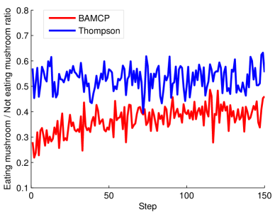
Figure S3: Average rate of exploitation of mushrooms over time for bamcp and ts for the domain described in Section 2.1, when starting with no labelled observations (0 free data condition). For a given step, the reported value is the fraction of time the agent chose to eat the current mushroom (when it had the option to), rather than to skip it.

We ran the Bayes-adaptive agent (bamcp) and ts using this statistical model on the mushroom task. Since the concentration parameter is unknown, it is inferred from data, both influencing, and being influenced by, the exploration. Results are reported in Figure 3a for three different numbers of ’free’ examples. A surprising result is that the Bayes-adaptive agent manages to obtain a positive return when starting with no data, despite the mismatch between true data and generative model. This demonstrates that abstract prior information about structure can guide exploration successfully. Given exactly the same statistical model, ts fails to match this performance; we speculate that this is due to over-optimism, and investigate this further in Section 2.2 and the Supp. material (Fig. S3). When initial data (incl. labels) is provided for free to reduce the prior uncertainty, ts can improve its performance by a large margin but its return remains inferior to a Bayes-adaptive agent in the same conditions.

For the purposes of comparison, we also considered a simpler discriminative statistical model, namely Bayesian Logistic Regression, which (?) suggested for use on contextual bandits. Figure 3 shows the results of applying ts and $\alpha-$UCB (?) in this context. ts does worse with the logistic regression model than with the CRP-based model; this demonstrates the added benefits of a prior that captures many aspects of the data with only a few datapoints. The $\alpha-$UCB algorithm, despite good performance in the long-run on large datasets, is too optimistic to perform well with discounted objectives.

(a)

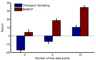
(b)

Figure 3: Exploration-Exploitation results on the mushroom dataset, after 150 steps with $\gamma\!=\!0.97$. (a) Discounted return for bamcp and ts with the CRP model of Section 2.1, including hyperparameter inference. Either starting from scratch from the prior (0 ’free’ data points), or from the prior plus an initial random (labeled) data set of size 5 or 15. At most 75+$\{0,5,15\}$ datapoints can be observed during these 150 steps. (b) Discounted return for ts and $\alpha-$UCB (with $\alpha\!=\!1$ and upper confidence approximation U0 as defined in (?)) when using the Bayesian Logistic Regression model, same task setting as (a). Averaged over 50 runs.

2.2 Non-Parametric Contextual Bandit Sequence model

The mushroom task can be seen as a sequence of subtasks that share structure, but whose order the agent cannot control. Other such domains are adaptive medical treatments where each patient can be understood as the subtask, handling customer interactions, or making decisions to drill for oil at different geological locations. In this section, we consider a generalized version of domains with this characteristic form of shared structure. Further, by addressing environments that were actually drawn from the model, we study planning in the absence of model mis-match.

The key generalization is to allow multiple arms in each subtask (rather than a single eat/exit decision). Using the same notation as Section 2.1, each parameter vector $\boldsymbol{x}_{\tau}$ now contains $C$ scalar parameters $x^{1}_{\tau},\dots,x^{C}_{\tau}$ to generate context, and $Y$ scalar parameters $x^{C+1}_{\tau},\dots,x^{C+Y}_{\tau}$ to generate the actual task dynamics (i.e., denoting $n\!=\!C\!+\!Y$, we have $\boldsymbol{x}_{\tau}=(x^{1}_{\tau},x^{2}_{\tau},\dots,x^{n}_{\tau})$). The generative model is identical otherwise, but now the choices of the agent in any particular task $\tau$ are to either: 1) leave the subtask for the next; or 2) pull any of the $Y$ arms that has not been previously pulled. The mdp states are now of the form $s=(\tau,x^{1}_{\tau},\dots,x^{C}_{\tau},o^{1}_{\tau},\dots,o^{Y}_{\tau})$, where $o^{a}_{\tau}\!=\!\Box$ if arm $a$ has not been pulled in task $\tau$ and $o^{a}_{\tau}\!=\!x^{C+a}_{\tau}$ otherwise. Figure 2b shows the first part of a draw of the generative process including an hypothetical agent trajectory.

The exact setting for the experiments is as portrayed in Figure 2b: with $C=3$ context cues, $A=3$ arms in each task, and $D=5$ possible values of $x$ (i.e., the dimension $D_{i}=5$ for each $\boldsymbol{\theta}$). The function $f$ (that maps values of $x^{a}$ to rewards) is 1-1 with the domain: $\{5,2,0,-1,-10\}$. We drew mdps with different values of the concentration parameter $\alpha\in\{0.1,0.5,1,2,5,10\}$. The agent was assumed to know the generative structure of the mdp; but we considered both cases when it knew the true value of $\alpha$ or just had a generic hyperprior on $\alpha\sim\text{Gamma}(.5,.5)$, and had to learn.

This can be seen as a contextual bandit task (?) with shared structure modeled by a CRP. The difference from the usual definition of contextual bandit is that here, one of the arms has a known reward of $0$ (the exit action) and that we give the option of playing multiple arms for the same context (subtask). In addition, unlike our algorithm, existing work on contextual bandit rarely exploits the unsupervised learning that the context affords even when no label is obtained. Many extensions are possible, including more complex intra-task dynamics (we explore this avenue in the supplementary, Section S4) and more general forms of shared structure; however we focus here on planning rather than modeling.

Results on synthetic data

We investigate the behaviour and performance of Bayesian agents acting in tasks sampled from the non-parametric model above. The reward mapping implies that $E[f(x^{a})]\!=\!-0.8\!<\!0$ for all arms $a$ and for all $\tau$, since all values of $x^{a}$ are equally likely a priori. Thus, again, the strategy $\pi^{\text{exit}}$ of always exiting subtasks (without pulling any arms) is a fair comparison, with value $0$ – a myopic planner based on the posterior mean only should never explore an arm, gaining this value of $0$. Any useful adaptive strategy should be able to obtain a mean return of at least $0$.

We concentrate on two metrics computed during the first $120$ steps of the agent in the environment: the discounted sum of rewards (the formal target for optimization; Figure 4a), and the number of times the agent decides to skip a subtask before trying any of its arms (Figure 4b). The second metric relates to the safe exploration aspect of this task; sometimes optimism is unwarranted because it is more likely to lead to negative outcomes, even when taking into account the long-term consequences of the potential information gain.

(a)

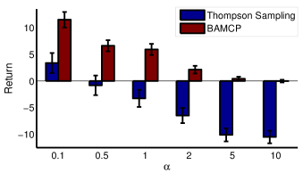
(b)

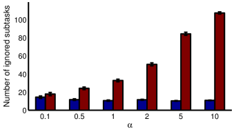
Figure 4: The performance of bamcp and Thompson sampling on the non-parametric bandit task ($\gamma=0.96$) in terms of discounted return (a). The concentration parameter $\alpha$ is known to the algorithm and varies on the x-axis. In (b), the average number of subtasks ignored by each algorithm in the different environmental conditions. Each plotted value is averaged over 200 runs of 120 steps (with 60K forward simulations per step).

We ran bamcp and ts on the task. Figure 4 shows the performance as a function of $\alpha$, when this concentration parameter is known. When the concentration parameter $\alpha$ is small, there will only be a few different mixture components, making for an easy case with little uncertainty about the identity of the mixture components after a few observations, and therefore little uncertainty about the outcome of an arm pull. In the limit of $\alpha\rightarrow 0$, only one cluster will exist and the domain essentially degenerates to a form of multinomial multi-armed bandit problem. As $\alpha$ grows, the identity of a given task’s cluster becomes more uncertain and aliasing grows, so safe exploration becomes more challenging. Learning is slower in that regime too, simply because there are more parameter values to acquire. As $\alpha\rightarrow\infty$, every cluster will be different; this would prevent any kind of generalization and the Bayes-optimal policy will be to skip every subtask $\tau$ (since the a priori expected values of the arms in any given subtask is negative).

Figure 4 shows that bamcp adapts its exploration-exploitation strategy according to the structure in the environment; small values of $\alpha$ justify the risk of exploring and incurring costs but this optimism progressively disappears as $\alpha$ gets larger. This translates into positive return when generalization is feasible, despite the marginal negative expected cost for each arm, and a return close to $0$ when costs cannot be avoided. On the other hand, ts suffers from over-optimism across the board, leading to poor discounted returns, especially when the number of mixture components is large. Intuition for ts’s poor performance comes from considering an extreme case in which all or most subtasks are sampled from a different cluster. Here, past experience provides little information about the value of the arms for the current cluster; thus, discovering these values (which, on average, is expensive) is not likely to help in the future. However, ts samples a single configuration of the arm, mostly informed by the prior in this situation, which likely results in at least one of the arms as having a positive outcome (for the prior, we repeat 3 times a draw having $\frac{2}{5}$ probability of success, so $p=0.784$). ts then, incorrectly, picks this putatively positive arm rather than exiting. Other myopic sample-based exploration strategies, such as Bayesian DP (?) or BOSS (?), would suffer from similar forms of unwarranted optimism — since they also rely on sampling one or more posterior samples according to which they act greedily (see Examples 3-4).

A yet more challenging scenario arises when $\alpha$ is not known to the agent. A Bayesian agent starts with a uninformative (hyper-)prior on $\alpha$ in order to infer the value from data, it also takes into account during planning how its belief about this hyperparameter changes over time. In Figure 5, we observe that the Bayes-adaptive agent is more conservative and explores more safely when $\alpha$ is unknown. As expected, this results in lower returns (compared to when $\alpha$ is known). However, robustness to increased uncertainty is shown by the modest difference.

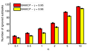
Figure S4: In the domain described in Section 2.2, the average number of ignored subtasks over 120 steps when using bamcp with either $\gamma=0.95$ or $\gamma=0.96$ (Known $\alpha$ scenario). We see that a larger $\gamma$ induces more exploration and risk-taking (fewer subtasks are ignored), showing the sensitivity of Bayes-Adaptive planning to the horizon.

In the suppl. material (Fig. S4), we also show that bamcp is sensitive to the discount factor, highlighting the dependence of the exploration-exploitation strategy to the horizon.

(a)

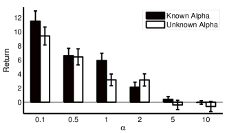
(b)

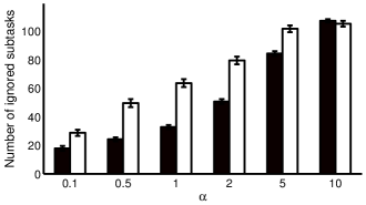
Figure 5: Performance of bamcp for various values of the concentration parameter $\alpha$, with and without hyperparameter inference. The learned Bayes-adaptive policy avoids more subtasks (b) but manages to maintain a similar level of performance (a) despite the uncertainty over $\alpha$. Averaged over 200 runs with 60K simulations for each time-step. The discount parameter is $\gamma=0.96$.

3 Related Work

Many researchers have considered powerful statistical models in the context of sequential decision-making (?; ?), including in exploration-exploitation settings (?; ?). Non-parametric models have been considered in the context of control before (?; ?) but with an emphasis on modeling the data rather than planning. In (?), the authors consider factored mdps whose transitions are modeled using Bayesian Networks. They demonstrate the advantages of having an appropriate prior to capture the existing structure in the true dynamics, at least in a case in which the problems of safe exploration do not arise. For planning, they propose an online Monte-Carlo algorithm with an approximate sampling scheme, however the forward-search is conducted with a depth of 2 and a small branching factor, presumably limiting the benefits of Bayes-adaptivity.

(?) consider a particular form of safe exploration to deal with non-ergodic mdps, but they do not address discounted objectives or structured models.

(?) consider an infinite mdp, combining Bayes-adaptive planning with approximate inference over possible mdps. However the class of models is quite specific to the particular domain they consider. In (?), an hierarchical Dirichlet Process is used to allow for an unbounded number of states in a pomdp and infer the size of the state space from data, this is referred as the ipomdp model. This model is used in a online forward-search planning scheme, albeit of rather limited depth and tested on modestly-sized problems.

In (?), Gaussian Processes (GPs) are employed to infer models of the dynamics from limited data, with excellent empirical performance. However, the uncertainty that the GP captures was not explicitly used for exploration-exploitation-sensitive planning. This is addressed in (?), but with heuristic planning based on uncertainty reduction.

More generally, our task is reminiscent of the case of active classification (?). But while active learning ultimately aims to find an accurate classifier on a labeling budget, we are concerned with a completely different metric, namely discounted return. In particular, a perfectly fine solution in our setting might be to avoid labeling a large part of the input space.

4 Discussion

Model-based Bayesian RL has often been viewed as attractive yet hopeless, particularly in high-dimensional and noisy domains. It had previously been shown that bamcp, an efficient combination of extensions to Monte-Carlo tree search for Bayes-adaptive planning, was computationally viable, and yet very powerful. We showed that alternative, over-optimistic, myopic planning methods such as Thompson Sampling can run into severe problems that bamcp avoids through explicit lookahead computations.

In an attempt to scale Bayes-adaptive planning to real domains, we proposed a contextual-bandit benchmark domain derived from the UCI mushroom dataset and an associated Bayesian non-parametric model for it. In this challenging exploration-exploitation domain, we demonstrated the feasibility and advantages of using a Bayes-Adaptive, or fully Bayesian, agent.

There are various ways to improve planning. Along with generic ideas such as adaptive adjustments of the roll-out policy which exerts a strong influence over the performance of bamcp, it would be interesting to think about more radical departures, such as function approximation within the search tree based on histories and possible future histories.

A remaining open problem is to understand which classes of domains will truly benefit from the computations of Bayes-Adaptive planning (such as the ones explored in this paper), and which will be served just right with a simpler exploration-exploitation approach. Indeed, one can come up with examples where additional computation barely matters, in that the gains are vanishingly small (e.g., the Gittins indices for a multi-armed bandit problem with $\gamma\approx 1$ are hard to obtain, but many myopic policies would do well in that scenario).

We have focused on planning; this means that the challenge now opened up by the success of bamcp is modeling. The non-parametric model of shared structure amongst sub-tasks is readily generalizable to many domains, including ones in which the equivalent of the arms are themselves mdps (see Section S4). A more radical extension would be to something closer to an Indian buffet process (?), in which the whole collection of subtasks also share a measure of structure; this should lead to solutions with collaboration among a set of expert solvers.

Supplementary Material

S1 Bayes-Adaptive Planning

We describe the generic Bayesian formulation of optimal decision-making in an unknown Markov Decision Process (mdp), we refer the reader to (?) and (?) for additional details. An mdp is described as a 5-tuple $M=\langle S,A,\mathcal{P},\mathcal{R},\gamma\rangle$, where $S$ is the set of states, $A$ is the set of actions, $\mathcal{P}:S\times A\times S\rightarrow\mathbb{R}$ is the state transition probability kernel, $\mathcal{R}:S\times A\rightarrow\mathbb{R}$ is a bounded reward function, and $\gamma$ is the discount factor (?). When all the components of the mdp tuple are known, standard mdp planning algorithms can be used to estimate the optimal value function and policy off-line. In general, the dynamics are unknown, and we assume that $\mathcal{P}$ is a latent variable distributed according to a distribution $P(\mathcal{P})$. After observing a history of actions and states $\operatorname{\mathcal{D}}_{t}=s_{1}a_{1}s_{2}a_{2}\dots a_{t-1}s_{t}$ from the mdp, the posterior belief on $\mathcal{P}$ is updated using Bayes’ rule $P(\mathcal{P}|\operatorname{\mathcal{D}}_{t})\propto P(\operatorname{\mathcal{D}}_{t}|\mathcal{P})P(\mathcal{P})$. The uncertainty about the dynamics of the model can be transformed into uncertainty about the current state inside an augmented state space $S^{+}=\mathbfcal{D}$, where $\mathbfcal{D}$ is the set of possible histories. The dynamics associated with this augmented state space are described by

$$\mathcal{P}^{+}(\operatorname{\mathcal{D}},a,\operatorname{\mathcal{D}}as^{\prime}) =\int_{\mathcal{P}}\mathcal{P}(s,a,s^{\prime})P(\mathcal{P}|\operatorname{\mathcal{D}})\,\text{d}\mathcal{P},$$ (1)

$$\mathcal{R}^{+}(\operatorname{\mathcal{D}},a) =R(s,a),$$ (2)

where $s$ is the suffix state of $\operatorname{\mathcal{D}}$. Together, the 5-tuple $M^{+}=\langle S^{+},A,\mathcal{P}^{+},\mathcal{R}^{+},\gamma\rangle$ forms the Bayes-Adaptive mdp (bamdp) for the mdp problem $M$. Since the dynamics of the bamdp are known, it can in principle be solved to obtain the optimal value function associated with each action:

$$Q^{*}(\operatorname{\mathcal{D}}_{t},a)=\max_{\pi}\mathbb{E}_{\pi}\left[\sum_{t^{\prime}=t}^{\infty}\gamma^{t^{\prime}-t}r_{t^{\prime}}|a_{t}=a\right],$$ (3)

where $\pi$ is a policy over the augmented state space, from which the optimal action for each belief-state can be readily derived. Optimal actions in the bamdp are executed greedily in the real mdp $M$ and constitute the best course of action for a Bayesian agent with respect to its prior belief over $\mathcal{P}$. It is obvious that the expected performance of the bamdp policy in the mdp $M$ is bounded above by that of the optimal policy obtained with a fully-observable model, with equality occurring, for example, in the degenerate case in which the prior only has support on the true model.

S2 Examples - Cont.

Example 2

Consider a slight modification of Example 1 where the start state is the second state on the chain, so that with probability $\frac{1}{2}$ the agent is only 1 step away from the reward source (See Figure S1). Clearly, the Bayes-optimal solution is to go left towards the nearest end first. The value of the policy at the start state is $V^{*}=\frac{1}{2}(\gamma+\gamma^{2x+1})$. On the other hand, an algorithm that commits to a particular policy based on a posterior sample will aim for the left or right end of the chain equally often (since they are equally likely). The resulting value of such a strategy is $V=\frac{1}{4}(\gamma+\gamma^{2x-2}(1+\gamma^{3})+\gamma^{4x-1})$, which gives $V=\frac{1}{2}V^{*}$ as $x\rightarrow\infty$.

Figure S1: Illustration of Example 2.

Example 3

Consider a single-step decision between two actions, $a_{1}$ and $a_{2}$, with uncertainty in the payoff as follows. With probability $p$ (case 1), action $a_{1}$ leads to reward $c_{1}<0$ and $a_{2}$ leads to reward $0$. With probability $1-p$ (case 2), action $a_{1}$ leads to reward $1$ and $a_{2}$ leads to negative reward $0$. This is illustrated in Figure S2.

Figure S2: The two possible payoff structures of Example 3.

Conventional ts in this example involves sampling one of the transitions according to the prior and taking the corresponding optimal action. This results in the following expected reward: $V_{TS}=E[r]=p(p\cdot 0+(1-p)\cdot 0)+(1-p)(p\cdot c_{1}+(1-p)\cdot 1)=(1-p)(p\cdot c_{1}+(1-p))$. If $c_{1}$ is arbitrarily large and negative, $V_{TS}$ can be made arbitrarily bad. The Bayes-optimal policy integrates over the possible outcomes, therefore it performs at least as well as always choosing action $a_{2}$ with an expected reward of $0$. This implies $V^{*}\geq 0$. The BOSS algorithm (?) constructs an optimistic mdp based on $K$ posterior samples, so that the best action across all $K$ samples is taken. In this example, it is enough for a single sample of case 2 to be present in these $K$ samples to decide to take action $a_{1}$ (since $r_{2}>r_{1}$), resulting in the following value for BOSS (denoting $X$ to be the number of samples in the set of $K$ samples of case 2): $V_{BOSS}^{ex3}=P(X\geq 1)(p\cdot c_{1}+(1-p))=(1-p^{K})(p\cdot c_{1}+(1-p)):=z(K)$, which is a decreasing function of $K$ (since $c_{1}<0$), showing the cost of this added optimism.

Of course, we usually think of BOSS as being applied to mdps with sequential decisions, but one can readily transform Example 3 in an mdp by putting these 1-step decisions one after the other. We provide details of the construction in Example 4.

Example 4

Consider linking together different instances of Example 3. The agent starts in $s_{0}$, and chooses between $a_{1}$ and $a_{2}$ with payoff described in Example 3. After executing either action, the agent makes a transition to state $s_{1}$, where the process repeats until state $s_{n}$, which itself transits back to $s_{0}$. The outcome of $a_{1}$ and $a_{2}$ (determined by whether $s_{i}$ is of case 1 or 2) is independent across states.

BOSS has a parameter $B$ that decides the number of steps between posterior resampling operations. However, $B$ has no effect in this example for the first $n$ steps. To compute the value of BOSS’s policy from the initial belief state, leveraging the independence assumption, we can employ the value analysis of Example 3 for the first visit of every state. After every state gets visited once, the transition in some states (where action $a_{1}$ was chosen) will be uniquely known and BOSS can perfectly exploit the mdp in these states. For simplicity, we bound the value of the policy by assuming perfect knowledge of the mdp after the first $n$ states: $V_{BOSS}^{ex4}<\sum_{t=0}^{n}\gamma^{t}z(K)+\sum_{t=n+1}^{\infty}\gamma^{t}(1-p)=z(K)\frac{1-\gamma^{n}}{1-\gamma}+\frac{\gamma^{n+1}(1-p)}{1-\gamma}$, where $z(K)=(1-p^{K})(p\cdot c_{1}+(1-p))$ (from Example 3). We can choose $n$ large to make the second term arbitrarily small, whereas the first term again depends on $c_{1}<0$, which we can make arbitrarily bad. Again, the value of the Bayes-optimal policy in this example can easily be lower-bounded as $V^{*}\geq 0$ since the Bayes-optimal policy can at least choose action $a_{2}$ at all times (no exploration).

We stress that PSRL and BOSS do enjoy strong theoretical guarantees for a different objective, namely expected regret; our goal of Bayes adaptivity is a more severe objective because discounting exerts pressure to perform well within a relatively shorter time horizon.

S3 Inference details for the CRP-based contextual-bandit sequence model

• We use a Rao-Blackwellized Gibbs sampler, as described for example in (?). We use the auxiliary variable trick from (?) for tractable inference of the concentration parameter $\alpha$.

• A couple of Gibbs sweeps are performed between every bamcp simulation but this thinning is not necessary for convergence. For Thompson Sampling, we burn in the chain with $500$ Gibbs sweep before selecting the sample used for a particular step.

• Given a setting of the cluster assignments and cluster parameters for the observed subtasks (obtained from the Gibbs sampler), the future subtasks $\boldsymbol{x}_{t:\infty}$ are sampled by running the generative model forward conditioned on the inferred variables.

• In order to improve the planning speed, posterior samples can be memoized at the root of the search tree; the simulations pick from a pool of previously generated samples. The pool gets slowly regenerated.

1 procedure Search( $\operatorname{\mathcal{D}}$ )

2 repeat

3      $\mathcal{P}\sim P(\mathcal{P}|\operatorname{\mathcal{D}})$

4      Simulate($\operatorname{\mathcal{D}},\mathcal{P},0$)

5      until Timeout()

6     return $\displaystyle\operatornamewithlimits{argmax}_{a}\;Q(\operatorname{\mathcal{D}},a)$

7      end procedure

8     

9      procedure Rollout(​ $\operatorname{\mathcal{D}},\mathcal{P},d$ )

10      if $\gamma^{d}Rmax<\epsilon$ then

11           return $0$

12          

13           end $s\leftarrow$ last state in $\operatorname{\mathcal{D}}$

14           $a\sim\pi_{ro}(\operatorname{\mathcal{D}},\cdot)$

15           $s^{\prime}\sim\mathcal{P}(s,a,\cdot)$

16           $r\leftarrow\mathcal{R}(s,a)$

17           return $r\!+\!\gamma$Rollout( $\operatorname{\mathcal{D}}\!as^{\prime},\mathcal{P},d\!+\!1$)

18           end procedure

19          

20           procedure Simulate( $\operatorname{\mathcal{D}},\mathcal{P},d$)

21           if $\gamma^{d}Rmax<\epsilon$ then return $0$

22           $s\leftarrow$ last state in $\operatorname{\mathcal{D}}$

23           if $N(\operatorname{\mathcal{D}})=0$ then

24                for all $a\in A$ do

25                     $N(\operatorname{\mathcal{D}},a)\leftarrow 0$, $Q(\operatorname{\mathcal{D}},a)\leftarrow 0$

26                    

27                     end $a\sim\pi_{ro}(\operatorname{\mathcal{D}},\cdot)$

28                     $s^{\prime}\sim\mathcal{P}(s,a,\cdot)$

29                     $r\leftarrow\mathcal{R}(s,a)$

30                     $R\leftarrow r+\gamma$ Rollout( $\operatorname{\mathcal{D}}\!as^{\prime},\mathcal{P},d$)

31                     $N(\operatorname{\mathcal{D}})\leftarrow 1$, $N(\operatorname{\mathcal{D}},a)\leftarrow 1$

32                     $Q(\operatorname{\mathcal{D}},a)\leftarrow R$

33                     return $R$

34                    

35                     end $a\leftarrow\displaystyle\operatornamewithlimits{argmax}_{b}Q(\operatorname{\mathcal{D}},b)+c\sqrt{\tfrac{\log(N(\operatorname{\mathcal{D}}))}{N(\operatorname{\mathcal{D}},b)}}$

36                     $s^{\prime}\sim\mathcal{P}(s,a,\cdot)$

37                     $r\leftarrow\mathcal{R}(s,a)$

38                     $R\leftarrow r+\gamma$ Simulate($\operatorname{\mathcal{D}}\!as^{\prime},\mathcal{P},d\!+\!1$)

39                     $N(\operatorname{\mathcal{D}})\leftarrow N(\operatorname{\mathcal{D}})+1$

40                     $N(\operatorname{\mathcal{D}},a)\leftarrow N(\operatorname{\mathcal{D}},a)+1$

41                     $Q(\operatorname{\mathcal{D}},a)\leftarrow Q(\operatorname{\mathcal{D}},a)+\frac{R-Q(\operatorname{\mathcal{D}},a)}{N(\operatorname{\mathcal{D}},a)}$

42                     return $R$

43                     end procedure

Algorithm 1 bamcp

1

2procedure GetAction( $\operatorname{\mathcal{D}}$ )

3 $\mathcal{P}\sim P(\mathcal{P}|\operatorname{\mathcal{D}})$

4 $\pi^{*}\leftarrow$ SolveMDP($\mathcal{P},\mathcal{R},\gamma$)

5 $s\leftarrow$ last state in $\operatorname{\mathcal{D}}$ (current state)

6 return $\pi^{*}(s)$

7 end procedure

Algorithm 2 Thompson Sampling

S4 CRP mixture of mdps

To illustrate that our methodology is not restricted to tasks resembling contextual bandits, we consider an extension of the problem in Section 2.2 in which each subtask $\tau$ is a random mdp of a particular class, with contextual information being informative about the class.

This extension is loosely motivated by the following oil exploration problem. Possible drilling sites are considered in a sequence; each site comes with some particular known contextual information (e.g., geological features). One can ignore a drilling site (action $a_{\textit{exit}}$), or (buy acreage and) run one of two types of terrain preparation strategies (actions $a_{0}$ and $a_{1}$ in state $s_{0}$). The outcomes of these two strategies is the potential for either natural gas (state $s_{1}$) or crude oil (state $s_{2}$). Finally, one has to make a final choice about how to exploit (e.g., the type of extraction process, either $a_{2}$ or $a_{3}$), which results in a stochastic payoff for this drilling site: either dry hole with many expenses ($r=-1.5$) or a profitable exploitation ($r=1$).

Figure S5: The extension of the CRP mixture model to mdps, modelling an intermediate decision within each subtask before getting a payoff.

We model this task as in Section 2.2 (each drilling site corresponds to a cluster/subtask $\tau$), except that additional $x_{\tau}$ variables are necessary to establish the transitions between states, in addition to the variables already modeling context and rewards (for states $s_{1}$ and $s_{2}$). The payoff $r_{1,3}$ from executing action $a_{3}$ in $s_{1}$ in subtask $\tau$ is determined by the binary variable $x_{\tau}^{1,3}$ as $r_{1,3}=f(x_{\tau}^{1,3})$ ($f(0)=-1.5,f(1)=1$). In the generative model, $x_{\tau}^{1,3}$ (and other $x_{\tau}^{i,j}$) is determined like the other $x_{\tau}$ variables in Section 2.2. The model is illustrated in Figure S5. The performance of bamcp and ts on simulated data resemble that in the contextual bandits of Section 2.2. bamcp adaptively ignores, explores, or exploits drilling sites depending on the environmental statistics. As in the other examples, with the same statistical model, ts acts too optimistically to do well in terms of discounted return and is less inclined to ignore subtasks. Figure S6-a shows that bamcp is also more conservative when acting within each mdp when $\alpha$ is large, compared to ts. The dynamics of the cumulative return as a function of the steps is presented in Figure S6-b.

(a)

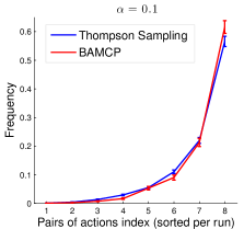
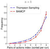
(b)

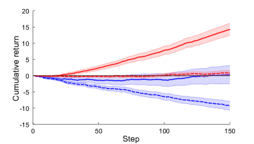
Figure S6: (a) Intratask exploration-exploitation statistics for bamcp and ts in the drilling problem. The distribution of action pairs (sorted in each run) executed inside the mdp subtasks that were explored by the agent. Mean over 100 runs. (b) Comparison of the cumulative return at a fonction of the time step for bamcp (red) and ts (blue). Solid lines: $\alpha=0.1$, dotted line: $\alpha=5$.

References

- [Agrawal and Goyal 2011] Agrawal, S., and Goyal, N. 2011. Analysis of thompson sampling for the multi-armed bandit problem. Arxiv preprint arXiv:1111.1797.
- [Asmuth and Littman 2011] Asmuth, J., and Littman, M. 2011. Approaching Bayes-optimality using Monte-Carlo tree search. In UAI.
- [Asmuth et al. 2009] Asmuth, J.; Li, L.; Littman, M.; Nouri, A.; and Wingate, D. 2009. A Bayesian sampling approach to exploration in reinforcement learning. In UAI.
- [Bache and Lichman 2013] Bache, K., and Lichman, M. 2013. UCI machine learning repository, mushroom dataset. http://archive.ics.uci.edu/ml/datasets/Mushroom.
- [Balcan, Beygelzimer, and Langford 2009] Balcan, M.-F.; Beygelzimer, A.; and Langford, J. 2009. Agnostic active learning. Journal of Computer and System Sciences 75(1):78–89.
- [Chapelle and Li 2011] Chapelle, O., and Li, L. 2011. An empirical evaluation of Thompson sampling. NIPS.
- [Deisenroth and Rasmussen 2011] Deisenroth, M., and Rasmussen, C. 2011. PILCO: A model-based and data-efficient approach to policy search. In ICML.
- [Doshi-Velez et al. 2010] Doshi-Velez, F.; Wingate, D.; Roy, N.; and Tenenbaum, J. 2010. Nonparametric bayesian policy priors for reinforcement learning. NIPS.
- [Doshi-Velez 2009] Doshi-Velez, F. 2009. The infinite partially observable Markov Decision Process. NIPS 22.
- [Duff 2002] Duff, M. 2002. Optimal Learning: Computational Procedures For Bayes-Adaptive Markov Decision Processes. Ph.D. Dissertation, University of Massachusetts Amherst.
- [Escobar and West 1995] Escobar, M. D., and West, M. 1995. Bayesian density estimation and inference using mixtures. Journal of the american statistical association 90(430):577–588.
- [Gittins, Weber, and Glazebrook 1989] Gittins, J.; Weber, R.; and Glazebrook, K. 1989. Multi-armed bandit allocation indices. Wiley Online Library.
- [Griffiths and Ghahramani 2011] Griffiths, T., and Ghahramani, Z. 2011. The Indian buffet process: An introduction and review. JMLR.
- [Guez, Silver, and Dayan 2012] Guez, A.; Silver, D.; and Dayan, P. 2012. Efficient Bayes-Adaptive reinforcement learning using sample-based search. In NIPS.
- [Guez, Silver, and Dayan 2013] Guez, A.; Silver, D.; and Dayan, P. 2013. Scalable and efficient Bayes-adaptive reinforcement learning based on Monte-Carlo tree search. Journal of Artificial Intelligence Research 48:841–883.
- [Jung and Stone 2010] Jung, T., and Stone, P. 2010. Gaussian processes for sample efficient reinforcement learning with rmax-like exploration. In Machine Learning and Knowledge Discovery in Databases. Springer.
- [Kocsis and Szepesvári 2006] Kocsis, L., and Szepesvári, C. 2006. Bandit based Monte-Carlo planning. ECML.
- [Langford and Zhang 2007] Langford, J., and Zhang, T. 2007. The epoch-greedy algorithm for contextual multi-armed bandits. NIPS.
- [Lazaric and Ghavamzadeh 2010] Lazaric, A., and Ghavamzadeh, M. 2010. Bayesian multi-task reinforcement learning. ICML.
- [Li et al. 2012] Li, L.; Chu, W.; Langford, J.; Moon, T.; and Wang, X. 2012. An unbiased offline evaluation of contextual bandit algorithms with generalized linear models. In JMLR Workshop Proc.
- [Martin 1967] Martin, J. 1967. Bayesian decision problems and Markov chains. Wiley.
- [Moldovan and Abbeel 2012] Moldovan, T., and Abbeel, P. 2012. Safe exploration in Markov Decision Processes. In ICML.
- [Moon 1973] Moon, J. 1973. Random walks on random trees. Journal of the Australian Mathematical Society.
- [Orbanz and Teh 2010] Orbanz, P., and Teh, Y. W. 2010. Bayesian nonparametric models. In Encyclopedia of Machine Learning. Springer.
- [Osband, Russo, and Van Roy 2013] Osband, I.; Russo, D.; and Van Roy, B. 2013. (more) efficient reinforcement learning via posterior sampling. In NIPS.
- [Ross and Pineau 2008] Ross, S., and Pineau, J. 2008. Model-based Bayesian reinforcement learning in large structured domains. In UAI.
- [Silver and Veness 2010] Silver, D., and Veness, J. 2010. Monte-Carlo planning in large POMDPs. Advances in Neural Information Processing Systems (NIPS) 2164–2172.
- [Strens 2000] Strens, M. 2000. A Bayesian framework for reinforcement learning. In ICML.
- [Sudderth 2006] Sudderth, E. B. 2006. Graphical models for visual object recognition and tracking. Ph.D. Dissertation, Massachusetts Institute of Technology.
- [Szepesvári 2010] Szepesvári, C. 2010. Algorithms for reinforcement learning. Morgan & Claypool Publishers.
- [Teh 2010] Teh, Y. W. 2010. Dirichlet processes. In Encyclopedia of Machine Learning. Springer.
- [Thompson 1933] Thompson, W. 1933. On the likelihood that one unknown probability exceeds another in view of the evidence of two samples. Biometrika 25(3/4):285–294.
- [Wang et al. 2005] Wang, T.; Lizotte, D.; Bowling, M.; and Schuurmans, D. 2005. Bayesian sparse sampling for on-line reward optimization. In ICML.
- [Wingate et al. 2011] Wingate, D.; Goodman, N.; Roy, D.; Kaelbling, L.; and Tenenbaum, J. 2011. Bayesian policy search with policy priors. In IJCAI.