Abstract

In this paper, instability at an interface between two miscible liquids with identical mechanical properties but different electrical conductivities is analyzed in the presence of an electric field that is perpendicular to the interface. A parallel electric field case was considered in a previous work [1]. A sharp Eulerian interface is considered between the two miscible liquids. Linear stability analysis leads to an analytic solution for the critical condition of instability. The mechanism of instability is analyzed. Key differences between the perpendicular and parallel electric field cases are discussed. The effect of a microchannel geometry is studied and the relevant non-dimensional parameters are identified.

1 Introduction

Instabilities at an interface between two miscible liquids with identical mechanical properties but different electrical conductivities, in the presence of externally applied electric fields, have been studied by Santiago and co-workers [2, 3, 4, 5, 6, 7, 8]. These are instabilities in strong electrolytes and have been termed electrokinetic instabilities. Instabilities with leaky dielectrics have also been considered in literature [9, 10]. In this paper, electrokinetic instabilities are considered where the applied electric field is perpendicular to the interface between two strong electrolytes. This case is expected to be more unstable compared to the parallel electric field case [5].

In prior analytic work [3, 4, 5, 6, 7, 11, 8], a diffuse interface was considered between the two miscible electrolytes. Following the approach in our earlier work [1], we show that the correct behavior in the perpendicular electric field configuration can be also obtained with a sharp Eulerian interface between the two miscible electrolytes. A diffuse interface is not required. The assumption of a sharp interface leads to an easier analytic problem, which results in a compact non-dimensional parameter that determines the unstable behavior of the system. In the above problem, the unstable behavior is quantitatively influenced by the thickness of the diffuse interface between the two liquids. However, the sharp interface case, which corresponds to an experiment where the electric field is applied before the interface has diffused significantly, is an important limiting case.

Although the approach used in this paper is same as that used by Patankar [1], the difference in orientation of the applied electric field brings out different parametric behavior, e.g., the critical condition for instability. The difference in the parametric dependence cannot be intuitively deduced (especially the dependence on electrical conductivities) and is difficult to obtain simply based on experimental data.

In the following sections, the governing equations will be presented first. Instabilities in two geometric configurations – an infinite domain and a microchannel geometry – will be studied.

2 Infinite domain

2.1 Problem formulation

The interface is an Eulerian surface which is defined with respect to the base state. The electrical conductivity in the base state changes sharply at this Eulerian interface. An external electric field $\mathbf{E}$ is applied in the $y$-direction, which is perpendicular to the interface. Liquid $a$ is above the interface (positive values of $y$), and liquid $b$ is below it (negative values of $y$). In the first configuration considered here, the domain is infinite.

The governing equations for this problem can be summarized as follows [1]:

$$\left.\begin{array}[]{l}\varepsilon\nabla^{2}\phi=-\rho_{b},\\ \nabla\cdot(\sigma\mathbf{E})=0,\\ \frac{\displaystyle D\sigma}{\displaystyle Dt}=D_{\sigma}\nabla^{2}\sigma,\\ \nabla\cdot\mathbf{u}=0,\rho\frac{\displaystyle\partial\mathbf{u}}{\displaystyle\partial t}+\rho(\mathbf{u}\cdot\nabla)\mathbf{u}=-\nabla p+\mu\nabla^{2}\mathbf{u}+\rho_{b}\mathbf{E},\end{array}\right\}$$ (1)

where $\varepsilon$ is the permittivity, $\phi$ is the electric potential, $\rho_{b}$ is the bulk charge density in the liquids, $\sigma$ is the electrical conductivity which is different in liquids a and b, $\mathbf{E}$ is the electrical field, $D_{\sigma}$ is the diffusion coefficient for the electrical conductivity, $\mathbf{u}$ is the velocity field, $\rho$ is the density, $p$ is the dynamic pressure (gravity is balanced by the hydrostatic component), and $\mu$ is the viscosity. Liquids $a$ and $b$ are assumed to be strong electrolytes which implies that the electrical conductivities are high. A binary electrolyte is considered [1].

The jump conditions, at the Eulerian interface defined above, are summarized below [1]

$$\rho_{s}=\|\varepsilon\mathbf{E}\|\cdot\mathbf{n},$$ (2)

$$\|\sigma\mathbf{E}\|\cdot\mathbf{n}=0,$$ (3)

$$\|\sigma\mathbf{u}-D_{\sigma}\nabla\sigma\|\cdot\mathbf{n}=0,$$ (4)

$$\|\mathbf{u}\|\cdot\mathbf{n}=0,$$ (5)

$$\mathbf{n}\cdot\|\mathbf{\tau}-\rho\mathbf{u}\mathbf{u}\|\cdot\mathbf{n}=0,\mbox{and}\hskip 5.69046pt\mathbf{t}\cdot\|\mathbf{\tau}-\rho\mathbf{u}\mathbf{u}\|\cdot\mathbf{n}=0,$$ (6)

where $\displaystyle\mathbf{\tau}=-p\mathbf{I}+\mu(\nabla\mathbf{u}+\nabla\mathbf{u}^{T})+\varepsilon\mathbf{E}\mathbf{E}-\frac{\varepsilon}{2}\mathbf{E}\cdot\mathbf{E}\mathbf{I}$, and $\|\|$ denotes the value of the variables at the interface in liquid a minus the value in liquid b. $\mathbf{n}$ is a unit normal to the interface pointing into liquid a.

Semi-infinite domains are considered here in both liquids $a$ and $b$. The sharp Eulerian interface is located at the center of the domain ($y=0$). The material properties $\rho$, $\mu$, and $\varepsilon$ are assumed to be same and constant in both liquids $a$ and $b$. Only the electrical conductivities are considered to be different in liquids $a$ and $b$. Since the domain is unbounded and symmetric with respect to the $z$-direction, the problem is considered to be two-dimensional in the $x$-$y$ plane. It is assumed that there is no electroosmotic flow in the base state. This assumption is discussed further in the Discussion section. The base solution is given by

$$\left.\begin{array}[]{l}\mathbf{u_{0}}=\mathbf{0},\\ \rho_{b0}=0,\\ \sigma_{0}=\sigma_{0}^{a}\hskip 14.22636pt\mbox{in liquid $a$},\\ \sigma_{0}=\sigma_{0}^{b}\hskip 14.22636pt\mbox{in liquid $b$},\\ \displaystyle\mathbf{E_{0}}^{a}=\frac{I_{0}}{\sigma_{0}^{a}}\mathbf{j},\hskip 28.45274pt\displaystyle\mathbf{E_{0}}^{b}=\frac{I_{0}}{\sigma_{0}^{b}}\mathbf{j},\\ \displaystyle\rho_{s0}=\frac{\varepsilon_{0}I_{0}\Delta\sigma_{0}}{\sigma_{0}^{a}\sigma_{0}^{b}},\\ \displaystyle p_{0}^{a}=\frac{\varepsilon I_{0}^{2}}{2(\sigma_{0}^{a})^{2}},\hskip 28.45274pt\displaystyle p_{0}^{b}=\frac{\varepsilon I_{0}^{2}}{2(\sigma_{0}^{b})^{2}},\\ \end{array}\right\}$$ (7)

where $\rho_{b0}$ is the bulk free charge per unit volume inside the fluid, $\rho_{s0}$ is the charge per unit area at the interface, $\Delta\sigma_{0}=\sigma_{0}^{a}-\sigma_{0}^{b}$, and subscript $0$ denotes the variables in the base state. $I_{0}$ is a constant current in $y$-direction. Perturbations are superimposed on the base solution. The conductivity profile in the base state will diffuse with time. However, an approximation is introduced by assuming that the conductivity profile is “frozen” with a sharp jump at the interface. This is not a fully consistent approximation but it is found to be reasonable when the time scale of the instability is short [5, 3].

After linearization, the governing equations, under the assumption of a “frozen” base state, for the perturbations are

$$\left.\begin{array}[]{l}\nabla\cdot\mathbf{u^{\prime}}=0,\\ \displaystyle\varepsilon\nabla^{2}\phi^{\prime}=-\rho_{b}^{\prime},\\ \displaystyle\sigma_{0}\nabla^{2}\phi^{\prime}-\frac{I_{0}}{\sigma_{0}}\frac{\partial\sigma^{\prime}}{\partial y}=0,\\ \displaystyle\frac{\partial\sigma^{\prime}}{\partial t}=D_{\sigma}\nabla^{2}\sigma^{\prime},\\ \displaystyle\rho\frac{\partial\mathbf{u^{\prime}}}{\partial t}=-\nabla p^{\prime}+\mu\nabla^{2}\mathbf{u^{\prime}}+\rho_{b}^{\prime}\mathbf{E_{0}},\end{array}\right\}$$ (8)

where superscript ^′ denotes perturbations. The dimensional form of the perturbations is given by

$$\left(\begin{array}[]{l}\mathbf{u}^{\prime}\\ p^{\prime}\\ \phi^{\prime}\\ \rho_{b}^{\prime}\\ \sigma^{\prime}\\ \ v_{\mbox{int}}^{\prime}\\ \end{array}\right)\mbox{=}\left(\begin{array}[]{l}\mathbf{u}(y)\\ p(y)\\ \phi(y)\\ \rho_{b}(y)\\ \sigma(y)\\ v_{\mbox{int}}\end{array}\right)e^{-ikx+st},$$ (9)

where $v_{\mbox{int}}$ is the $y$ velocity component at the interface, $k$ (a real number) is the wave number of the perturbation, $s$ (a complex number) is the growth rate, and $\mathbf{u}$, $p$, $\phi$, $\rho_{b}$, and $\sigma$ are the amplitudes of the perturbations. An instability is implied by a positive real part of $s$.

The governing equations are non-dimensionalized by using the following scales

$$Length\rightarrow H,\phi^{\prime}\rightarrow\frac{I_{0}H}{\sigma_{m}},E^{\prime}\rightarrow\frac{I_{0}}{\sigma_{m}},\rho_{b}^{\prime}\rightarrow\frac{\varepsilon I_{0}}{H\sigma_{m}},p^{\prime}\rightarrow\frac{\varepsilon I_{0}^{2}}{\sigma_{m}^{2}}$$

$$\sigma^{\prime}\rightarrow\sigma_{m}(=\frac{(\sigma_{0}^{a}+\sigma_{0}^{b})}{2}),Velocity\rightarrow\frac{H\varepsilon I_{0}^{2}}{\sigma_{m}^{2}\mu},time\rightarrow\frac{\mu\sigma_{m}^{2}}{\varepsilon I_{0}^{2}}.$$ (10)

The length scale is $H$ = 1/$k$. The velocity scale is based on the balance between the viscous and electrical forces in the momentum equation. After non-dimensionalization, the perturbation equations become

$$\left.\begin{array}[]{l}\nabla\cdot\mathbf{u^{\prime}}=0,\\ \nabla^{2}\phi^{\prime}=-\rho_{b}^{\prime},\\ \displaystyle\sigma_{0N}^{2}\nabla^{2}\phi^{\prime}-\frac{\partial\sigma^{\prime}}{\partial y}=0,\\ \displaystyle Pe\frac{\partial{\sigma^{\prime}}}{\partial{t}}=\nabla^{2}\sigma^{\prime},\\ \displaystyle Re\frac{\partial\mathbf{u^{\prime}}}{\partial t}=-\nabla p^{\prime}+\nabla^{2}\mathbf{u^{\prime}}+\frac{\rho_{b}^{\prime}}{\sigma_{ON}}\mathbf{j}.\end{array}\right\}$$ (11)

where same symbols have been retained for the non-dimensional variables. The non-dimensional parameters in the governing equations are

$$\left.\begin{array}[]{r}\displaystyle Re=\frac{\rho\varepsilon I_{0}^{2}}{\mu^{2}\sigma_{m}^{2}k^{2}},\\ \displaystyle Pe=\frac{\varepsilon I_{0}^{2}}{\mu D_{\sigma}\sigma_{m}^{2}k^{2}},\\ \displaystyle\sigma_{0N}=\frac{2\sigma_{0}}{\sigma_{0}^{a}+\sigma_{0}^{b}},\end{array}\right\}$$ (12)

where $Re$ is the Reynold’s number, $Pe$ is the Peclet number which is a ratio of convection and diffusion terms, and $\sigma_{0N}$ is the non-dimensionalized value of $\sigma_{0}$ in each liquid.

In the non-dimensional form of Equation (9), we put $k$ = 1 since the length is non-dimensionalized by 1/$k$, and $s$ will be understood to be non-dimensionalized by the inverse of the time scale. Inserting the non-dimensional form of Equation (9) into Equation (11) and simplifying we get

$$\left.\begin{array}[]{l}\displaystyle(D^{2}-1-Pes)\sigma=0,\\ \displaystyle(D^{2}-1)\phi=\frac{D\sigma}{\sigma_{ON}^{2}},\\ \displaystyle(D^{2}-1-Res)(D^{2}-1)\upsilon=-\frac{D\sigma}{\sigma_{ON}^{3}},\\ u=-iD\upsilon,\\ P=(D^{2}-1-Res){Dv},\end{array}\right\}$$ (13)

where $s$ is the non-dimensional growth rate, $D$ is the derivative with respect to $y$, and $u$, $v$ are the $x$, $y$ components of velocity, respectively. The solution of Equation (13) should approach zero as $y\rightarrow\pm\infty$ in liquids $a$ and $b$, respectively. This gives the following solutions for liquids $a$ and $b$

$$\left.\begin{array}[]{l}\sigma^{a}=A^{a}e^{-\lambda y},\\ \displaystyle\phi^{a}=B^{a}e^{-y}+\frac{D\sigma^{a}}{(\sigma_{0N}^{a})^{2}(Pes)},\\ \displaystyle v^{a}=C^{a}e^{-y}+D^{a}e^{-qy}-\frac{D\sigma^{a}}{(Pes-Res)(Pes)(\sigma_{0N}^{a})^{3}},\\ \end{array}\right\}$$ (14)

$$\left.\begin{array}[]{l}\sigma^{b}=A^{b}e^{\lambda y},\\ \displaystyle\phi^{b}=B^{b}e^{y}+\frac{D\sigma^{b}}{(\sigma_{0N}^{b})^{2}(Pes)},\\ \displaystyle v^{b}=C^{b}e^{y}+D^{b}e^{qy}-\frac{D\sigma^{b}}{(Pes-Res)(Pes)(\sigma_{0N}^{b})^{3}},\\ \end{array}\right\}$$ (15)

where $\lambda$ and $q$ are positive and are given by

$$\left.\begin{array}[]{r}\lambda=\sqrt{1+Pes},\\ q=\sqrt{1+Res}.\end{array}\right\}$$ (16)

Superscripts $a$ or $b$ denote liquids $a$ or $b$, respectively. $A,B,C$ and $D$’s with superscript are constants.

The linearized jump conditions for the electrical conductivity at the interface are given by

$$\left.\begin{array}[]{r}\|\sigma\|=0,\\ \|D\sigma\|=Pev_{\mbox{int}}\Delta\sigma_{ON},\end{array}\right\}$$ (17)

where $\displaystyle v_{\mbox{int}}=v^{a}=v^{b}=\frac{(v^{a}+v^{b})}{2}$ at $y$ = 0 is the amplitude of the non-dimensional perturbation velocity at the interface, and $\displaystyle\Delta\sigma_{ON}=\sigma_{ON}^{a}-\sigma_{ON}^{b}$. The jump conditions in Equation (17) follow by assuming that there is no self-sharpening mechanism that creates discontinuities in the electrical conductivity. This is reasonable, since the diffusive behavior of $\sigma$ is important in this problem [12]. The second jump condition in Equation (17) follows from Equation (4). Using these conditions, we get the solution for $A^{a}$ and $A^{b}$ as

$$A^{a}=A^{b}=-\frac{Pev_{\mbox{int}}\Delta\sigma_{ON}}{2\lambda}.$$ (18)

To solve for $B^{a}$ and $B^{b}$, we use the interface jump conditions for the electric potential:

$$\left.\begin{array}[]{r}\|\phi\|=0,\\ \displaystyle\|\sigma_{ON}D\phi\|+\sigma_{y=0}\frac{\Delta\sigma_{0N}}{{\sigma_{0N}^{a}\sigma_{0N}^{b}}}=0.\end{array}\right\}$$ (19)

The first jump condition in Equation (19) follows by assuming that no double layers are formed at the interface. This is reasonable since the interface is not insulating and it is assumed that the current carrying species can pass from one side of the interface to the other [12]. The second jump condition in Equation (19) follows from Equation (3). Thus, $B^{a}$ and $B^{b}$ are

$$B^{a}=\frac{Pev_{\mbox{int}}\triangle\sigma_{0N}^{2}}{4\sigma_{0N}^{a}\sigma_{0N}^{b}(\lambda^{2}-1)\lambda}-\frac{Pev_{\mbox{int}}\triangle\sigma_{0N}(\sigma_{0N}^{a2}+\sigma_{0N}^{b2})}{4(\lambda^{2}-1)\sigma_{0N}^{a}\sigma_{0N}^{b2}},$$ (20)

$$B^{b}=\frac{Pev_{\mbox{int}}\triangle\sigma_{0N}^{2}}{4\sigma_{0N}^{a}\sigma_{0N}^{b}(\lambda^{2}-1)\lambda}+\frac{Pev_{\mbox{int}}\triangle\sigma_{0N}(\sigma_{0N}^{a2}+\sigma_{0N}^{b2})}{4(\lambda^{2}-1)\sigma_{0N}^{a2}\sigma_{0N}^{b}}.$$ (21)

The linearized jump conditions for the velocity (from Equation 5) and the stress (from Equation 6) at $y$ = 0 give

$$\left.\begin{array}[]{r}\|v\|=0,\\ \|u\|=0,\\ \displaystyle\|-p+2Dv-\frac{D\phi}{\sigma_{0N}}\|=0,\\ \displaystyle\|D^{2}v+v-\frac{\phi}{\sigma_{0N}}\|=0.\end{array}\right\}$$ (22)

Note that the jump condition for $u$ is due to the no-slip condition. This is reasonable since no double-layers are formed at the interface. Inserting the solutions for velocity in Equations (14) and (15) into Equation (22), we get five homogeneous equations for five unknowns: $C^{a}$, $C^{b}$, $D^{a}$, $D^{b}$, and $v_{\mbox{int}}$:

$$\left(\begin{array}[]{ccccc}1&-1&1&-1&f_{1}\\ 1&1&q&q&f_{2}\\ 1&1&q^{3}&q^{3}&f_{3}\\ 1&-1&q&q^{2}&f_{4}\\ 1&1&1&1&f_{5}\\ \end{array}\right)\left(\begin{array}[]{l}C^{a}\\ C^{b}\\ D^{a}\\ D^{b}\\ v_{\mbox{int}}\end{array}\right)\mbox{=}\left(\begin{array}[]{l}0\\ 0\\ 0\\ 0\\ 0\end{array}\right)$$ (23)

$$f_{1} = -\frac{Pe\Sigma(\Gamma-2)}{2(\lambda^{2}-1)(\lambda^{2}-q^{2})}\sqrt{\frac{\Gamma-3}{\Gamma+1}},$$ (24)

$$f_{2} = \frac{\lambda Pe\Sigma\Gamma}{2(\lambda^{2}-1)(\lambda^{2}-q^{2})},$$ (25)

$$f_{3} = \frac{\lambda^{3}Pe\Gamma}{2(\lambda^{2}-1)(\lambda^{2}-q^{2})}+\frac{Pe\Gamma}{2(\lambda^{2}-1)}(\frac{1}{\lambda}+(\Gamma-1)-\lambda\Gamma),$$ (26)

$$f_{4} = \frac{\lambda^{2}Pe\Sigma(\Gamma-2)}{2(\lambda^{2}-1)(\lambda^{2}-q^{2})}\sqrt{\frac{\Gamma+1}{\Gamma-3}}+\frac{Pe\Gamma}{2(\lambda^{2}-1)}\sqrt{\frac{\Gamma-3}{\Gamma+1}}$$ (27)

$$+ \frac{Pe\Sigma(\Gamma-1)^{2}}{2(\lambda^{2}-1)\sqrt{(\Gamma+1)(\Gamma-3)}}-\frac{Pe\Sigma(\Gamma-2)}{2(\lambda^{2}-1)}\sqrt{\frac{\Gamma+1}{\Gamma-3}},$$

$$f_{5} = \frac{Pe\Sigma\Gamma}{2(\lambda^{2}-1)(\lambda^{2}-q^{2})}-2.$$ (28)

where $\displaystyle\Sigma=\frac{\Delta\sigma_{0N}^{2}}{\sigma_{0N}^{a2}\sigma_{0N}^{b2}}$ and $\displaystyle\Gamma=\frac{\sigma_{0N}^{a}}{\sigma_{0N}^{b}}+\frac{\sigma_{0N}^{b}}{\sigma_{0N}^{a}}+1$. The dispersion equation is obtained by setting the determinant of the matrix to zero.

2.2 The critical condition for instability

The dispersion equation obtained from manipulations in Mathematica is

$$-(4\Gamma(1+\sqrt{1+ST})((1+S)^{\frac{3}{2}}\sqrt{1+ST}+$$

$$\sqrt{1+S}(1+ST)+(1+S)\sqrt{1+ST}(1+\sqrt{1+ST})))$$

$$+P_{\Sigma}(\sqrt{1+S}-\Gamma\sqrt{1+S}+\sqrt{1+ST})=0,$$ (29)

where $S=Pes$, $P_{\Sigma}=Pe\Sigma\Gamma$, and $\displaystyle T=\frac{Re}{Pe}$. The maximum growth rate for this problem is the largest root of the dispersion equation. It is verified that the maximum growth rate is positive and real.

When the system is marginally stable i.e. when the maximum growth rate $S=0$, then $P_{\Sigma}$ is found to be independent of $T$ and is a function of $\Gamma$. The marginal stability condition gives the critical condition for the onset of instability. It is given by

$$\left.\begin{array}[]{r}\displaystyle P_{\Sigma}^{cri}=\frac{32\Gamma}{\Gamma-2},\\ \displaystyle\Rightarrow(\frac{\varepsilon{E_{\mbox{mean}}}^{2}}{D_{\sigma}\mu k^{2}})^{cri}=\frac{32}{(\Gamma-2)\Sigma},\end{array}\right\}$$ (30)

where $\displaystyle E_{\mbox{mean}}=\frac{I_{0}}{\sigma_{m}}$. Figure (1) shows a plot of $P_{\Sigma}^{cri}$ as a function of $\Gamma$.

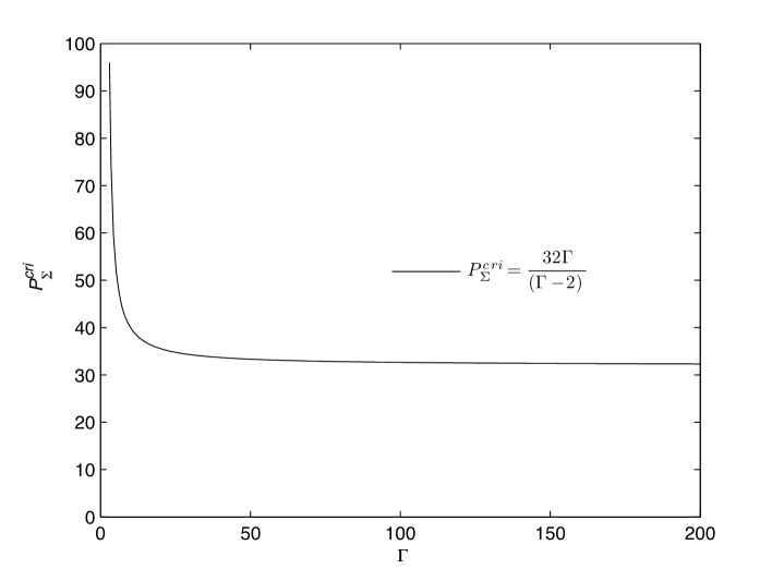
Figure 1: The marginal stability curve ($P_{\Sigma}^{cri}$ vs. $\Gamma$) identifying the critical condition for the onset of instability. The region above the curve indicates unstable conditions.

2.3 The mechanism of instability

An approach similar to that in our earlier work [1] is followed. Streamlines spanning one wavelength are plotted for a typical unstable mode in Figure (2).

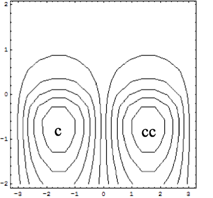
Figure 2: Streamlines of an unstable mode in an infinite domain where the applied electric field is perpendicular to the interface between the two liquids. ’c’ denotes clockwise rotation of the fluid and ’cc’ denotes counterclockwise rotation.

The parameters are $T=0.05$, $S=25$, $P_{\Sigma}=683.3914$, $\displaystyle\frac{\sigma_{0N}^{a}}{\sigma_{0N}^{b}}=10$ , and $\Gamma=11.1$.

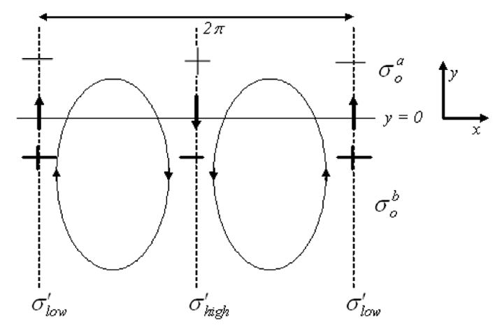
Figure 3: A typical unstable flow cell is depicted. Higher conductivity fluid is in the upper half and the lower conductivity fluid is in the lower half. Interfacial velocity perturbations are shown by bold arrows. Positive and negative signs show the locations of high and low values of the perturbed electrical conductivity. Bold signs indicate that there is greater bulk charge in the lower conductivity fluid.

A perturbation in the interfacial velocity, $v^{\prime}_{\mbox{int}}=cos(x)$, leads to a perturbation in the electrical conductivity due to the electrohydrodynamic coupling in Equation (17), and Equations (14), (15) and (18):

$$\sigma^{\prime a}=-\frac{Pe\Delta\displaystyle{\sigma_{ON}}}{2\lambda}e^{-\lambda y}cos(x),\hskip 28.45274pt\sigma^{\prime b}=-\frac{Pe\Delta\displaystyle{\sigma_{ON}}}{2\lambda}e^{\lambda y}cos(x).$$ (31)

It follows from Equation (31) that a region of lower electrical conductivity is formed when $v_{\mbox{int}}$ is maximum, and higher electrical conductivity is formed when $v_{\mbox{int}}$ is minimum. This is depicted in Figure (3) with vertical bold arrows at locations of maximum and minimum velocities. Perturbations in the electrical conductivity leads to a perturbation in the bulk charge density (Equation 11) according to $\rho_{b}^{\prime}=-\frac{1}{\displaystyle{\sigma_{ON}^{2}}}\displaystyle{\frac{\partial\sigma^{\prime}}{\partial y}}$. Thus, we get

$$\rho_{b}^{\prime a}=-\frac{Pe\Delta\displaystyle{\sigma_{ON}}}{2\displaystyle{\sigma_{ON}^{a2}}}e^{-\lambda y}cos(x),\hskip 28.45274pt\rho_{b}^{\prime b}=\frac{Pe\Delta\displaystyle{\sigma_{ON}}}{2\displaystyle{\sigma_{ON}^{b2}}}e^{\lambda y}cos(x).$$ (32)

This leads to an asymmetric bulk charge distribution in the domain as seen in Figure (3). The consequent electrical body force in the fluid gives rise to a cellular flow that reinforces the initial perturbation in velocity and causes instability.

2.4 Comparison with the parallel electric field case

It has been reported that when an electric field is applied perpendicular to the interface the system is more unstable compared to the parallel electric field case [2].

We consider this issue by comparing the critical condition for instability for these cases. The following critical condition for instability of the parallel electric field case is given in our previous work [1]:

$$\left.\begin{array}[]{r}\displaystyle P_{\Sigma\parallel}^{cri}=32,\\ \displaystyle\Rightarrow(\frac{\varepsilon{E_{0}}^{2}}{D_{\sigma}\mu k^{2}})^{cri}=\frac{32}{\Sigma_{\parallel}},\end{array}\right\}$$ (33)

where $\displaystyle\Sigma_{\parallel}=\frac{\Delta\sigma_{0N}^{2}}{\sigma_{0N}^{a}\sigma_{0N}^{b}}.$ Comparison between Equations (30) and (33) implies that the perpendicular electric field case is more unstable compared to the parallel electric field case. This is discussed below.

Consider parameters: $\sigma^{a}/\sigma^{b}=10$ , $\mu=0.001kg/ms$, $\varepsilon=6.9\times 10^{-10}C/Vm$, $\rho=1000kg/m^{3}$ , and $D_{\sigma}=10^{-9}m^{2}/s$. We express $\Sigma$’s in terms of $\sigma_{a}$ and $\sigma_{b}$ rather than $\sigma_{0N}^{a}$ and $\sigma_{0N}^{b}$ in both parallel and perpendicular electric field cases, Thus

$$\Sigma_{\parallel}=\frac{(\sigma^{a}-\sigma^{b})^{2}}{\sigma^{a}\sigma^{b}}=8.1.$$ (34)

Using equation (33), we get

$$(\frac{\varepsilon{E_{0}}^{2}}{D_{\sigma}\mu k^{2}})^{cri}=\frac{32}{8.1}\approx 3.95.$$ (35)

For the perpendicular electric field case, we have

$$\left.\begin{array}[]{r}\Sigma=\displaystyle{(\frac{(\sigma^{a})^{2}-(\sigma^{b})^{2}}{2\sigma^{a}\sigma^{b}})^{2}}=24.5025,\\ \Gamma=\displaystyle{\frac{\sigma^{a}}{\sigma^{b}}+\frac{\sigma^{b}}{\sigma^{a}}}+1=11.1.\end{array}\right\}$$ (36)

Using equation (30), we get

$$(\frac{\varepsilon{E_{\mbox{mean}}}^{2}}{D_{\sigma}\mu k^{2}})^{cri}=\frac{32}{\Sigma(\Gamma-2)}=\frac{32}{24.5025\times 9.1}\approx 0.143.$$ (37)

Comparing Equations (35) and (37), we see that the electric field needed to achieve the instability in the parallel case is larger than the perpendicular electric field case.

This difference is due to the difference in the flow pattern in the unstable modes. The parallel electric field case has a different cellular flow pattern in the unstable mode (see [1]). Two pairs of counter rotating vortices are produced in the parallel electric field case. This flow pattern is much less asymmetric and gives rise to weaker flows. In the perpendicular electric field case the asymmetry is much stronger primarily due to the current flowing perpendicular to the interface in the base state. This results in stronger destabilizing forces in the perpendicular electric field case thus making it more unstable.

We consider a single parameter above simply for the purpose of comparing parallel and perpendicular electric field cases at typical conditions that are known. Otherwise, the critical conditions for the two cases (parallel and perpendicular) allow comparison over the entire parameter range which shows a similar trend that the perpendicular electric field case is more unstable.

3 Shallow channel

3.1 Problem formulation

Next we apply the linear stability analysis to the case of a shallow microchannel geometry (Figure 4) that is typical in microfluidic devices [2, 5]. The objective is to understand the influence of the device geometry on the instability.

An external electrical field applied perpendicular to the interface ($y$-direction) between two liquids $a$ and $b$ in a domain that is unbounded in the $x$ direction. It is assumed that there is no electroosmotic flow, and there is no charges in the base state. The base state is the same as that in Equation (LABEL:eqn:basesol) and the perturbation equations are given by Equation (8).

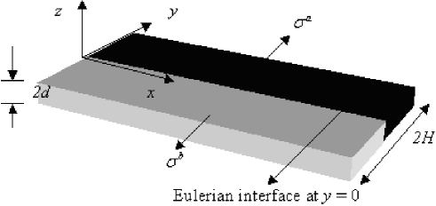
Figure 4: The shallow channel geometry.

The governing equations are non-dimensionalized by using the following scales

$$x,y\rightarrow H,z\rightarrow d,\phi^{\prime}\rightarrow\frac{I_{0}H}{\sigma_{m}},E^{\prime}\rightarrow\frac{I_{0}}{\sigma_{m}},\rho_{b}^{\prime}\rightarrow\frac{\varepsilon I_{0}}{H\sigma_{m}},p^{\prime}\rightarrow\frac{\varepsilon I_{0}^{2}}{\sigma_{m}^{2}},$$

$$\sigma^{\prime}\rightarrow\sigma_{m}(=\frac{(\sigma_{0}^{a}+\sigma_{0}^{b})}{2}),Velocity\rightarrow\frac{H\beta^{2}\varepsilon I_{0}^{2}}{\sigma_{m}^{2}\mu},time\rightarrow\frac{\mu\sigma_{m}^{2}}{\beta^{2}\varepsilon I_{0}^{2}}.$$ (38)

where $\beta=d/H<<1$ for a shallow channel.

For a shallow channel, $\beta\rightarrow 0$ in the governing equations which is the Hele-Shaw limit. This leads to $\phi^{\prime}=\phi^{\prime}(x,y)$, $\sigma^{\prime}=\sigma^{\prime}(x,y)$, and $\rho_{b}^{\prime}=\rho_{b}^{\prime}(x,y)$. It is assumed that $\partial\phi^{\prime}/\partial z=\partial\sigma^{\prime}/\partial z=0$ at the top and bottom walls [1].

In the Hele-Shaw limit the velocity component in the vertical direction is zero, the pressure $p^{\prime}=p^{\prime}(x,y)$, and the horizontal velocity in the $x-y$ plane is of the form $\mathbf{u^{\prime}}(x,y,z)=1.5(1-z^{2})\mathbf{u}_{m}^{\prime}(x,y)$ [5, 8, 1], where the variables are non-dimensional. As discussed earlier [1] $\mathbf{u}_{m}^{\prime}$ is the perturbation velocity at a given location that is averaged with respect to the $z$ direction. The governing equations become [5, 8, 1]

$$\left.\begin{array}[]{l}\nabla_{H}\cdot\mathbf{u}_{m}^{\prime}=0,\\ \nabla_{H}^{2}\phi^{\prime}=-\rho_{b}^{\prime},\\ \displaystyle\sigma_{0N}^{2}\nabla_{H}^{2}\phi^{\prime}-\frac{\partial\sigma^{\prime}}{\partial y}=0,\\ \displaystyle Pe\frac{\partial{\sigma}}{\partial{t}}=\nabla_{H}^{2}\sigma,\\ \displaystyle Re\beta^{2}\frac{\partial\mathbf{u}_{m}^{\prime}}{\partial t}=-\nabla p^{\prime}+\beta^{2}\nabla_{H}^{2}\mathbf{u}_{m}^{\prime}-3\mathbf{u}_{m}^{\prime}+\frac{\rho_{b}^{\prime}}{\sigma_{ON}}\mathbf{j},\end{array}\right\}$$ (39)

where $\nabla_{H}$ denotes the gradient in the $x-y$ plane. All variables carry same meaning as before unless specified otherwise. The non-dimensional parameters in this case are given by

$$\left.\begin{array}[]{r}\displaystyle Re=\frac{\beta^{2}H^{2}\rho\varepsilon I_{0}^{2}}{\mu^{2}\sigma_{m}^{2}},\\ \displaystyle Pe=\frac{\beta^{2}H^{2}\varepsilon I_{0}^{2}}{\mu D_{\sigma}\sigma_{m}^{2}},\\ \displaystyle\sigma_{0N}=\frac{2\sigma_{0}}{\sigma_{0}^{a}+\sigma_{0}^{b}}.\end{array}\right\}$$ (40)

As discussed earlier [1], the terms involving $\beta^{2}$ in the last of equation (39) should be dropped in the Hele-Shaw limit. However, those terms may be retained to approximately capture the viscous effects due to the flow in the $x-y$ plane [5, 8]. Matching of the “inner” solution in the thin viscous layers near the vertical walls with the “outer” Hele-Shaw solution is necessary to obtain a formal solution. Such an analysis will not be considered here. Instead, an approximate approach based on Equation (39) will be considered [5, 8]. This will also facilitate comparison with the parallel electric field case considered earlier [1].

The novelty of our effort is the use of a sharp interface approach in the linear stability analysis. Assuming perturbations of the form given by Equation (9) the governing equations become

$$\left.\begin{array}[]{l}\displaystyle(D^{2}-k^{2}-Pes)\sigma=0,\\ \displaystyle(D^{2}-k^{2})\phi=\frac{D\sigma}{\sigma_{ON}^{2}},\\ \displaystyle(D^{2}-k^{2}-Res-\frac{3}{\beta^{2}})(D^{2}-k^{2})v_{m}-\frac{k^{2}D\sigma}{\beta^{2}\sigma_{ON}^{3}},\\ \displaystyle u_{m}=-\frac{iDv_{m}}{k},\\ \displaystyle p=\frac{(\beta^{2}(D^{2}-k^{2})-\beta^{2}s-3){Dv_{m}}}{k^{2}}.\end{array}\right\}$$ (41)

Solutions of the governing equations are given by

$$\left.\begin{array}[]{l}\sigma^{a}=A^{a}\sinh{\lambda y}+B^{a}\cosh{\lambda y},\\ \displaystyle\phi^{a}=C^{a}\sinh{\lambda y}+D^{a}\cosh{\lambda y}+\frac{D\sigma^{a}}{(\sigma_{0N}^{a})^{2}(\lambda^{2}-k^{2})},\\ \displaystyle v^{a}=E^{a}\sinh{\lambda y}+F^{a}\cosh{\lambda y}+G^{a}\sinh{\lambda y}+H^{a}\cosh{\lambda y}\\ \hskip 28.45274pt-\displaystyle{k^{2}\frac{D\sigma^{a}}{\beta^{2}(\sigma_{0N}^{a})^{3}(\lambda^{2}-q^{2})(\lambda^{2}-k^{2})}},\\ \end{array}\right\}$$

$$\left.\begin{array}[]{l}\sigma^{b}=A^{b}\sinh{\lambda y}+B^{b}\cosh{\lambda y},\\ \displaystyle\phi^{b}=C^{b}\sinh{\lambda y}+D^{b}\cosh{\lambda y}+\frac{D\sigma^{b}}{(\sigma_{0N}^{b})^{2}(\lambda^{2}-k^{2})},\\ \displaystyle v^{b}=E^{b}\sinh{\lambda y}+F^{b}\cosh{\lambda y}+G^{b}\sinh{\lambda y}+H^{b}\cosh{\lambda y}\\ \hskip 28.45274pt\displaystyle{k^{2}\frac{D\sigma^{b}}{\beta^{2}(\sigma_{0N}^{b})^{3}(\lambda^{2}-q^{2})(\lambda^{2}-k^{2})}}.\\ \end{array}\right\}$$

Superscripts $a$ or $b$ denote liquids $a$ or $b$, respectively. $A,B,C,D,E,F,G$ and $H$ are constants. $\lambda$ and $q$ are positive and are given by

$$\left.\begin{array}[]{l}\lambda=\sqrt{k^{2}+Pes},\\ \displaystyle q=\sqrt{k^{2}+Res+\frac{3}{\beta^{2}}}.\end{array}\right\}$$

Now we must use the boundary and interface conditions to solve for the constants in the solution. The linearized jump conditions for electrical conductivity at the interface are

$$\left.\begin{array}[]{l}\|\sigma\|=0,\\ \|D\sigma\|=Pev_{int}\sigma_{0N}.\end{array}\right\}$$

The linearized boundary conditions for electrical conductivity at the side walls (i.e. at $y=\pm 1$) are given by $D\sigma=0$. The interface conditions together with the boundary conditions give the following solution for the constants

$$\left.\begin{array}[]{l}\displaystyle A^{a}=-A^{b}=-\frac{Pev_{\mbox{int}}\Delta\sigma_{0N}}{2\lambda},\\ \displaystyle B^{a}=B^{b}=-\frac{Pev_{\mbox{int}}\Delta\sigma_{0N}}{2\lambda\tanh\lambda},\end{array}\right\}$$

where $\Delta\sigma_{0N}=\sigma_{0N}^{a}-\sigma_{0N}^{b}$, and $\displaystyle v_{\mbox{int}}=v_{m}^{a}=v_{m}^{b}=\frac{v_{m}^{a}+v_{m}^{b}}{2}$ at $y=0$ is the $y$ component of velocity at the interface.

The interface conditions for the electrical potential are

$$\left.\begin{array}[]{l}\|\phi\|=0,\\ \displaystyle\|\sigma_{0N}D\phi\|+\sigma_{y=0}\frac{\Delta\sigma_{0N}}{\sigma_{0N}^{+}\sigma_{0N}^{-}}\end{array}\right\}\mbox{at y=0}.$$

Since there are electrodes at $y=\pm 1$, there is no perturbation of the electric potential at those boundaries. This implies $\phi=0$ at $y=\pm 1$. Using these interface and boundary conditions we solve for $C^{a}$, $C^{b}$, $D^{a}$, and $D^{b}$ to obtain

$$\left.\begin{array}[]{l}\displaystyle{C^{a}=\frac{\Delta\sigma_{0N}}{4\sigma_{0N}^{a}\sigma_{0N}^{b}}\frac{k}{\lambda^{2}-k^{2}}(\frac{-1}{\tanh\lambda})\frac{Pev_{\mbox{int}}\Delta\sigma_{0N}}{\lambda}+\frac{\mbox{Pe}v_{\mbox{int}}\Delta\sigma_{0N}\sigma_{0N}^{b}}{4(\lambda^{2}-k^{2})\tanh k}\frac{\sigma_{0N}^{a2}+\sigma_{0N}^{b2}}{\sigma_{0N}^{a2}\sigma_{0N}^{b2}}},\\ \displaystyle{C^{b}=\frac{\Delta\sigma_{0N}}{4\sigma_{0N}^{a}\sigma_{0N}^{b}}\frac{k}{\lambda^{2}-k^{2}}(\frac{1}{\tanh\lambda})\frac{Pev_{\mbox{int}}\Delta\sigma_{0N}}{\lambda}+\frac{\mbox{Pe}v_{\mbox{int}}\Delta\sigma_{0N}\sigma_{0N}^{a}}{4(\lambda^{2}-k^{2})\tanh k}\frac{\sigma_{0N}^{a2}+\sigma_{0N}^{b2}}{\sigma_{0N}^{a2}\sigma_{0N}^{b2}}},\\ D^{a}=-\tanh{k}C^{a},\\ D^{b}=\tanh{k}C^{b}.\end{array}\right\}$$

The interface conditions for velocity are $\|Dv_{m}\|=0$ (which follows from $\|u_{m}\|=0$) and $\|v_{m}\|=0$ at $y=0$. The velocity boundary conditions are $v_{m}=0$ and $Dv_{m}=0$ (i.e. $u_{m}=0$) at $y=\pm 1$. The stress conditions at the interface are $\displaystyle\|-p+2\beta^{2}Dv-\frac{D\phi}{\sigma_{0N}}\|=0$ and $\displaystyle\|D^{2}v+v-\frac{\phi}{\sigma_{0N}}\|=0$. Using these conditions together with Equations (3.1) and (3.1) we get eight equations for the constants $E$, $F$, $G$ and $H$ in liquids $a$ and $b$. Only four of those equations and the equation $\displaystyle v_{\mbox{int}}=\frac{v_{m}^{a}+v_{m}^{b}}{2}$ give the maximum growth rate:

$$\left(\begin{array}[]{ccccc}\sinh k&\cosh k&\sinh q&\cosh q&0\\ k\cosh k&k\sinh k&q\cosh q&q\sinh q&\displaystyle{-\frac{k^{2}\lambda^{2}P_{\Sigma}}{2\lambda\sinh\lambda(\lambda^{2}-q^{2})(\lambda^{2}-k^{2})}}\\ q&0&q&0&\displaystyle{-\frac{k^{2}\lambda^{2}P_{\Sigma}}{2\lambda\tanh\lambda(\lambda^{2}-q^{2})(\lambda^{2}-k^{2})}}\\ k^{3}&0&q^{3}&0&f(k,\lambda,q,\Gamma,P_{\Sigma})\\ 0&1&0&1&\displaystyle{(\frac{k^{2}P_{\Sigma}}{2(\lambda^{2}-k^{2})(\lambda^{2}-q^{2})-2})}\end{array}\right)\left(\begin{array}[]{l}E^{s}\\ F^{t}\\ G^{s}\\ H^{t}\\ v_{\mbox{int}}\end{array}\right)$$

$$=\left(\begin{array}[]{l}0\\ 0\\ 0\\ 0\\ 0\end{array}\right)$$ (42)

In Equation (42), $E^{s}=E^{a}-E^{b}$ and $F^{t}=F^{a}+F^{b}$. $G^{s}$ and $H^{t}$ are defined similarly. $P_{\Sigma}=Pe\Sigma\Gamma/\beta^{2}$, where $\displaystyle\Sigma=\frac{\Delta\sigma_{0N}^{2}}{\sigma_{0N}^{a2}\sigma_{0N}^{b2}}$ and $\displaystyle\Gamma=\frac{\sigma_{0N}^{a}}{\sigma_{0N}^{b}}+\frac{\sigma_{0N}^{b}}{\sigma_{0N}^{a}}+1$.

The dispersion equation is once again obtained by setting the determinant of the matrix, above, equal to zero.

3.2 Results

The dispersion equation gives $P_{\Sigma}$ as a function of $\lambda,k,q,\mbox{and}\hskip 2.84544pt\Gamma$.

$$P_{\Sigma}=-(32\Gamma\lambda(-k^{2}+\lambda^{2})q(k^{2}-q^{2})(\lambda^{2}-q^{2})(k\mbox{cosh}q\mbox{sinh}k-q\mbox{cosh}k\mbox{sinh}q))$$

$$/(k^{2}(\frac{1}{2}(-1+\Gamma)k\lambda q(\lambda^{2}-q^{2})\mbox{coth}k(31+\mbox{cosh}k^{2}-16\mbox{cosh}k\mbox{cosh}q+\mbox{sinh}k^{2})$$

$$+8\mbox{coth}\lambda(q(-\Gamma\lambda^{2}q^{2}+k^{2}((-2+\Gamma)\lambda^{2}+2q^{2}))-q(-\Gamma\lambda^{2}q^{2}+k^{2}((-2+\Gamma)\lambda^{2}+2q^{2}))$$

$$\mbox{cosh}k\mbox{cosh}q+k(k^{2}((-1+\Gamma)\lambda^{2}+q^{2})+q^{2}((-1+\Gamma)\lambda^{2}+q^{2}))\mbox{sinh}k\mbox{sinh}q)+$$

$$\lambda(-8q\mbox{cosh}q(-(-1+\Gamma)k(\lambda^{2}-q^{2})\mbox{csch}k+\Gamma\lambda(k^{2}-q^{2})\mbox{csch}\lambda+k(\Gamma k^{2}+$$

$$\lambda^{2}-\Gamma\lambda^{2}-q^{2})\mbox{sinh}k+\mbox{cosh}k(8\Gamma\lambda q(k^{2}-q^{2})\mbox{csch}\lambda+(-1+\Gamma)kq(\lambda^{2}-q^{2})\mbox{sinh}k-$$

$$8(q^{2}((-1+\Gamma)\lambda^{2}+q^{2})+k^{2}((-1+\Gamma)\lambda^{2}+(1-2\Gamma)q^{2}))\mbox{sinh}q)))).$$

$P_{\Sigma}$ can also be expressed as a function of $\displaystyle k,\mbox{Pes},(\mbox{Res}+\frac{3}{\beta^{2}}),\mbox{and}\hskip 2.84544pt\Gamma$ i.e.

$$P_{\Sigma}=f(\lambda,k,q,\Gamma)=g(k,\mbox{Pes},(\mbox{Res}+\frac{3}{\beta^{2}}),\Gamma).$$ (44)

For marginal stability at low Re we take $Re\rightarrow 0$ and $s\rightarrow 0$. In this case $P_{\Sigma}$ depends on $\Gamma,k,\mbox{and}\hskip 2.84544pt\beta$ i.e.

$$P_{\Sigma}=f(\Gamma,k,\beta).$$ (45)

The trends of $P_{\Sigma}$ will be considered next. We will use parameters corresponding to typical experimental values [5]: $d=5.5\mu m$, $H=78\mu m$, $\rho=1000kg/m^{3}$, $\mu=0.001kg/ms$, $\varepsilon=6.9\times 10^{-10}C/Vm$, $D_{\sigma}=10^{-9}m^{2}/s$, and $\displaystyle\frac{\sigma_{0}^{a}}{\sigma_{0}^{b}}=10$. This implies $\beta=0.07$, $\Gamma=11.1$, and $\Sigma=24.5$. The only free variables are $I_{0}/\sigma_{m}$ and $k$. In this case, $P_{\Sigma}$ is therefore the non-dimensional parameter that represents the variation of $I_{0}/\sigma_{m}$ which is an average measure of the external electric field.

Figure (5) shows the marginal stability curve of $P_{\Sigma}$ vs.the wavenumber $k$ obtained from the dispersion equation discussed above. It is seen that there is a critical value of the $P_{\Sigma}$ (or correspondingly $I_{0}/\sigma_{m}$) below which the system is stable. This is consistent with the threshold type behavior seen in experiments [2]. Figure (5) shows that the system becomes unstable at $P_{\Sigma}^{crit}=40211.4$. This implies a critical value of $(I_{0}/\sigma_{m})^{crit}=0.06kV/cm$. Typical values in experiments are $0.1-1kV/cm$ [2, 5]. This suggests that an instability should be observed under experimental conditions, which is consistent with the data [2].

Figure (5) also shows that at $P_{\Sigma}^{crit}=40211.4$ the unstable wave corresponds to $k=13.6$ which implies a wavelength of the instability that is $0.23$ times the channel width. Typical wavelengths of the instability are reported to be of the order of the device width [2].

Boy and Storey [11] presented an instability analysis for the same configuration as that considered in this work with the only difference being that they considered a diffuse interface, in the base state, that was $0.2$ times the channel width. In our work, we consider the limiting case of a sharp interface. Figure (5) shows a comparison of the marginal stability curve from Boy and Storey [11] and the present analysis. It is seen that in the perpendicular electric field case the diffusion at the interface can alter the onset of instability significantly. The sharp interface limit sets a lower bound on the critical condition. It is noted that the electric Rayleigh number $Ra$ in the plot of Boy and Storey [11] is related to the parameter $P_{\Sigma}$ in this work according to the following relation: $P_{\Sigma}=Ra\Sigma\Gamma$. This relation is used to re-plot the data of Boy and Storey [11] in terms of $P_{\Sigma}$ in Figure (5).

The critical value for the onset of instability $P_{\Sigma}^{crit}$ identified in Figure (5) depends on the the conductivity ratio of the two liquids (i.e. on $\Gamma$) and also on the channel height to width ratio (i.e. on $\beta$). This is considered next.

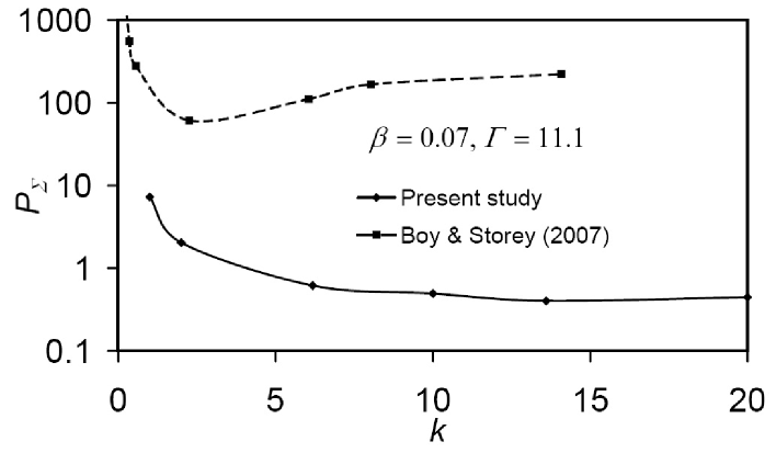
Figure 5: The marginal stability curve of $P_{\Sigma}$ vs. $k$ for $\beta$=0.07 and $\Gamma$=11.1.

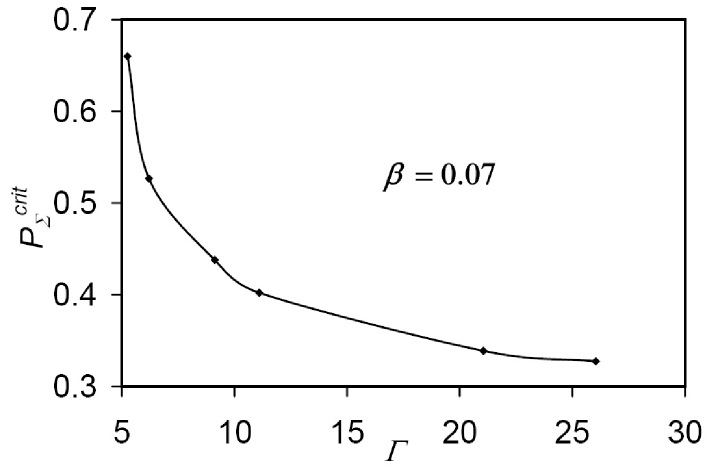
Figure 6: Plot of $P_{\Sigma}^{cri}$ vs. $\Gamma$ indicating critical conditions for the onset of instability at $\beta$=0.07.

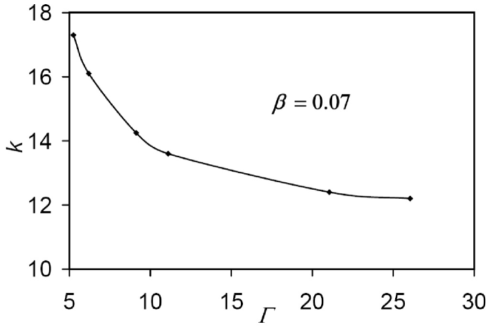
Figure 7: Plot of $k$ vs. $\Gamma$ at critical conditions for the onset of instability at $\beta$=0.07.

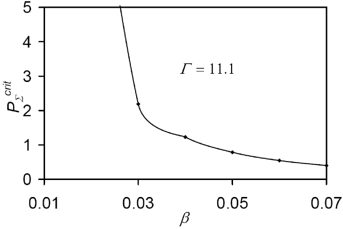
Figure 8: Plot of $P_{\Sigma}^{cri}$ vs. $\beta$ indicating critical conditions for the onset of instability at $\Gamma$=11.1.

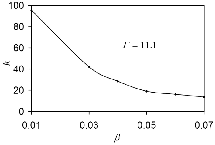
Figure 9: Plot of $k$ vs. $\beta$ at critical conditions for the onset of instability at $\Gamma$=11.1.

Figure (6) shows $P_{\Sigma}^{cri}$ vs. $\Gamma$ indicating the critical condition for the onset of instability at $\beta=0.07$. As expected, when $\Gamma$ increases the critical value of $P_{\Sigma}$ decreases. It implies that the system is more unstable with a larger conductivity ratio between the two liquids. The wavenumbers at the critical condition for instability, in this case, are plotted in Figure (7).

Figure (8) shows $P_{\Sigma}^{cri}$ vs. $\beta$ indicating the critical condition for the onset of instability at $\Gamma=11.1$. As $\beta$ decreases, i.e. as the channel becomes more shallow, the critical value of $P_{\Sigma}$ increases. It implies that the shallow nature of the channel has a stabilizing effect on the instability. The wavenumbers at the critical condition for instability, in this case, are plotted in Figure (9).

Finally, we compare the cases where the electric field is applied parallel or perpendicular to the liquid-liquid interface. Using the same parameters as those used in Figure (5), it was found that the critical electric field for the onset of instability for the parallel electric field case is $0.08kV/cm$ [1]. Comparing this with the value of $0.06kV/cm$ computed above for the perpendicular electric field case, it is implied that the perpendicular electric field case is more unstable. Although we have compared these numbers at the experimentally relevant condition, this trend continues at other parameters.

4 Discussion

Some comments pertaining to the problem formulation and future experiments are in order. These issues are discussed below.

In this work we have assumed that there is no electroosmotic flow. Similar assumption has been made in the past by, e.g., Boy and Storey [11]. While electroosmotic flow can affect the instability, it has been reported in prior work that the influence is little when the ratio of electroosmotic to electroviscous velocity is small (see Lin et al. [3] and Chen et al. [5]). Instabilities caused by electroosmotic slip velocity have been studied by others (see Boy and Storey [11] for references). As noted by Boy and Storey [11], such instabilities do not rely upon bulk conductivity gradient and therefore occur by a different mechanism than the one considered in this work.

We have used a constant current condition in the base state with respect to which a linear stability analysis is done. The electrodes have a Dirichlet boundary condition which is similar to that used in prior analytic work [3, 4, 5, 6, 7, 11, 8]. Our work does not consider the charging of the double layer at the electrodes. Boy and Storey [11] note that “the double layer capacitance acts as a high-pass RC filter on the electric field in the bulk. Double layer charging simply adds another mechanism to reduce the instability.” Thus, our work helps establish a baseline with respect to which the effects of electrode charging can be studied in the future.

The analysis presented here is strictly valid only when the time scale of the growth rate is shorter than the diffusion time scale. Yet, this analysis is useful to understand the nature of the instability and its domain of unstable behavior. This has been discussed in our previous work (Patankar [1]), where thresholds for validity have been shown. Similar discussion is also reported by Boy and Storey [11].

In our analysis, the infinite domain case is considered as a reference case which would be relevant when the channel is very wide. In microfluidic scenarios, this may not be applicable. Hence, we have considered the shallow channel configuration, experiments for which can be set up according to the problem definition in the paper. This is no different from the analyses presented by Santiago and co-workers [3, 4, 5, 6, 7, 11, 8]. El Moctar et al. [13] have reported similar experiments but they have a square cross section channel instead of a shallow channel. Thus, direct comparison with their data is not feasible.

5 Conclusion

In this paper the instability at the interface between two miscible liquids with identical mechanical properties but different electrical conductivities was analyzed in the presence of a perpendicular electric field. Linear stability analysis was done by considering a sharp interface between adjacent liquids in the base state. This approach enabled an analytic solution for the critical condition of the electrokinetic instability. It was seen that the instability depends on a non-dimensional parameter $P_{\Sigma}$ defined in the Equation (30).

The mechanism of instability was analyzed. It was found that the electrohydrodynamic coupling due to the interface condition for the electrical conductivity and the electrical body force in the fluid equations led to the instability.

The perpendicular electric field case is more unstable compared to the parallel electric field case. The reason for this is the greater asymmetry in the perpendicular field case that results in larger destabilizing electrohydrodynamic force.

The effect of a microchannel geometry was studied and the relevant parameters were found to be $P_{\Sigma},\beta$, and $\Gamma$ as defined in the paper.

The analysis captured the threshold type behavior for the onset of instability. It showed that larger conductivity ratio has a destabilizing effect, while the shallow nature of the channel has a stabilizing effect on the instability. Our approach provides a theoretical estimate and scaling for the desired parameters.

References

- [1] NA Patankar. Electrokinetic instability: The sharp interface limit. PHYSICS OF FLUIDS, 23(1):014101, JAN 2011.
- [2] MH Oddy, JG Santiago, and JC Mikkelsen. Electrokinetic instability micromixing. ANALYTICAL CHEMISTRY, 73(24):5822–5832, DEC 15 2001.
- [3] H Lin, BD Storey, MH Oddy, CH Chen, and JG Santiago. Instability of electrokinetic microchannel flows with conductivity gradients. PHYSICS OF FLUIDS, 16(6):1922–1935, JUN 2004.
- [4] MH Oddy and JG Santiago. Multiple-species model for electrokinetic instability. PHYSICS OF FLUIDS, 17(6):064108, JUN 2005.
- [5] CH Chen, H Lin, SK Lele, and JG Santiago. Convective and absolute electrokinetic instability with conductivity gradients. JOURNAL OF FLUID MECHANICS, 524:263–303, FEB 10 2005.
- [6] BD Storey, BS Tilley, H Lin, and JG Santiago. Electrokinetic instabilities in thin microchannels. PHYSICS OF FLUIDS, 17(1):018103, JAN 2005.
- [7] JD Posner and JG Santiago. Convective instability of electrokinetic flows in a cross-shaped microchannel. JOURNAL OF FLUID MECHANICS, 555:1–42, MAY 25 2006.
- [8] H Lin, BD Storey, and JG Santiago. A depth-averaged electrokinetic flow model for shallow microchannels. JOURNAL OF FLUID MECHANICS, 608:43–70, AUG 10 2008.
- [9] A. Kerem Uguz, O. Ozen, and N. Aubry. Electric field effect on a two-fluid interface instability in channel flow for fast electric times. PHYSICS OF FLUIDS, 20(3):031702, MAR 2008.
- [10] A. Kerem Uguz and N. Aubry. Quantifying the linear stability of a flowing electrified two-fluid layer in a channel for fast electric times for normal and parallel electric fields. PHYSICS OF FLUIDS, 20(9):092103, SEP 2008.
- [11] DA Boy and Storey BD. Electrohydrodynamic instabilities in microchannels with time periodic forcing. PHYSICS REVIEW E, 76:026304, 2007.
- [12] J. R. Melcher. Continuum Electromechanics. MIT Press, 1981.
- [13] El Moctar AO, Aubry N, and Batton J. Electro-hydrodynamic micro-fluidic mixer. LAB CHIP, 3:273–280, 2003.