Heliostat blocking and shadowing efficiency in the video-game era

Abstract

Blocking and shadowing is one of the key effects in designing and evaluating a thermal central receiver solar tower plant. Therefore it is convenient to develop efficient algorithms to compute this effect. In this paper we explore the possibility of using very efficient clipping algorithms developed for the video game and imaging industry to compute the block and shadowing efficiency of a solar thermal plant layout. We propose an algorithm valid for arbitrary position, orientation and size of the heliostats. This algorithm turns out to be very accurate and fast. We show the feasibility of the use of this algorithm to the optimization of a solar plant by studying a couple of examples in detail.

1 Introduction

Blocking and shadowing efficiency is one of the main sources of losses in a field design. Modern plants may have thousands of heliostats, and this blocking and shadowing efficiency should be computed for each of the heliostats. Nevertheless an efficient computation of these effects is non trivial. It depends not only on the characteristics of the receiver, but also on the position and orientation of each of the heliostats. This makes the computation depend on the date and time.

Methods based on ray-tracing techniques achieve a high accuracy on the estimation of the shadow and block effects, but at a high cost in computation time. This makes this type of approach unfeasible for optimization, where we have to evaluate the efficiency of plants with thousands of heliostats thousands of times.

A second method to estimate these block and shadow effects is based in some kind of tessellation of the heliostat (see for example Elsayed and Fathalah (1986); Leonardi and D’Aguanno (2011)). In this approach the heliostat is divided in pieces, and then a check is performed to see if each of these pieces is shadowed or blocked by the rest of the heliostat field. This approach can in principle achieve an arbitrary precision by refining the tessellation, but again at the price of a high computational cost.

A third and practical method used in plant optimization consists in developing some special formulas for the cases under study, that work under certain assumptions. Usually one assumes that the heliostat is blocked and shadowed by other heliostats that are parallel to it, and neglect the possibility that the same part of the heliostat is blocked/shadowed by more than one heliostat. While one can argue that these approximations are accurate enough for the practical purpose of optimizing a field layout, they clearly may have an impact difficult to quantify on the optimal design. Moreover, modern large plants benefit from having more than one tower (see for example Crespo and Ramos (2009)), and therefore some assumptions may be blatantly violated, since heliostats aiming at different towers are not parallel at all.

It would, therefore, be ideal if one could have an algorithm for evaluating blocking and shadowing effects that meets the following criteria:

• Being fast enough that it can be used in optimization process.

• Being very precise and free of assumptions, working for arbitrary positions/orientations of heliostats in a possibly non flat ground.

In our opinion none of the previous approaches meet these strict criteria. Most of the previous approaches to the problem of evaluating blocking and shadowing efficiencies date back to the first steps of tower solar plants, around the late 70’s and 80’s. But the area of computer graphics has evolved tremendously since then. Computer video games depend crucially on efficient clipping strategies (determining what portion of a “picture” covers some region) to be able to render scenes with high visual quality.

From the purely algorithmic point of view, computing the blocking and shadowing efficiency is nothing more than a clipping problem. More specifically, we have to determine which portion of the subject heliostat is visible both from the sun and the receiver point of view. In this work we apply an efficient 2D polygon clipping algorithm to the problem of computing the blocking and shadowing heliostat efficiency. The algorithm will prove to be extremely fast, and works for arbitrary shapes, positions, sizes and orientations of the heliostats (in particular it is as difficult to evaluate for a non flat ground as for a flat one). It also takes into account correctly the possibility that part of the blocked/shadowed region may be common to several heliostats. The only assumption made is that the heliostat is flat. Since modern heliostats are canted to the slant range the error made with this approximation is smaller than 1 part in $10^{5}$ (and, in practice, probably smaller), and therefore completely negligible. In this way we achieve our goal of a fast, precise and assumption-free algorithm to evaluate blocking and shadowing efficiency.

The paper is organized as follows: Section 2 contains our choice of notation and coordinate systems used for the computations, as well as some information about polygons, that are a crucial element in our algorithm. Section 3 contains a detailed description of our algorithm, while section 4 contains some examples of our algorithm in use. We finally conclude in section 5.

2 Generalities

2.1 Coordinate systems

Vectors are represented with an arrow $\vec{v}$, and their components by indices $\vec{v}=(v_{x},v_{y},v_{z})$. We will use different coordinate systems. One is the local coordinate system of the plant, with the positive $X$ axis pointing to the north, the positive $Y$ axis pointing to the West and the $Z$ axis being the height. In this reference system ($S=XYZ$) the sunlight direction is given by the unit vector

$$\vec{u}_{s}=(-\cos\eta\cos\theta,\cos\eta\sin\theta,-\sin\eta)$$ (1)

where $\eta$ is the solar height and $\theta$ is the azimuth measured from the north point. We will consider flat heliostats, and define a coordinate system for each heliostat, denoted $S^{\prime}_{h}=X^{\prime}Y^{\prime}Z^{\prime}$. It has the origin in the center of the heliostat, and the $Z^{\prime}$ axis being the normal to the heliostat, and the positive direction in the direction of the reflected light. The $S^{\prime}_{h}$ coordinate system is completely determined by saying that the $X^{\prime}$ axis forms an angle $\phi$ with the $XY$ plane. Obviously the coordinates of the corners of a flat heliostat $h$ in the coordinate system $S_{h}^{\prime}$, denoted by $\vec{P}^{\prime a}$ with $a=1,\dots,N_{c}$ ($N_{c}$ is the number of corners of the heliostat), are given by

$$\vec{P}^{\prime 1} = (P^{\prime 1}_{x},P^{\prime 1}_{y},0)$$

$$\vec{P}^{\prime 2} = (P^{\prime 2}_{x},P^{\prime 2}_{y},0)$$ (2)

$$\vdots$$

and in the particular case of a rectangular heliostat with dimensions $L_{x}\times L_{y}$ we have

$$\vec{P}^{\prime 1} = (-L_{x}/2,L_{y}/2,0)$$

$$\vec{P}^{\prime 2} = (-L_{x}/2,-L_{y}/2,0)$$

$$\vec{P}^{\prime 3} = (L_{x}/2,-L_{y}/2,0)$$

$$\vec{P}^{\prime 4} = (L_{x}/2,L_{y}/2,0)\,.$$ (3)

If $\vec{u}_{t}$ is the unit vector that points from the heliostat to the receiver the normal of the heliostat defining the $Z^{\prime}$ axis is given by

$$\vec{n}=\vec{u}_{t}-\vec{u}_{s}$$ (4)

that can be used to transform from one coordinate system to the other. Defining a rotation matrix using the Euler angles in the $ZXZ$ convention

$$R(\alpha,\beta,\gamma) = \left(\begin{array}[]{ccc}\cos\gamma&\sin\gamma&0\\ -\sin\gamma&\cos\gamma&0\\ 0&0&1\\ \end{array}\right)$$ (8)

$$\times \left(\begin{array}[]{ccc}1&0&0\\ 0&\cos\beta&\sin\beta\\ 0&-\sin\beta&\cos\beta\\ \end{array}\right)$$ (12)

$$\times \left(\begin{array}[]{ccc}\cos\alpha&\sin\alpha&0\\ -\sin\alpha&\cos\alpha&0\\ 0&0&1\\ \end{array}\right)$$ (16)

the application that transform between coordinate systems is given by

$$T_{h} : S\longrightarrow S^{\prime}_{h}$$

$$\vec{x}^{\prime} = T_{h}(\vec{x})=\tilde{R}_{h}\left(\vec{n},\phi\right)(\vec{x}-\vec{P})$$ (17)

where $\vec{P}$ is the position of the center of the heliostat, $\vec{n}$ a vector normal to the heliostat and

$$\tilde{R}_{h}\left(\vec{n},\phi\right)=R\left(\arctan\frac{n_{1}}{-n_{2}},\arctan\frac{\sqrt{n_{1}^{2}+n_{2}^{2}}}{n_{3}},\phi\right).$$ (18)

It is also straightforward to write the form of the inverse transformation

$$T^{-1}_{h} : S^{\prime}_{h}\longrightarrow S$$

$$\vec{x} = T^{-1}_{h}(\vec{x}^{\prime})=\tilde{R}^{T}_{h}\left(\vec{n},\phi\right)\vec{x}^{\prime}+\vec{P}$$ (19)

that can be used to obtain the coordinates of the corners of an heliostat in the $S$ coordinate system

$$\vec{P}^{a}=T^{-1}_{h}(\vec{P}^{\prime a})\,.$$ (20)

2.2 Polygons

We will make extensive use of simple polygons in the following discussion. We will represent a polygon by giving the $N_{c}$ coordinates of the corners, and use calligraphic letters to identify them. For example if $\vec{P}^{a}$ with $a=1,\dots,4$ are the four corners of an heliostat, they form the polygon $\mathcal{P}=\vec{P}^{1}\vec{P}^{2}\vec{P}^{3}\vec{P}^{4}$. We can have polygons in the plane, in which case the corners are 2D points, or we can have them in space, in which case the points have three components and it is assumed that all corners lay on a common plane.

In the case of 2D polygons, we will write $\vec{x}\in\mathcal{P}$ when the point $\vec{x}$ is inside the polygon $\mathcal{P}$ and $\vec{x}\notin\mathcal{P}$ otherwise. There is a very efficient algorithm to determine if a point lies inside a polygon based on Jordan’s curve theorem, called the even-odd rule. One draws a straight line from the point $\vec{x}$ to the infinity (in an arbitrary direction) and count how many times it crosses the polygon $\mathcal{P}$. The point is inside the polygon if and only if this counting is an odd number. We use simulation of simplicity (SoS) techniques to deal with the possible degenerate cases (Edelsbrunner and Mücke, 1990).

One can define the union, intersection and difference of 2D polygons, being each of them one or more polygons. The following definitions are straightforward

$$\mathcal{A}=\mathcal{B}\cup\mathcal{C} \Longleftrightarrow \left\{\vec{x}\in\mathcal{A}\Longrightarrow\vec{x}\in\mathcal{A}\textrm{ or }\vec{x}\in\mathcal{B}\right\}$$

$$\mathcal{A}=\mathcal{B}\cap\mathcal{C} \Longleftrightarrow \left\{\vec{x}\in\mathcal{A}\Longrightarrow\vec{x}\in\mathcal{A}\textrm{ and }\vec{x}\in\mathcal{B}\right\}$$

$$\mathcal{A}=\mathcal{B}\setminus\mathcal{C} \Longleftrightarrow \left\{\vec{x}\in\mathcal{A}\Longrightarrow\vec{x}\in\mathcal{A}\textrm{ and }\vec{x}\notin\mathcal{B}\right\}.$$ (21)

3 Efficient computation of blocking and shadowing efficiency and clipping algorithm

3.1 General idea

Given a subject heliostat (denoted $c$), we have to determine the fraction of reflecting surface that is not shadowed or blocked by a set of heliostats (denoted $h^{(i)}$ with $i=1,\dots,N$). For the sake of simplicity in what follows we will assume that the heliostats are rectangular with lengths $L_{x}$ and $L_{y}$. The generalization to the case of different lengths for different heliostats or different shapes is straightforward and will be discussed later.

Our proposed algorithm works in three phases:

1. Project each of the corners of each heliostat $h^{(i)}$ to the subject’s heliostat plane. When doing this projection from the sun point of view we will determine the shadowing, and when doing it from the tower point of view we will determine the blocking.

   After this first phase we have $2N$ quadrilaterals in the subject’s heliostat plane.

2. Compute the set-theoretical difference between the subject heliostat and the $2N$ quadrilaterals. This is basically a 2D polygon clipping problem that can be solved very efficiently.

   After this second stage we have one polygon (in the general case we can have more than one) that represents the effective reflecting surface of the heliostat.

3. The shadowing and blocking efficiency is simply the result of the ratio between the effective reflective surface and the total area of the heliostat.

Now we will describe in detail each of these three steps.

3.2 Projection to the heliostat plane

We will consider a square heliostat $c$ of dimensions $L_{x}\times L_{y}$ whose corners have coordinates in the plant reference system $P^{a}_{c}$ with $a=1,2,3,4$. As we have mentioned the coordinates of these corners in the reference system ($S_{c}^{\prime}$) associated to the heliostat $c$ are given by Eqs. 2.1, and these can be transformed to the plant reference system using Eq.19.

To compute the shadowing losses on an heliostat $c$ we have to determine the intersection of the line that passes through each of the heliostat corners with direction $\vec{u}_{s}$ (given by Eq. 1) with the plane of the subject heliostat, defined by having a normal direction $\vec{n}_{c}$ and passing by the center of the heliostat $\vec{X}_{c}$. In this case the intersection points, labeled $\vec{s}^{a}$, are easily determined by

$$\vec{s}^{a}=\vec{P}^{a}_{c}+\left(\frac{\vec{n}_{c}\cdot\vec{X}_{c}-\vec{n}_{c}\cdot\vec{P}^{a}_{c}}{\vec{n}_{c}\cdot\vec{u}_{s}}\right)\vec{u}_{s}\,.$$ (22)

In order to compute the blocking losses one has to proceed in a similar way, but replacing the role of the sun with the role of the receiver. In this case we have to compute the intersection of the lines that pass through the heliostat corners and the receiver at which each heliostat is aiming (in the general case of a multi-tower or multi-receiver plant, different heliostats may aim at different points). Let us denote the position of the receiver in the plant reference system with $\vec{T}$. Then, after defining the unit vectors

$$\vec{u}^{a}_{t}=\frac{\vec{T}-\vec{P}^{a}_{c}}{|\vec{T}-\vec{P}^{a}_{c}|}\,,$$ (23)

the intersection points needed to compute the blocking are given by

$$\vec{b}^{a}=\vec{P}^{a}_{c}+\left(\frac{\vec{n}_{c}\cdot\vec{X}_{c}-\vec{n}_{c}\cdot\vec{P}^{a}_{c}}{\vec{n}_{c}\cdot\vec{u}_{t}^{a}}\right)\vec{u}_{t}^{a}\,.$$ (24)

The situation where $\vec{n}_{c}\cdot\vec{u}_{t}^{a}=0$ (or $\vec{n}_{c}\cdot\vec{u}_{t}=0$) represents heliostats laying perpendicular one to the other, either from the tower (or sun) point of view. Since in thiss case there is no blocking (or shadowing), one can discard these situations immediately without any need of computing any projection.

Figure 1: This figure shows the subject heliostat $c$ in the reference system defined by itself ($S^{\prime}_{c}$). The heliostats that can potentially contribute to the losses of the heliostat $c$ define a set of quadrilaterals in this reference system via Eqs. 22 and 24. If any of the these quadrilaterals have all the corners at the right of the heliostat (i.e. the $x$ coordinate of all corners is larger than $L_{x}/2$), then we know that it can not contribute to the heliostat losses. The same principle applies when the corners are to the left, top or bottom.

Each set of points ${\vec{s}^{a}}$ and ${\vec{b}^{a}}$ determines a quadrilateral in the heliostat plane, and therefore in the $S^{\prime}_{h}$ reference system all these points have a zero value for the third component. Therefore the first two components of the vectors $\vec{s}^{\prime a}=T_{c}(\vec{s}^{a})$ and $\vec{b}^{\prime a}=T_{c}(\vec{b}^{a})$ define 2D polygons $\mathcal{S}=\vec{s}^{\prime 1}\vec{s}^{\prime 2}\vec{s}^{\prime 3}\vec{s}^{\prime 4}$ and $\mathcal{B}=\vec{b}^{\prime 1}\vec{b}^{\prime 2}\vec{b}^{\prime 3}\vec{b}^{\prime 4}$.

This process is repeated for each of the heliostats $h^{(i)}$, giving a total of $2N$ polygons, that we will denote $\mathcal{S}_{i}$ and $\mathcal{B}_{i}$ with $i=1,\dots,N$.

Note that at this stage we can already eliminate many contributions to the heliostat losses. If any of the 2D polygons $\mathcal{S}_{i}$ or $\mathcal{B}_{i}$ have the four corners in the $S^{\prime}_{c}$ reference system in the same region (labelled $I,II,III$ and $IV$ in Fig. 1), then this polygon can not be the source of field losses and one can immediately discard it.

3.3 2D polygon clipping

Our subject heliostat defines a polygon in his $S^{\prime}_{c}$ reference system given by $\mathcal{C}=\vec{P}^{\prime 1}\vec{P}^{\prime 2}\vec{P}^{\prime 3}\vec{P}^{\prime 4}$. The total reflecting area $\mathcal{R}$ is given by

$$\mathcal{R}=\mathcal{C}\setminus\left(\cup_{i=1}^{N}\mathcal{S}_{i}\cup\mathcal{B}_{i}\right)$$ (25)

This defines our clipping problem. There are several ways to proceed, but probably the most effective consists in defining $\mathcal{R}=\mathcal{C}$, and then iteratively subtract to $\mathcal{R}$ the polygons $\mathcal{B}_{1},\mathcal{S}_{1},\mathcal{B}_{2},\mathcal{S}_{2},\dots$ See algorithm 1.

1:  Compute $\mathcal{S}_{i},\mathcal{B}_{i}$ for each heliostat $i=1,\dots,N_{h}$ {Use Eqs. 22 and 24}

2:  Start $\mathcal{R}=\mathcal{C}$

3:  for $n=1$ to $N_{h}$ do

4:     $\mathcal{R}\leftarrow\mathcal{R}\setminus\mathcal{B}_{n}$

5:     $\mathcal{R}\leftarrow\mathcal{R}\setminus\mathcal{S}_{n}$

6:  end for

7:  return  $\textrm{Area}(\mathcal{R})/\textrm{Area}(\mathcal{C})$ {Use shoelace formula to compute area of polygons.}

Algorithm 1 Algorithm to compute block and shadow

To compute efficiently the blocking and shadowing effects it is crucial to have an efficient algorithm to perform the 2D polygon clipping (in particular, the polygon set difference). The algorithm should be valid for arbitrary simple polygons. In principle all the polygons $\mathcal{C}$, $\mathcal{B}_{i}$ and $\mathcal{S}_{i}$ are convex polygons, but after subtracting some portions of a polygon the result will in general be a non-convex polygon. In particular we choose (Greiner and Hormann, 1998) and the interested reader should consult the original reference. Being a crucial step in our implementation, we will give an overview of how the algorithm works in section 3.5

3.4 Final computation

At this point we have a polygon representing the portion of the subject heliostat that is visible both from the point of view of the sun and the point of view of the tower, and this is precisely the effective reflecting surface. The final efficiency of the subject heliostat is given by the area of the reflecting surface over the total area of the heliostat.

The so called shoelace formula gives the area of an arbitrary simple 2D polygon. If the corners are $\mathcal{P}=\left\{\vec{P}^{a};a=1,\dots,N_{c}\right\}$, the area is given by

$$A(\mathcal{P})=\frac{1}{2}\sum_{a=1}^{N}\left(P_{x}^{a}P_{y}^{a+1}-P_{x}^{a+1}P_{y}^{a}\right)\,,$$ (26)

with $P_{x}^{N+1}=P_{x}^{1}$ and $P_{y}^{N+1}=P_{y}^{1}$. The sign of the area given by the previous formula gives the orientation of the polygon. If the points are labeled in counterclockwise direction the sign is positive and negative otherwise, but the absolute value always represents the area of the polygon.

A simple application of the previous formula gives the blocking and shadowing efficiency

$$e=\frac{A(\mathcal{R})}{A(\mathcal{C})}\,.$$ (27)

3.5 Clipping algorithm

The clipping algorithm basically works in three phases. We will refer to Fig 2 as an example, where one wants to compute the difference between the polygons $\mathcal{A}=\{\vec{a}_{1}\vec{a}_{2}\vec{a}_{3}\vec{a}_{4}\}$ and $\mathcal{B}=\{\vec{b}_{1}\vec{b}_{2}\vec{b}_{3}\vec{b}_{4}\}$.

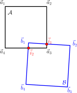
Figure 2: Example of polygon clipping. Given two polygons $\mathcal{A}=\{\vec{a}_{1}\vec{a}_{2}\vec{a}_{3}\vec{a}_{4}\}$ and $\mathcal{B}=\{\vec{b}_{1}\vec{b}_{2}\vec{b}_{3}\vec{b}_{4}\}$, to determine the difference between the two polygons $\mathcal{A}\setminus B$ we have first to determine the intersection points, labeled $\vec{i}_{1}$ and $\vec{i}_{2}$. The final result is the polygon $\mathcal{A}\setminus\mathcal{B}=\{\vec{i}_{1}\vec{b}_{1}\vec{i}_{2}\vec{a}_{4}\vec{a}_{1}\vec{a}_{2}\}$.

One starts by determining the intersection points between the two polygons. In our example there are two of them, and we label them $\vec{i}_{1}$ and $\vec{i}_{2}$. These are inserted in both polygons that now become

$$\mathcal{A}=\{\vec{a}_{1}\vec{a}_{2}\vec{i}_{1}\vec{a}_{3}\vec{i}_{2}\vec{a}_{4}\}$$ (28)

and

$$\mathcal{B}=\{\vec{b}_{1}\vec{i}_{1}\vec{b}_{2}\vec{b}_{3}\vec{b}_{4}\vec{i}_{2}\}\,.$$ (29)

The intersection points in each polygon are marked to record if they are entry or exit points to the other polygon’s interior. In our example we have

$$\mathcal{A}=\{\vec{a}_{1}\vec{a}_{2}\vec{i}_{1}^{\rm entry}\vec{a}_{3}\vec{i}_{2}^{\rm exit}\vec{a}_{4}\}$$ (30)

and

$$\mathcal{B}=\{\vec{b}_{1}\vec{i}_{1}^{\rm exit}\vec{b}_{2}\vec{b}_{3}\vec{b}_{4}\vec{i}_{2}^{\rm entry}\}\,.$$ (31)

Finally we have to trace the clipped polygon $\mathcal{A}\setminus\mathcal{B}$. The method is quite simple, one starts in an intersection point (say for example $\vec{i}_{1}$) and moves to the interior of polygon $\mathcal{A}$ following polygon $\mathcal{B}$. When one arrives to another intersection point, one has to switch polygons: we will follow polygon $\mathcal{A}$ moving to the exterior of polygon $\mathcal{B}$. In our example this procedure leads to $\mathcal{A}\setminus\mathcal{B}=\{\vec{i}_{1}\vec{b}_{1}\vec{i}_{2}\vec{a}_{4}\vec{a}_{1}\vec{a}_{2}\}$, that as the reader can see traces the final polygon $\mathcal{A}\setminus\mathcal{B}$.

4 Tests and benchmarks

4.1 A simple case

As a simple test of our method we will consider a solar plant located at a latitude of $40.08^{\underline{\rm o}}$ with a receiver situated at $100$m of height. We will compute the blocking and shadowing efficiency of an heliostat $c$ at position

$$c\equiv(108,0,5)\,{\rm m}\,.$$ (32)

This heliostat is surrounded by two heliostats $h_{1}$ and $h_{2}$ with positions

$$h_{1} \equiv (100,8,5)\,{\rm m}\,,$$ (33)

$$h_{2} \equiv (100,-8,5)\,{\rm m}\,.$$ (34)

We will assume that all heliostats have dimensions $10\,{\rm m}\times 10\,{\rm m}$.

This example shows nicely how our algorithm can cope with very complex situations in which the blocking and shadowing effects of several heliostats overlap. We want to stress that this situation may happen in real optimal field designs, and that for sure this happens very often during an optimization process, where the design might be far from optimal.

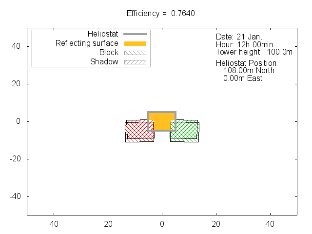
Figure 3: The subject heliostat $c$ and the projection of the shadow and block from heliostats $h_{1}$ (orange) and $h_{2}$ (blue) at noon. The blocking and shadowing efficiency of the heliostat $c$ is $0.76$. As the reader can see, both heliostats contribute to the total blocking and shadowing efficiency of the heliostat $c$.

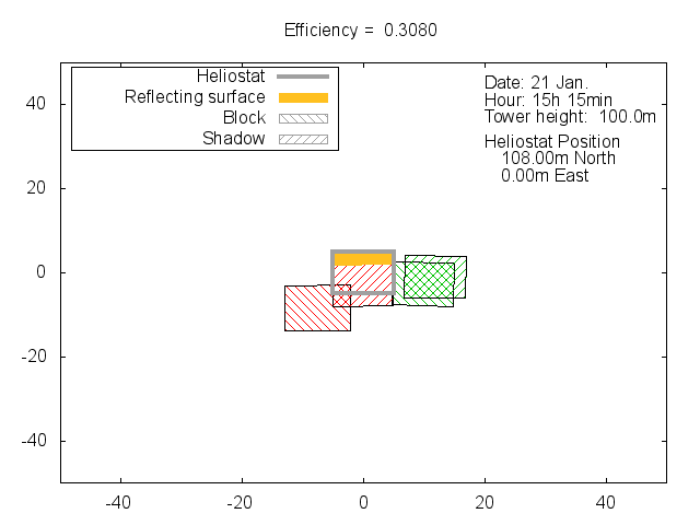
Figure 4: The subject heliostat $c$ and the projection of the shadow and block from heliostats $h_{1}$ (orange) and $h_{2}$ (blue). The blocking and shadowing efficiency of the heliostat $c$ is $0.31$. Both heliostats contribute to the total blocking and shadowing efficiency of the heliostat $c$, but there is some overlap between the blocking of heliostat $h_{1}$ and the shadowing of heliostat $h_{2}$.

Figure 3 shows the situation at 12h of the 21^st of January. As the reader can see both heliostats $h_{1}$ and $h_{2}$ contribute to the losses by the same amount due to the symmetric position of the heliostats relative to the receiver and the sun. There is also a large overlap between the blocked and the shadowed surface of both heliostats.

Figure 4 shows the same case at 15h 15min of the 21^st of January. Again both heliostats $h_{1}$ and $h_{2}$ contribute to the blocking and shadowing efficiency of heliostat $c$. But in this case the contributions of both heliostats are very different. Most of the effect comes from the shadowing effects of heliostat $h_{2}$ while heliostat $h_{1}$ only blocks a small portion of heliostat $c$. Moreover part of this blocking overlaps with the shadowing effect of heliostat $h_{2}$.

As the reader can observe our algorithm deals with these complicated situations easily and without any particular constrains. It is as easy to deal with these cases as to deal with the easy ones in which all the blocking and shadowing effect comes from a single heliostat.

4.2 A real scenario

As a more realistic example we will consider in detail the computation of the blocking and shadowing efficiency of one heliostat of a plant. The field layout was produced along the lines of (Ramos and Ramos, 2012). An overview of the complete field layout with the chosen heliostat for the computation of the blocking and shadowing efficiency can be seen in figure 5. In this example the plant is located at $38.23^{\underline{\rm o}}$ of latitude and the receiver is located at $150\,{\rm m}$ of height. All heliostats have dimensions $12.88\,{\rm m}\times 9.489\,{\rm m}$.

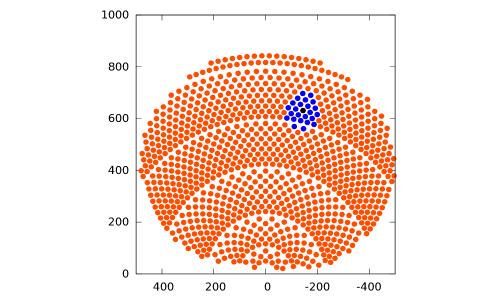
Figure 5: Field layout of a solar plant of 25Mwe with a $150\,m$ tower. The heliostat marked in black is the subject heliostat that we will use to demonstrate our algorithm located at $(630.93,-144.41,5)\,{\rm m}$. In blue are marked the 24 heliostats that are closer to the subject heliostat, and therefore the ones that are susceptible of affecting the efficiency of the subject heliostat.

We will study in detail the blocking and shadowing efficiency of an heliostat $c$ located at $(630.93,-144.41,5)\,{\rm m}$. For the sake of clarity we will only display the 24 heliostats (of the 1000 that are in the plant) that are closest to the subject heliostat. These are the ones that at some moments of the day affect the blocking and shadowing efficiency and are listed in Table 1. We stress that this limitation is only applied to avoid displaying 999 heliostats in the following figures, and that the real algorithm, as it is implemented, computes the effect of all heliostats of the plant.

n${}^{\underline{o}}$	Position [m] $(\vec{X}_{c})$	n${}^{\underline{o}}$	Position [m] $(\vec{X}_{c})$
1	(614.21, -126.29, 5.00)	13	(660.03, -105.31, 5.00)
2	(607.84, -153.31, 5.00)	14	(585.22, -161.42, 5.00)
3	(647.73, -163.37, 5.00)	15	(664.56, -183.31, 5.00)
4	(654.50, -134.57, 5.00)	16	(678.53, -123.87, 5.00)
5	(623.77, -172.05, 5.00)	17	(615.45, -199.18, 5.00)
6	(636.90, -116.27, 5.00)	18	(641.64, -87.72, 5.00)
7	(591.95, -135.48, 5.00)	19	(689.94, -174.02, 5.00)
8	(672.18, -153.84, 5.00)	20	(697.15, -143.34, 5.00)
9	(600.33, -179.84, 5.00)	21	(577.40, -186.87, 5.00)
10	(619.41, -98.828, 5.00)	22	(602.03, -82.30, 5.00)
11	(639.74, -191.65, 5.00)	23	(560.90, -146.37, 5.00)
12	(597.56, -109.09, 5.00)	24	(569.25, -110.83, 5.00)

Table 1: Position of the centers (denoted by $\vec{X}_{c}$ in the text) of the 24 heliostats of the power plant closer to the subject heliostat. These heliostats are marked in blue in figure 5.

We choose the 21${}^{\underline{\rm st}}$ of January as the date to display our results. Figures 6, 7 and 8 show the blocking and shadowing at different times of the day. At 8h (Fig. 6) in the morning (fig. 6) the efficiency is around $0.86$, and two heliostats contribute to the losses. At 12h (Fig. 7) only the blocking of one heliostat contribute to the losses and the efficiency is $0.96$. Finally at 16h 15m (Fig. 8) the situation becomes more complex, since several heliostats contribute to the losses with some overlap between the blocking and shadowing effects. In this last case the final efficiency drops to $0.52$.

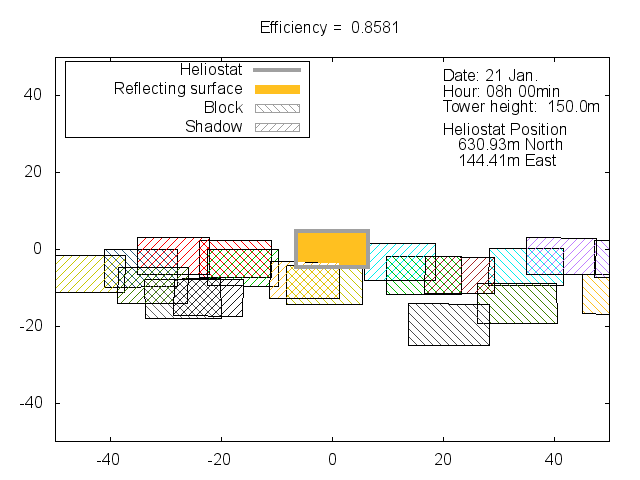
Figure 6: Blocking and shadowing efficiency of an heliostat in a real plant situation. At 8h the efficiency is $0.86$. In this partiular case two different heliostats produce shadowing losses, and one produce some blocking.

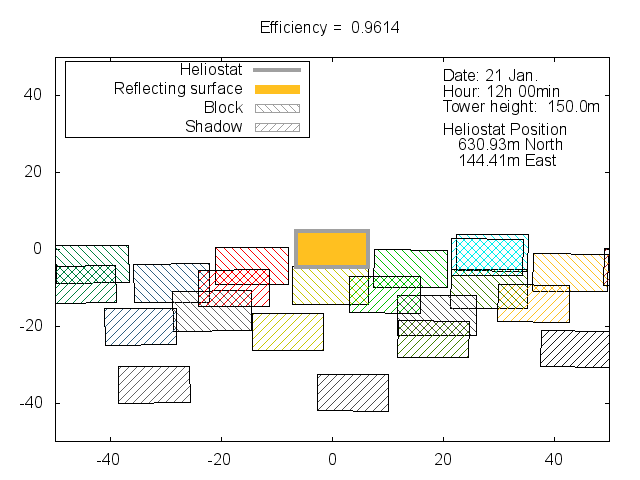
Figure 7: Blocking and shadowing efficiency of an heliostat in a real plant situation. At 12h the efficiency is $0.96$, with only one heliostat contributing to the losses.

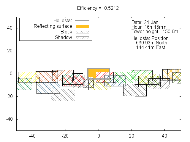
Figure 8: Blocking and shadowing efficiency of an heliostat in a real plant situation. At 16h 15min several heliostats contribute to the losses and the efficiency drops to $0.52$. This situation is quite complex, since there is some overlapping between the blocking and shadowing of several heliostats.

From this realistic example we get some important lessons. First, it is fairly difficult that very many heliostat contribute to the losses (except just at sunrise or at sunset), and therefore most of the heliostats of the plant can be easily discarded from the computation after the first step described in section 3.2. This step can be implemented regardless of the algorithm that is used afterwards for the blocking and shadowing efficiency. Second, it is common, even in an optimized field layout, that various heliostats contribute to the blocking and shadowing efficiency, and that there is some overlap from the contribution of several heliostats. Third, the heliostats that contribute to the losses change with the position of the sun. Our algorithm deals smoothly with these complicated but common situations.

4.3 Benchmarks

We have implemented the algorithm previously described in FORTRAN. For an optimal performance we recommend to use a linked list to describe polygons in order to avoid moving/copying data when inserting or removing points from polygons. The original reference (Greiner and Hormann, 1998) contains a detailed description of such data structures (in C).

As a benchmark we have used the same field layout shown in figure 5. This field consists of 1000 heliostats, and we have measured the time needed to compute the blocking and shadowing efficiency of each heliostat. Since this time is very small, we have repeated the computation 100 times and quote the average as our final value.

Hour	Execution Time	Field efficiency (Average)
8h 00min	517 ms	0.747
12h 00min	527 ms	0.975
16h 15min	525 ms	0.899

Table 2: Times for the computation of the blocking and shadowing efficiency of each heliostat of the field shown in Fig. 5. For each heliostat we have taken into account the effect of the remainning 999 heliostats. Since the times are very small (around half a second), we have measured the time needed to compute 100 times the efficiency of all heliostats of the plant, and quote the average as our final result.

The results can be seen in Tab. 2. The quoted times refer to runs on a standard laptop (processor Intel Core(TM) i7-3687U CPU @ 2.10GHz). In summary we can say that, for a plant of a thousand heliostats, our algorithms computes the blocking and shadowing efficiency in around half a second. These times seem to be pretty independent on the date/time as long as the field layout is reasonable (i.e. close to optimal, or at least acceptable).

5 Conclusions

In this work we have developed a new algorithm to compute the heliostat blocking and shadowing efficiency. This algorithm is based on projecting the image of all heliostats of the field to the plane of the subject heliostat, both from the point of view of the sun (shadowing effect) and from that of the tower (blocking effect). This projected figures form a set of 2D polygons and our original problem of computing the blocking and shadowing efficiency is translated into a clipping problem of 2D polygons. This last problem can be solved very efficiently thanks to the efficient algorithms developed for the computer video game industry.

We have used one such algorithm (Greiner and Hormann, 1998) and showed that the shadowing and blocking efficiency can be computed very fast: our FORTRAN code uses less than one second to compute the blocking and shadowing efficiency of all 1000 heliostats of a plant running, on a standard laptop.

The algorithm has no restrictions. Heliostats can be of different sizes, or be located at different heights. They can aim at different towers and be located in completely arbitrary positions without any penalty in the time used by the algorithm to compute the efficiency. The algorithm is exact, and does not assume any particular geometry or property of the heliostats.

We have shown our algorithm at work in some detail for two particular cases: a simple case in which two heliostats are in front of another, and a more realistic example in which we have picked up an heliostat from a real optimal design of a 15MWe plant with 1000 heliostats. We also want to call the attention of the reader to two multimedia files Ramos and Ramos. ; Ramos and Ramos that show the blocking and shadowing efficiency for the two cases studied in this paper since the sunrise till the sunset.

In summary we think that the efficiency of our algorithm makes it a perfect choice for plant optimization where the blocking and shadowing efficiency has to be evaluated several thousands of times, while the lack of any particular assumptions and generality brings peace of mind to the results of such an optimization process.

6 Acknowledgments

The authors want to thank the help of S. Lottini for his comments and corrections after a careful reading of the manuscript.

Bibliography

Bibliography

- Crespo and Ramos (2009) Crespo, L., Ramos, F., 2009. NSPOC: A new powerful tool for heliostat field layout and receiver geometry optimizations, in: Proceedings of the SolarPACES 2009 conference, Berlin.
- Edelsbrunner and Mücke (1990) Edelsbrunner, H., Mücke, E.P., 1990. Simulation of Simplicity: A technique to cope with degenerate cases in geometric algorithms. ACM Transactions on Graphics 9(1), 66–104.
- Elsayed and Fathalah (1986) Elsayed, M.M., Fathalah, K.A., 1986. Estimation of percentage useful Area of a heliostat when considering shadowing and blocking. Solar & Wind Technology 3, 199.
- Greiner and Hormann (1998) Greiner, G., Hormann, K., 1998. Efficient clipping of arbitrary polygons. ACM Transactions on Graphics 17(2), 71.
- Leonardi and D’Aguanno (2011) Leonardi, E., D’Aguanno, B., 2011. CRS4-2: A numerical code for the calculation of the solar power collected in a central receiver system. Energy 36, 4828.
- (6) Ramos, A., Ramos., A., . Heliostat blocking and shadowing. (https://archive.org/details/nspoc_bands_564).
- (7) Ramos, A., Ramos, F., . Simple example of blocking and shadowing. https://archive.org/details/nspoc_bands_simple.
- Ramos and Ramos (2012) Ramos, A., Ramos, F., 2012. Strategies in tower solar power plant optimization. Solar Energy 86, 2536 – 2548. 1205.3059.