Strategies in tower solar power plant optimization.

Abstract

A method for optimizing a central receiver solar thermal electric power plant is studied. We parametrize the plant design as a function of eleven design variables and reduce the problem of finding optimal designs to the numerical problem of finding the minimum of a function of several variables. This minimization problem is attacked with different algorithms both local and global in nature. We find that all algorithms find the same minimum of the objective function. The performance of each of the algorithms and the resulting designs are studied for two typical cases.

We describe a method to evaluate the impact of design variables in the plant performance. This method will tell us what variables are key to the optimal plant design and which ones are less important. This information can be used to further improve the plant design and to accelerate the optimization procedure.

1 Introduction

One of the main tasks in the conversion of solar energy into electricity by solar power plants is to work out an optimized plant design. In this type of plant, the energy collector subsystems (heliostats, field receivers) represent a very important part of the cost break-down structure. Therefore, the use of detailed computer programs is of great interest in order to optimize the plant design.

The two main conceptual ingredients for a solar plant optimization code are:

1. Reduction of the plant design to the value of certain design variables.

2. An optimization criteria: This means having a function that computes the objective quantity (i.e. total annual power output, cost per produced power, etc…) as a function of the design variables. In general we will use the cost of the energy produced by the plant as the optimization criteria, and therefore use the terms optimize and minimize as interchangeable.

After the plant design is completed it becomes crucial to understand what role each of the design variables play in the optimal design. Some variables can be slightly moved away from the optimal value without impacting the plant performance while others can not be changed without a severe impact in the plant performance. We will give a precise definition of a quantity (we call it uncertainty) that will measure the importance of each variable in a plant design. We will give a precise mathematical definition of this uncertainty associated with a variable, and show how to compute these quantities for a general plant design.

The paper is organized as follows. In section 2 we will explain our choice of plant design variables. Sections 3 and 4 describe additional information needed to perform the optimization. We perform the numerical optimization using different algorithms, both global and local. Section 5 describes in detail the optimization procedure and our choice of three different algorithms: first we use a fast local optimizer especially designed to solve this problem, second we use complex optimization library that include a Monte-Carlo search, with the potential ability to jump over function barriers and find global optima. Finally we use a genetic algorithm, generally used for difficult optimizations and problems with a complex fitness landscape.

Section 6 attack the very important problem of determining what role each of the design variables have in the plant performance. As we will see, the Hessian of the objective function evaluated at the minimum will provide information on how flat each of the directions in the minimum are. This information will not only give us the uncertainty associated with each design variable, but also help us deciding if the function have several local optima and if the three algorithms have found the same design.

Finally, in section 7 we apply these optimization algorithms and analysis tools to two typical plant designs, and in section 8 we summarize our main results and present some perspectives for further studies.

2 Description of plant design variables

In choosing the variables that determine the layout of our plant, one has to take into account that an optimization procedure requires multiple evaluations of the objective function. Thus a proper choice of design variables must have the CPU cost of the optimization in mind.

In this section we will present our choice for plant design variables. This choice has been made with the following things in mind

• A plant should be circular-like to minimise the blocking and shadowing effect.

• Consecutive files of heliostats should be allocated in radial staggered position to minimise blocking and shadowing effect, and keep a compact field.

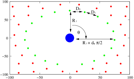
Figure 1: An example of the first two lines of heliostats in a field. The azimuthal angle starts in the north with the value $\theta=0$. In green we have the heliostats that belong to the first line. The distance of this line to the tower is given by $R_{1}$. The distance of all the lines $R_{n}$ is determined trough the recursion relation of Eq. 1. We see that this distance dependes on the azimuthal coordinate through the variable $d_{\theta}$ (Eq. 2). The azimuthal distance between heliostats of the first line ($D_{0}^{1},D_{1}^{1},\dots$) are determined through the recursive relation Eq. 3. The azimuthal position of the second and subsequent lines of heliostats is determined by positioning them at the average azimuthal position of the heliostats of the previous line (radial staggered) until a transition line is placed.

2.1 Collector field variables

The distance of the $n^{th}$ heliostat line to the tower ($R_{n}$) is given by the linear recursion formulae

$$R_{n}=a_{0}+(a_{1}+1)R_{n-1}$$ (1)

that defines the two variables

1. $a_{0}:$ Initial spacing between heliostat rows $[m]$.

2. $a_{1}:$ Increasing spacing between heliostat rows.

The recursion relation of Eq. 1 is solved by the condition $R_{0}=R_{\sc base}$ that specifies the distance between the tower and the first heliostat line. This space is usually used for operational purposes, like the administrative building, roads, etc…There is a minimal distance between heliostats $R_{\sc min}$ related with the size of the heliostats and some practical needs. $R_{n}$ is set to the maximum between the value given by the recursion relation of Eq. 1 and $R_{\sc min}$.

The shape of the lines of heliostats of an optimal field does not have to be perfectly circular. We consider the possibility of non circular shapes by adding to the previous radial distance an increment that dependes on the azimuthal position of the heliostat (we will call it $\theta$).

$$\Delta R=\left\{\begin{array}[]{lcl}d_{\theta}\theta&\textrm{for}&0<\theta\leq\pi\\ d_{\theta}(2\pi-\theta)&\textrm{for}&\pi<\theta<2\pi\\ \end{array}\right..$$ (2)

This defines another collector variable

1. $d_{\theta}:$ Correction of the radial distance with the azimuthal position.

Intuitively when $d_{\theta}>0$ the lines of heliostats will be closer to the tower in the north part of the field, whereas for $d_{\theta}<0$ heliostats will be closer to the tower in the south. Usually optimal designs are more compact in the south (and hence $d_{\theta}<0$) where there is less blocking and shadowing effect between heliostats.

A proper optimal layout should not only find the optimum radial spacing between heliostats of the same line, but also determine the azimuthal distance between them. We will use a similar technique than the one used for the radial distance. We need to determine how this azimuthal distance depends on both the azimuthal angle and the radial distance. If we call $D_{0}^{1}$ the azimuthal distance for the heliostat that is just in the north (zero azimuth) in the first line of heliostats, and number the heliostats in the same line with the index $\alpha=0,1,\dots$, the azimuthal distance as a function of the azimuthal angle $\theta$ is given by

$$D_{\alpha}^{1}=D_{\alpha-1}^{1}+e_{\theta}\theta$$ (3)

that, defines an additional variable

1. $e_{\theta}:$ Variation of the azimuthal distance with the azimuthal angle.

To start this recursion relation one should give $D_{0}^{1}$ as input. We will comment about this later.

Variable ([V04]) determine the azimuthal position only of the first line of heliostats. The remaining lines of heliostats are situated at the radial distance determined by the variables ([V01–V03]) and with radial staggered positions. This means that their azimuthal angle is the average of the azimuthal position of the two heliostats in front of it (see Fig. 1).

This rule of formation will increase azimuthal spacing between heliostats very fast. So it is convenient, after a certain amount of lines, to give an extra space and restart again the rule of formation forgetting the previous heliostats. This extra space increases with the distance to the tower. These re-starting lines are called transition lines, and heliostats between two transition lines are said to belong to the same group. The first line of heliostats of each group is at a distance from the previous heliostat line given by

$$\Delta=(1+a_{0}+a_{1}R)\delta+\epsilon$$ (4)

where $R$ is the last distance between lines given by Eq. 1. Eq. 4 defines two more optimization variables

1. $\epsilon:$ Extra distance for transition lines.

2. $\delta:$ Increment of distance in transition lines with distance from the tower.

The variable $\epsilon$ determines the extra spacing in a transition line to avoid large blocking and shadowing effects. Variable $\delta$ sets an extra space that is proportional to the radial distance of the transition line. In Fig. 2 we can see the transition lines of a 3000 heliostats plant.

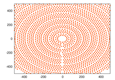
Figure 2: Close look to the first transition lines of the field layout of an optimal 3000 heliostat plant. We can see the transition lines, the number of heliostats in each these transition lines are 2-3-3-4-4-5-… (see text for more details). This optimal layout correspond to the output of the NSPOC code (see Sections 5 and 7 for more details).

After a transition line we have to determine the azimuthal distance again of the next group of heliostats. This is done with the same recursion relation Eq. 3.

$$D_{\alpha}^{a}=D_{\alpha-1}^{a}+e_{\theta}\theta$$ (5)

where the index $a=1,2...$ label groups of heliostats. As was commented before these recursion relations need $D_{0}^{a}$ as an initial condition. These quantities are determined through

$$D_{0}^{a}=(b+1)D_{0}^{a-1}$$ (6)

that essentially allow the azimuthal distance between heliostats in the north to increase/decrease with the radial distance of the group. This last recursion relation needs $D_{0}^{1}$ as an input. This is another optimization parameter completing the 8 parameters needed to optimize a field layout

1. $b:$ Azimuthal distance dependence with the radial distance of the group.

2. $D_{0}^{1}:$ Initial azimuthal distance in the first line of heliostats of the plant.

It is understood that there is a minimal azimuthal distance $D_{\sc min}$ between heliostats that is given by the size of the heliostat plus some arbitrary distance needed for operational purposes.

The only additional information needed is the number of heliostat lines of each group. These are determined by trial and error. Reasonable results are obtained with an increasing sequence like $2-3-3-4-4-5-5-6-6-7-7...$ (see Fig. 2 for an example). The conclusions of this paper are unchanged by the details like how many heliostats each group has, one only needs to fine tune this numbers when looking for the final design of a plant, and this can be easily done in an automated way.

It is important to remark here that the set of variables ([V01–V08]) are compatible with much more conventional field designs. For example having no transition lines is easily achieved by adjusting $\epsilon$ and $\delta$. A constant azimuthal distance between heliostats by setting $b=e_{\theta}=0$, and a constant separation between lines corresponds to the choice $a_{1}=0$. Finally $d_{\theta}=0$ give perfectly circular heliostat lines.

The existence of some of the variables allow more complex designs that we think can improve the plant performance, but this complex design is not imposed. The optimization process will choose between the different options.

Following these rules one generates a general field layout. We chose to fix the number of heliostats of our plant design ($N_{\rm hel}$). In order to choose these heliostats we pick up the ones which contribute with more power to the receiver.

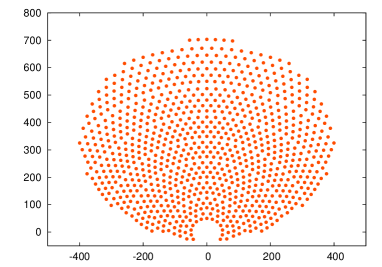
Figure 3: Field layout of an optimal 900 heliostat plant. This optimal layout correspond to the output of the NSPOC code (see Sections 5 and 7 for more details). During the optimization more heliostats are generated but not selected for the final layout due to their worse performance compared to the selected ones (see Fig. 4).

Figure 4: Heliostats not selected for the final layout due to their worse performance. This image shows a subset of all the generated heliostats during the optimization (see text and Fig. 3 for more details.)

In Fig. 3 and Fig. 4 we can see how this procedure works in practice for a 900 heliostat plant. During the optimization process, we generate a field layout with far more than 900 heliostats. To draw the final layout we simply pick the “best” heliostats of the field (those shown in Fig. 3), but more heliostats are generated and rejected due to their worse performance (see Fig. 4).

Note that this rule to select the heliostats does not necessarily impose a circular-like field layout. Simply this layout turns out to be optimal for the problems we are studying here. As an example of a non-circular optimal field, we show in Fig. 5 the field layout of a more complicated plant design with three cavity receivers in the tower (see Crespo and Ramos (2009) for more details). As can be seen in Fig. 5 having three cavity receivers dramatically improves the interception efficiency of some heliostats in the east and west part of the field, making this heliostats to perform better that heliostats that are far in the north. In this case the optimal field layout does not have a circular shape, but clover-like.

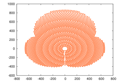
Figure 5: Field layout of a plant with a tower with three receivers. One of them points to the north, and the others at 120^o. As can be seen the presence of two additional receivers increases dramatically the interception efficiency of heliostats at the east and west, making them to contribute with more power to the receiver than other heliostats in the north but more distant. This effect make the optimal field layout to have a clover shape.

2.2 Receiver variables

We can design either a north field plant or a circular plant. In the first case we will consider that the receiver consists on an circular aperture pointing to the north that lets the reflected solar rays to enter. This receiver is characterized by the following variables

1. $h_{T}:$ Tower height $[m]$.

2. $r:$ Aperture radius $[rad]$.

3. $e_{L}:$ Aperture inclination $[rad]$.

In the second case the receiver consists in a cylinder that can absorb radiation coming from all directions. In this case the receiver is characterized by its position and size, parametrized by the following variables

1. $h_{t}:$ Tower height $[m]$.

2. $r:$ Receiver radius $[rad]$.

3. $h_{r}:$ Receiver height $[m]$.

3 Additional input: minimization parameters

To compute the full output of a solar power plant, we need some additional input related with the heliostat characteristics and plant location. These parameters are not treated as variables in the minimization process.

These extra input are seven parameters that define the heliostats characteristics and plant location, plus insolation data from the plant location.

The study on how the plant performance depends on these parameters (what we call parametric analysis) is definitively a very interesting subject that can answer questions like What is the proper heliostat size? How much influence the optical quality of an heliostat the plant performance?, etc… Nevertheless these questions are beyond the scope of the present work and need further investigations (Crespo et al., 2011).

3.1 Heliostat characteristics

An heliostat is characterised by its geometry and its optical properties. All heliostats are assumed to be rectangular, with the focal equal to the slant range and made of spherical facets.

We have a total of four parameters to describe these properties of heliostats. All these parameters can be different for different groups of heliostats (what we call mixed fields):

1. $\sigma_{h}:$ Heliostat optical error.

2. $L_{h}:$ Horizontal length of the heliostat.

3. $L_{v}:$ Vertical length of the heliostat.

3.2 Geographic characteristics

The location and local ground characteristics of the solar power plant are taken into account in the following parameters

1. $\phi:$ Latitude of the plant position.

2. $m_{N}:$ Terrain north-south slope.

3. $m_{W}:$ Terrain east-west slope.

3.3 Insolation and ambiente temperatures

Direct insolation in clear days and ground level temperatures at day hours the 21${}^{\textrm{st}}$ of each month are part of the input data.

Insolation ratios for each month are also input data. This ratio is defined as the relation between the solar energy received in a month and the solar energy received if all days were clear.

4 Performance models

We will not detail all the models used to compute the performance of the power plant, only to say some words and give the appropriate references.

The interception efficiency is computed with an optical model described in (Kiera, 1980a, b).

Atmospheric losses are estimated by the model described in (Biggs and Vittitoe, 1976).

Receiver and cycle efficiency is estimated by taking into account the total input power through the aperture, the aperture size, the aperture inclination and the ambient temperature. This estimation is done by using a polynomial function whose coefficients have been determined by fitting data.

Finally the total daily and yearly energies are computed by integrating the hourly power output. We compute total daily and yearly energies for clean day, and mean cloudy basis.

5 Optimization procedure

Within the framework described in the preceding sections we are in the position to start an optimization procedure. By using the performance models described above we can estimate the total yearly energy output, and with this our optimization citeria, the price of the produced energy, as a function of our eleven design variables ([V01–V11]), seven design parameters ([P01–P07]) and insolation data.

$$E(v_{i};p_{\alpha},I)$$ (7)

where $v_{i}$ ($i=1,\dots,11$) represents the optimization variables, $p_{\alpha}$ ($\alpha=1,\dots,7$) are the design parameters, and $I$ is the insolation data.

One only needs to find the values of $v_{i}$ that makes $E(v_{i};p_{\alpha},I)$ maximum. Being $E(v_{i};p_{\alpha},I)$ a non linear function one should be concerned about the existence of local optima.

To have a full control over the optimization process we have made some tests on typical plant configuration by using several state of the art algorithms. First we will use our own local optimization algorithm (Ramos, 2008), designed with the particularities of solar plant optimization in mind. This is a fast algorithm that find the closest local optimum. Second we will use a mixture of Monte Carlo and conjugate gradient like algorithms coded in the CERN MINUIT library (James and Roos, 1975). Finally we have specifically coded a genetic algorithm (Ramos, 2005) commonly used to solve difficult optimization problems with many local optima.

Algorithms capable of finding global optima are usually much slower than local algorithms. The porpoise of using global searchers is to find out if our preferred local algorithm finds the same optima as global algorithms.

Now we will describe in detail our optimization algorithms.

5.1 NSPOC algorithm

Our preferred local algorithm is a variant of Powell’s algorithm (Powell, 1964).

Starting from an approximate value of the optimal variables $v_{i}^{(0)}$ our algorithm performs a line search along the first direction ($v_{1}$) until a optimum is found with some initial precision $h$. Then the algorithm proceeds with the second direction, and so on, until the 11 variables have been explored. This process needs to be repeated until all the variables are fixed at their optimum for a full cycle. Finally one can increase the precision of the optima position by repeating the process with an increased precision (i.e. setting $h\rightarrow h/2$).

Figure 6: ”Zig-zagging” of the NSPOC algorithm to find the minimum in an example two dimensional function

Following this algorithm we will “zig-zag” until the optima is found (see Fig. 6). One may naively think that this zig-zag results in a very slow convergence, but this turns out not to be the case. Exploring the dimensions one by one instead of approaching the minima along a “direct” route has the advantage that one does not have to fully evaluate the objective function at each step. For example by changing the aperture size or inclination one does not need to recompute the blocking and shadowing effects, or the atmospheric efficiency.

Moreover algorithms that approach the minima along a “direct” route needs additional information from the objective function in order to find the proper direction in which the optima is located. This extra information usually comes from the derivative of the objective function (i.e. the conjugate gradient method (Hestenes and Stiefel, 1952)). We do not have the possibility of computing analytically the derivative of the objective function, and a numerical evaluation of the derivative severely worsen the convergence speed of these algorithms. There also exists methods that tries to avoid the ‘”zig-zagging” without using the derivative (like the original Powell method), but in practice this methods can easily end up searching the optima in a lower dimensional subspace.

In summary, cause the re-evaluation of the objective function is much simpler when only one variable has changed, and because more complicated ingredients need additional knowledge of the objective function to work (like the gradient) our simple variation of Powell’s method turns out to be a fast and robust method for solar power plant optimization.

5.2 MINUIT algorithm

The MINUIT library has been widely used in high energy physics as well as in other fields with literally thousands of papers based in its results. It is considered a robust minimizer. This is the reason we choose to use it here. We refer the reader to the MINUIT reference (James and Roos, 1975) for further details. Here we will only comment that the MINUIT library has several algorithms implemented.

We first use the SEEK optimizer. This is a Monte Carlo search that has potentially the ability to jump over function barriers to find a better global optima. The algorithm includes a metropolis step (Metropolis et al., 1953) which moves to a new position $v_{i}^{(new)}$ from an old one ($v_{i}^{(old)}$) with a probability

$$\mathcal{P}\left(\nu_{i}^{(old)}\rightarrow\nu_{i}^{(new)}\right)\propto\exp\left\{-\frac{E(v_{i}^{(new)};p_{\alpha},I)}{E(v_{i}^{(old)};p_{\alpha},I)}\right\}$$ (8)

We refine this optima search with the use of the MINUIT optimizer MIGRAD, that is consider MINUIT best local optimizer. It is a quasi-Newton method (Davidon, 1991) with inexact line search and a stable metric updating scheme. We decided to use the strategy that make less use of the numerical estimates of the gradient of the objective function at the price of being slower.

Regardless the potential abilities of this combination of MINUIT algorithms it is fair to say that about half of the MINUIT hackers believes that the ability of finding global minima are small in practical situations.

5.3 Genetic algorithm

To be sure that our local optimizer and MINUIT are not falling in local optima, we have also implemented a genetic algorithm  (Ramos, 2005).

Genetic algorithms (Holland, 1975) mimic the process of natural evolution by creating a “population” and implementing natural-inspired mechanisms as crossover, mutation and natural selection to optimize an objective function.

The main ingredients of a genetic algorithm are

1. A population of organisms whose fitness is given by the objective function.

2. A crossover process, by which two members of the population (“parents”) give rise to two different members (“childs”).

3. A mutation process, by which organisms randomly change.

4. A selection process by which the members of the population are chosen for later crossover and/or mutation based in its fitness.

5.3.1 Population

The members of our population have 11 “genes” ($g_{i},\,i=1,\dots,11$) whose values are the 11 variables that code the plant design. In this case these variables are stored simply as a vector of 11 real numbers.

Members of the population have a “fitness” that is given as the value of the objective function evaluated for its genetic content.

$$\textrm{Fitness}=E(g_{i};p_{\alpha},I)$$ (9)

We have repeated the optimization procedure with different population sizes in the range $N_{tot}=30-100$.

5.3.2 Crossover and mutation

The population is paired up, and each pair crosses with a probability $p_{c}$ (typical values in our runs are $p_{c}\approx 0.05$). When a crossover occurs each of the genes of the two members of the population $g_{i}^{(1)}$ and $g_{i}^{(2)}$ produce the offspring with genetic content $g_{i}^{{}^{\prime}(1)}$ and $g_{i}^{{}^{\prime}(2)}$ given by

$$g_{i}^{{}^{\prime}(1)} = r_{i}g_{i}^{(1)}+(1-r_{i})g_{i}^{(2)}$$ (10)

$$g_{i}^{{}^{\prime}(1)} = q_{i}g_{i}^{(1)}+(1-q_{i})g_{i}^{(2)}$$ (11)

where $r_{i},q_{i}$ are samples of a normal distribution $\mathcal{N}(0.5,0.5)$ with mean $1/2$ and standard deviation $1/2$. It is important here to remark that this choice allow interpolation as well as extrapolation between parent’s genetic content, avoiding a fast “false convergence” (see for example Allanach et al. (2004)).

After this process each gene of each member of the population is mutated with a probability $p_{m}$ (typical values in our runs are $p_{m}=0.1$). In this mutation process the gene value is multiplied by $(1+r)$ where $r\sim\mathcal{N}(0,1)$ is a random sample of a standard normal distribution.

5.3.3 Selection

If a member is the product of a crossover or has mutated its fitness (value of the target function) needs to be re-computed.

The “best” $N_{elite}$ of the total population $N_{tot}$ organisms are retained from one generation to the next without change. For the rest we use the well known roulette-wheel selection process (see for example (Goldberg, 1989) and references therein) in which the members of the population are ordered by its fitness and accumulated normalized fitness values are computed (the accumulated fitness value is the sum of the fitness of all the individuals better fitted than itself). After we choose $N_{tot}-N_{elite}$ individuals by drawing uniform random numbers and taken the first individual whose accumulated normalized fitness value is greater than these random samples.

The idea behind this process is that if an organism has a fit that is twice than other organism’s fitness, it is twice as probable for this organism to “survive”.

This members together with the $N_{elite}$ members form the “next generation” that is subject to the same process again. Typically $N_{elite}$ is chosen 5-10.

5.3.4 Stop criteria

The stop criteria is always a subtle matter in a genetic algorithm. We choose to iterate the process a fixed number of generations (in practice around 200), and examine if the fittest organism has changed in the last 20 generations. If this is the case we proceed to iterate for another 200 generations.

In all situations we are sure that when we decide to stop the optimization process, the fitness of the elite ($N_{elite}$) organism has not significantly changed in at most 20 generations.

We also routinely perform tests during the run to ensure that there exists diversity among the organisms to avoid a false fast convergence. The existence of diversity is controlled by computing the variance of each genes in all generations.

6 Impact of the variables in the plant performance

Once one finds the value of the eleven variables that makes the objective function optimal, it is interesting to analyze the properties of this optimum. The basic idea is better understood in a one dimensional case (see Fig. 7).

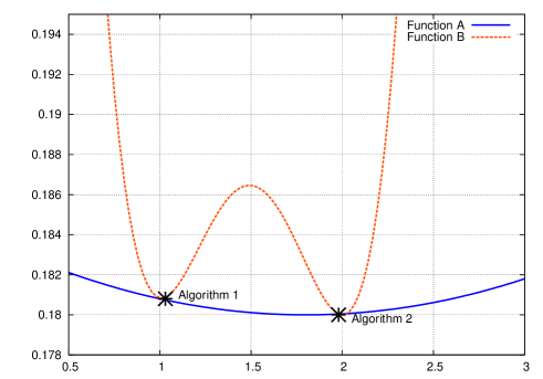
Figure 7: One dimensional example of the minimization of a complex function. Algorithm 1 outputs that the minimum is at $x=1.03$ with a value of the objective function equal to $1.1808$. Algorithm 2 says that the minimum is located at $x=1.98$ with a value of the objective function equal to $1.18001$. These results are compatible with both function types A and B, but the physical interpretation is very different in both cases. A detailed study of the second derivative of the objective function will help us in discerning both cases (see text for more details).

When two algorithms outputs the position of the minimum and the value of the objective function in the minimum they will never give exactly the same answer. When the value of the objective function is very similar, the difference in the position of the minimum can be due to the fact that the minimum is very wide (function A of Fig. 7), or that the function has several local minimum (function B of Fig. 7). These cases can be easily discerned by looking at the second derivative at the minimum. Furthermore, the same analysis also provides information on how the value of different variables affect the plant performance, helping us to detect “irrelevant” variables that we could have included in the design, and to focus in variables that are key for the plant performance. This analysis for the general case of an objective function of several variables will be explained in this section and in the A.

We will assume that the optimal value of the objective function is achieved at $\bar{\nu}_{i}$ and that the value of the objective function at this point is $E(\bar{\nu}_{i};p_{\alpha},I)=\bar{E}$. If we take the value of one variable away from its optimal value by an amount $\sigma(\varepsilon)$ the value of the objective function will increase. But some of the rise in the objective function can be compensated by tuning the other variables. We define the uncertainty of the variable $\nu_{i}$ (and use the symbol $\sigma_{i}(\varepsilon)$) with the condition that the minimum of the objective function with the $i-th$ variable fixed at the value $\nu_{i}=\bar{\nu}_{i}+\sigma_{i}(\varepsilon)$ is equal to $\bar{E}+\varepsilon$ (see Fig. 8).

Figure 8: Contour plot of the function $E(\nu_{i};p_{\alpha},I)$ in the $\nu_{1},\nu_{2}$ plane. The minimum of the function is located at $\nu_{1}=\bar{\nu}_{1}$ and $\nu_{2}=\bar{\nu}_{2}$ (at the center of the ellipse), and the value of the function in this point is $\bar{E}$. The ellipse corresponds to the points that having the values of $\nu_{1}$ and $\nu_{2}$ that correspond to the point in the plane, have a minimum value of the objective function equal to $\bar{E}+\varepsilon$. The size of the ellipse defines the quantities $\sigma_{1}(\varepsilon)$ and $\sigma_{2}(\varepsilon)$. The inclination define the “correlation” between the two variables $\rho_{12}$. This correlation can also be estimated from the difference between $\sigma_{\rm inner}$ and $\sigma(\varepsilon)$.

If $\varepsilon$ is chosen small, a large value of $\sigma_{a}(\varepsilon)$ means that the variable $\nu_{a}$ plays no role in the plant performance. It does not matter the value we choose for $\nu_{a}$ the objective function will not deviate from its optimal value. On the other hand if $\sigma_{a}(\varepsilon)$ is small this means that any departure of $\nu_{a}$ from its optimal value will severely worsen the plant performance. Note that this uncertainty is an estimate of how wide the minimum is. In our one dimensional example of Fig. 7 the uncertainty of the variable $x$ is about 0.7 for the function A and 0.08 for the function B using a value of $\varepsilon=0.001$.

When missing the minimum for a variable $i$ can be compensated by tuning the variable $j$ we say that the variables $i$ and $j$ are correlated. They share part of the information of a plant design. For example the tower height and the aperture inclination must be correlated, since we need to adjust the aperture inclination to correct an error in the tower height. We can say that both variables “share” the information that the aperture need to look directly to the field in order to increase the interception efficiency. This correlation can be mathematically expressed by the correlation coefficient between the two variables $\rho_{ij}$, a real number between -1 and 1 that measures the difference between the quantity $\sigma_{i}(\varepsilon)$ and its would-be value if the variable $j$ would have stayed fixed at its minimum value $\bar{\nu}_{J}$ (the quantity $\sigma_{\rm inner}$ in Fig. 8).

A value of $\rho_{ij}$ close to zero means that the variables $\nu_{i}$ and $\nu_{j}$ encode different information of the plant design. On the other hand if $\rho_{ij}$ is close to its extreme values $\rho_{ij}\approx\pm 1$, both variables $\nu_{i}$ and $\nu_{j}$ encode the same information, since a non optimal value of one of them can always be compensated by choosing the other appropriately.

On one hand if a plant design variable has a very large uncertainty this variable can be dropped from the plant design, since it plays no role in the plant performance. On the other hand, ideal plant design variables should be as uncorrelated as possible, since otherwise the optimization algorithm will be looking for an optimal value of a function with an almost flat direction.

We are interested in computing the quantities $\sigma_{i}(\varepsilon)$ and the correlation matrix $\rho_{ij}$. As it is shown in the A, when $\varepsilon$ is small, these quantities can be estimated by computing the Hessian of the objective function evaluated at the minimum

$$H_{ij}=\left.\frac{\partial^{2}E(\nu_{i};p_{\alpha},I)}{\partial\nu_{i}\partial\nu_{j}}\right|_{\nu=\bar{\nu}}.$$ (12)

Being concise, the quantities $\sigma_{i}(\varepsilon)$ are given by the diagonal elements of the inverse of the Hessian

$$\sigma_{i}^{2}(\varepsilon)=(H^{-1})_{ii}\,\varepsilon,$$ (13)

and the correlation coefficients are given by the normalized non diagonal elements of the inverse hessian

$$\rho_{ij}=\frac{(H^{-1})_{ij}}{\sqrt{(H^{-1})_{ii}(H^{-1})_{jj}}}.$$ (14)

We emphasize here that this expressions are accurate only in the case that $\varepsilon$ is small enough so that all the $\sigma_{i}(\varepsilon)$ are small. For practical purposes we can only consider the resulting $\sigma_{i}(\varepsilon)$ an estimate of the real uncertainties, but this information is more than enough to obtain a qualitative understanding of how the different design variables impact the plant performance and to interpret the result of the optimization that different algorithms produce.

The strategy that we follow once the optimal value of the design variables is found is to compute numerically the Hessian matrix, and then invert it. To compute the numerical first and second derivatives we use standard finite differences expressions (we drop the non variable arguments of $E$ for clarity):

$$\frac{\partial E(\nu_{i})}{\partial\nu_{k}} = \lim_{h\rightarrow 0}\frac{E(\nu_{i}+h_{k}\hat{k})-E(\nu_{i}-h_{k}\hat{k})}{2h}$$ (15)

$$\frac{\partial^{2}E(\nu_{i})}{\partial^{2}\nu_{k}} = \lim_{h\rightarrow 0}\frac{E(\nu_{i}+h_{k}\hat{k})-2E(\nu_{i})+E(\nu_{i}-h_{k}\hat{k})}{h^{2}}$$ (16)

$$\frac{\partial^{2}E(\nu_{i})}{\partial\nu_{k}\partial\nu_{j}} = \lim_{h_{l}\rightarrow 0}\frac{1}{4h_{k}h_{j}}\left\{E(\nu_{i}+h_{k}\hat{k}+h_{j}\hat{j})\right.$$ (17)

$$- E(\nu_{i}+h_{k}\hat{k}-h_{j}\hat{j})$$

$$- E(\nu_{i}-h_{k}\hat{k}+h_{j}\hat{j})$$

$$+ \left.E(\nu_{i}-h_{k}\hat{k}+h_{j}\hat{j})\right\}$$

where $\hat{i}$ represents the unit vector in the direction of the variable $\nu_{i}$.

Choosing an appropriate step size (the values for $h_{i}$ in the previous formulas) is crucial to compute derivatives numerically. This is a well known problem: numerical differentiation is an ill defined problem for finite precision arithmetic.

We have chosen a step size $h_{i}$ for each direction that meets the following two criteria:

1. The numerical computation of the first derivative gives a very small result.

2. The numerical computation of the second derivative gives approximately the same result if we vary the step by a 10-20%.

The first condition ensures that we are not having rounding errors (being at the minimum means that the first derivative should be zero). The second condition ensures that the computation of the second derivatives is stable.

7 Results

Following the steps described in the previous sections we will present some results about the optimal field design of some typical solar power plants.

For the case of a cavity receiver we will analyze the case of a 900 heliostat power plant. This plant produces aound $15$ MWe. We will label this plant as N900.

For the case of the cylindrical receiver we will analyze the case of a 3000 heliostat field. This circular filed layout produces around $50$ MWe. We will label this plant C3000.

In both cases the optimization criteria consist in finding the cheapest price for the generated power.

7.1 Algorithm analysis

First we will focus in the N900 plant. In Tab. 1 we can see the result of the optimization procedure with each of the algorithms. As can be seen the three algorithm give a similar result for the value of the objective function at the minimum (quantity $\overline{E}$). Nevertheless, this optimal value is achieved with different values of some of the variables. The value of $a_{0}$ is 5.4 for the minimum found by the NSPOC algorithm and $2.3$ for the Genetic one. Since the value of the objective function is almost the same. This may induce to think that the objective function has several almost degenerate local minimums.

	NSPOC	Genetic	MINUIT	$\sigma(\varepsilon=0.001)$
$\overline{E}$	0.18092	0.18113	0.18311	N/A
$a_{0}$	5.4	2.3	3.5	2.8
$a_{1}\times 10^{2}$	3.15	3.78	3.37	0.55
$d_{\theta}$	-9.5	-1.9	-5.4	8.1
$e_{\theta}$	-0.05	-0.78	-0.01	0.66
$\epsilon$	0.88	0.24	1.8	1.1
$\delta$	0.169	0.024	0.015	0.097
$b\times 10^{3}$	54.2	32.8	29.6	24.0
$D_{0}^{0}$	16.8	19.5	19.1	2.5
$h_{T}$	120.	117.	123.	12.
$r$	10.78	10.74	10.85	0.99
$e_{L}$	28.6	26.5	38.1	9.3

Table 1: Comparison of the three algorithms for the N900 plant. The second, third and fourth column shows the results for the NSPOC, the Genetic and the MINUIT algorithm respectively. Finally the last column quote the values of $\sigma(\varepsilon)$ for a change in the function of $\varepsilon=0.001$. The first row show the value of the function at the minima. Subsequent rows show the value of each of the design variables. . The following lines shows the value of different variables at the minima for each algorithm.

But nothing could be more wrong. As our minimum analysis shows all these values corresponds (approximately) to one and the same minimum. But this minimum is very wide in some of the directions. This can be seen by computing the uncertainties needed to change the objective function value in an amount $\varepsilon$ for each of the directions. We will choose $\varepsilon=0.001$ as an estimate of the difference of the optimum value obtained by different algorithms. Clearly this small change of the objective function does not change the plant properties, since in the plant evaluation one uses approximations that lead to an estimate of the plant performance that is accurate with less precision than this value of $0.001$.

As can be seen in Tab.1 the variables that show a strong discrepancy between the results of different algorithms corresponds to directions in the objective function in which the minimum is very wide. For the case of $a_{0}$ the associated uncertainty is 2.8, meaning that the values 5.42 and 2.27 that different algorithms find correspond to the same optimum. This confirms that all algorithms are finding the same minimum, but that in this minimum the objective function has a very mild dependence with some variables. Variables that are crucial for the plant design are the ones that have a small associated uncertainty, like for example $a_{1}$ or $r$. For this variables we can see that all algorithms find approximately the same value of the objective function.

In one sentence, the discrepancy between the value of the value of the variables at the minimum obtained with different algorithms is nicely explained once ones analyzes how strong is the dependence of the objective function at the minimum with respect to different variables. One can conclude that all the algorithms are finding the same basic plant design.

Also we have checked that the correlations between parameters are not large. The largest correlation turns out to be between variables $b_{0}$ and $b_{1}$, and amounts to 0.91. Note that precisely these are the variables with a large uncertainty. Variables with small associated uncertainties have usually small correlations. For example in the case of $r$ and $a_{1}$ the correlation amounts to $-0.08$.

The correlation matrix also seem to pick up important information of the plant design. For example the tower height $h_{T}$ is positively correlated with the aperture inclination $e_{T}$ (the correlation amounts to $0.1$), indicating that if ones makes the tower higher one needs to incline more the aperture.

	NSPOC	Genetic	MINUIT	$\sigma(\varepsilon=0.001)$
$\overline{E}$	0.17022	0.16981	0.17023	N/A
$a_{0}$	0.97	0.27	0.25	0.26
$a_{1}\times 10^{2}$	3.40	3.52	3.29	0.35
$d_{\theta}$	-1.4	-2.8	-5.3	1.9
$e_{\theta}$	-0.5	0.0	1.8	1.5
$\epsilon$	0.29	0.37	0.16	0.55
$\delta$	0.109	0.081	0.134	0.039
$b\times 10^{3}$	40.	60.	47.	13.
$D_{0}^{0}$	17.8	15.3	15.1	1.9
$h_{T}$	145.	147.	152.	13.
$r$	8.58	8.66	8.57	0.96
$h_{r}$	8.14	8.15	8.17	0.96

Table 2: Comparison of the three algorithms for the C3000 plant. The second, third and fourth column shows the results for the NSPOC, the Genetic and the MINUIT algorithm respectively. Finally the last column quote the values of $\sigma(\varepsilon)$ for a change in the function of $\varepsilon=0.001$. The first row show the value of the function at the minimum ($\overline{E}$). Subsequent rows show the value of each of the design variables. The following lines shows the value of different variables at the minimum for each algorithm.

In Tab.2 we can see the same information for the case of the C3000 plant. As we can see the conclusions are roughly the same. The three algorithms seem to find the same design as can be seen by comparing the values of the variables at the minimum found by different algorithms with their respective uncertainties.

Comparing Tab. 1 and Tab. 2 we observe that in general the uncertainties are smaller for the C3000 plant. This means that for the design of bigger plants variables need an accurate value if we want to obtain a high performance. The design of solar power plants become more involved and difficult when the size of the power plant increases. This conclusion seem intuitively correct, since there are some variables (ej. $d_{\theta}$ that “compress” the field layout in the south) that seem to be crucial only for big circular plant designs, and more or less irrelevant for the design of small power plants.

7.2 Performance analysis

A summary of the performance of the different algorithms is presented in Tab. 3.

PLANT	Algorithm	Calls	Time $[s]$	Time $[a.u.]$
N900	NSPOC	1270	17280	1.00
	MINUIT	3737	86450	5.00
	Genetic	2381	40539	2.35
C3000	NSPOC	1872	41460	1.00
	MINUIT	4599	102699	2.47
	Genetic	10398	254829	6.14

Table 3: Running times of the different algorithms in our prototype plants. The first three columns corresponds to the 900 heliostat north field plant N900, and the last three columns to the 3000 heliostat cylindrical receiver plant C3000. The table shows the number of calls to the plant evaluation function as well as the time of the run, both in seconds and relative to the running time of the NSPOC algorithm. As the reader can see, it took for the global algorithms (both MINUIT and Genetic) between 2.5 and 5 times more time to find the optimum plant design than the time used by NSPOC for the case of the plant N900. In the case of the plant C3000 the case is worse (between 4 and 7 times more time).

The NSPOC algorithm is always faster than the global optimizers MINUIT and Genetic. In the case of the plant N900, MINUIT uses 5 times more time to achieve the optimum, while Genetic uses 2.35 more time than NSPOC. This difference is similar for the case of the C3000 plant.

The two global optimizers that we have used are stochastic in nature, thus this running times should not be treated as exact numbers, but they are representative, and the conclusion is always the same: the NSPOC algorithm outperforms the global optimizers while giving the same results.

As we have said, the NSPOC code only re-compute the “needed” pieces of the objective function. For example blocking and shadowing effects are not computed when we perform a line search in the direction of the aperture size. This approach seems to be very successful for the case of the N900 plant. On average each function call takes between a 25% and a 50% less time for the NSPOC algorithm than for the others. In the more involved case of the C3000 plant the NSPOC function calls still are faster, but with a large margin.

8 Conclusions and perspectives

We have presented and analyzed a method to design solar power plants. Based in the field layout done within the German-Spanish GAST project (1982-86) in the company INTERATOM, we have proposed a method to design solar power plants. This method reduces the plant design to the value of 11 variables that determine the field layout, tower and receiver characteristics. The problem of finding optimal plant designs is reduced to the numerical problem of optimizing a non linear function.

Due to the non linear nature of the target function and the high computational costs of evaluating plant performances, it is crucial to find a robust and fast algorithm to perform plant designs. Fast algorithms to optimize functions of several variables are local in nature: they find a local optima of the target function, but give no information on the possible existence of other global optima. On the other hand global optimizers are much more computationally expensive and their coding is far more involved.

In this work we have tackled the optimization problem with different algorithms, both local and global. We have shown that in all the cases our local NSPOC algorithm give the same results as other more complex optimizers with significantly less computing effort.

The design variables that we have choosen have enough flexibility to provide solar plant layouts with very high performance for a broad range of sizes: from small $10$ MWe plants to big $200$ MWe plants. With our choice of variables we find that our local optimizer outperforms global optimizers.

In analyzing the result of different algorithms we have also developed an interesting method to get information on how different variables affect the performance of an optimal design. The method is based in analyzing the Hessian of the objective function at its optimum value, and gives us an estimate of how much the departure of a variable from its optimal value affects the plant performance. We have observed that circular-like big plants need a more accurate tuning of the variables in order to achieve an optimal performance.

This information can be used to speed up the optimization process. It turns out to be convenient to first tune variables that are crucial for the optimal design, and only after worry about variables that have a mild impact in the plant performance. Our NSPOC algorithm partially profit from this information to speed up the convergence to the optimum.

Moreover, this method of evaluating the impact of design variables in the plant performance is key to the study of the improvement of plant designs. Any new proposed design should include a similar analysis to detect superfluous variables in the design and determine what are the key ingredients of the new design.

This works provide the tools to address very interesting problems, what we call parametric analysis, in which the efficiency of the solar power plant can be studied as a function of plant design parameters. Questions like Does a terrain with slope improve the plant efficiency? How much does the heliostat aspect ratio affect the plant efficiency? Can we build cheaper plants by using cheaper heliostats without losing efficiency? Some of these questions are currently under study by the authors, and preliminary results were presented in the solarPACES 2011 conference (Crespo et al., 2011).

We have also provided the basis to analyze more complex plant designs. An example that we consider very interesting are multi-tower layouts, in which a solar power plant is built with several towers, and heliostats choose which tower they aim based on performance (some results were already presented in the 2009 solarPACES conference (Crespo and Ramos, 2009)), but there are many more possibilities like multi-cavity receivers, or properly addressing the scalability problem in solar power plant designs: How can we build small plants that can later be enlarged without loosing performance? Some of this questions and others within the framework presented here are currently being studied.

Appendix A Computation of uncertainties and correlations.

The techniques described in this appendix are typical in statistical description of data. In this context the function that one wants to optimize is the quadratic deviation between data and predictions of a model (usually called $\chi^{2}$). Thus any interested reader can consult any standard book on statistics for a more detailed proof of the expressions developed here. We will assume that we are minimizing an objective function. The expressions remain basically unchanged for the case of the maximization of a function if one changes the sign of $M$, $(M^{-1})$ and the Hessian in the expressions that follow.

We will start assuming that our objective function of $n$ variables ($x_{i},i=1\dots,n$) is quadratic with a minimum located at $x_{i}=\bar{x}_{i}$. The most general function with these characteristics can be written as

$$f(x)=f_{0}+\sum_{ij}(x_{i}-\bar{x}_{i})M_{ij}(x_{j}-\bar{x}_{j})$$ (18)

where $f_{0}$ is the value of the function at the minimum and $M_{ij}$ is a symmetric positive definite matrix. To obtain $\sigma_{a}(\varepsilon)$ we will define a new function $g(x_{k})$ ($k\neq a$) of $n-1$ variables (all but the $a-th$) equal to the value of the original function with $x_{a}$ fixed at $x_{a}=\bar{x}_{a}+\sigma_{a}(\varepsilon)$.

$$g(x_{k}) = f\left(x_{k},x_{a}=\bar{x}_{a}+\sigma_{a}(\varepsilon)\right)$$ (19)

$$= f_{0}+\sum_{i,j\neq a}(x_{i}-\bar{x}_{i})M_{ij}(x_{j}-\bar{x}_{j})$$

$$+ 2\sum_{i\neq a}(x_{i}-\bar{x}_{i})M_{ia}\sigma_{a}(\varepsilon)+M_{aa}\sigma_{a}^{2}(\varepsilon).$$

Taking the gradient of $g(x_{k})$ and equating it to zero we obtain the position of the minimum value of the objective function at fixed $x_{a}=\bar{x}_{a}+\sigma_{a}(\varepsilon)$.

$$\frac{\partial g}{\partial x_{k}}=0\Longrightarrow x_{k}^{*}=\sum_{i\neq a}\left(m^{-1}\right)_{ki}M_{ia}\sigma_{a}(\varepsilon)$$ (20)

where $m$ is the minor matrix that corresponds to the element $(a,a)$ (this is the matrix that results from $M$ cutting down the $a^{th}$ column and rows), and $m^{-1}$ is its inverse. The value of the objective function at this point is given by

$$g(x_{k}^{*}) = f\left(x_{k}^{*},x_{a}=\bar{x}_{a}+\sigma_{a}(\varepsilon)\right)$$ (21)

$$= f_{0}+\left[M_{aa}-\sum_{i,j\neq a}M_{ai}\left(m^{-1}\right)_{ij}M_{ja}\right]\sigma_{a}^{2}(\varepsilon)$$

the quantity between brackets can easily be recognised as $1/\left(M^{-1}\right)_{aa}$ (the inverse of the diagonal entry of the original matrix $M$). The condition that determines $\sigma_{a}(\varepsilon)$ is that the increase in the function respect the value at the minimum should be $\varepsilon$. So the quantity $\sigma_{a}(\varepsilon)$ is given by

$$\sigma_{a}^{2}(\varepsilon)={\left(M^{-1}\right)_{aa}}\,{\varepsilon}.$$ (22)

If we define $\sigma_{{\rm inner}}(\varepsilon)$ as the would-be $\sigma_{a}(\varepsilon)$ without tuning the variable $j$, it is clear that a comparison between $\sigma_{a}(\varepsilon)$ and $\sigma_{{\rm inner}}(\varepsilon)$ would give us information about the correlation between variables $i$ and $j$. If we define the correlation coefficient between variables $i$ and $j$ by the equation

$$\rho_{ij}=\frac{(M^{-1})_{ij}}{\sqrt{(M^{-1})_{ii}(M^{-1})_{jj}}}$$ (23)

we can easily check that $\sigma_{{\rm inner}}(\varepsilon)$ and $\sigma_{a}(\varepsilon)$ are related by

$$\sigma^{2}_{\rm inner}=(1-\rho^{2}_{ij})\sigma^{2}_{j}(\varepsilon).$$ (24)

Note that in the case $\rho_{ij}=0$ the two quantities are equal.

In the case that the objective function is not quadratic, we can use Taylor theorem. Close enough to the minimum any function is well approximated by a quadratic function. This means that for a general function the role of $M_{ij}$ is played by the Hessian evaluated at the minimum

$$M_{ij}=\left.\frac{\partial^{2}f(x_{i})}{\partial x_{i}\partial x_{j}}\right|_{x=\bar{x}}+\mathcal{O}(x-\bar{x})^{2}.$$ (25)

It is worth noting that this approximation will fail if $\sigma_{a}(\varepsilon)$ is large. In order to ensure that this does not happen one need to keep $\varepsilon$ sufficiently small.

References

- Allanach et al. (2004) Allanach, B., Grellscheid, D., Quevedo, F., 2004. Genetic algorithms and experimental discrimination of SUSY models. JHEP 0407, 069. hep-ph/0406277.
- Biggs and Vittitoe (1976) Biggs, F., Vittitoe, C.N., 1976. The HELIOS model for the optical behaviour of reflecting solar concentrations. Sandia laboratories SAND76-0347, 121.
- Crespo and Ramos (2009) Crespo, L., Ramos, F., 2009. NSPOC: A new powerful tool for heliostat field layout and receiver geometry optimizations, in: Proceedings of the SolarPACES 2009 conference, Berlin.
- Crespo et al. (2011) Crespo, L., Ramos, F., Martinez, F., 2011. Questions and answers on solar central receiver plant design by NSPOC, in: Proceedings of the SolarPACES 2011 conference, Granada.
- Davidon (1991) Davidon, W.C., 1991. Variable metric method for minimization. SIAM Journal on Optimization 1, 1–17.
- Goldberg (1989) Goldberg, D.E., 1989. Genetic Algorithms in Search, Optimization, and Machine Learning. Addison-Wesley, New York.
- Hestenes and Stiefel (1952) Hestenes, M.R., Stiefel, E., 1952. Methods of Conjugate Gradients for Solving Linear Systems. Journal of Research of the National Bureau of Standards 49.
- Holland (1975) Holland, J.H., 1975. Adaptation in Natural and Artificial Systems. University of Michigan Press.
- James and Roos (1975) James, F., Roos, M., 1975. Minuit: A System for Function Minimization and Analysis of the Parameter Errors and Correlations. Comput. Phys. Commun. 10, 343–367.
- Kiera (1980a) Kiera, M., 1980a. Abbildung der sonne auf die apertur eines sonnenkrftwerkes. GAST project imb-BT-a20000-12.
- Kiera (1980b) Kiera, M., 1980b. Feldoptimierung bei variationen de parameters. GAST project imb-BT-320000-05.
- Metropolis et al. (1953) Metropolis, N., Rosenbluth, A., Rosenbluth, M., Teller, A., Teller, E., 1953. Equations of State Calculations by Fast Computing Machines. Journal of Chemical Physics 21 (6), 1087–1092.
- Powell (1964) Powell, M., 1964. An efficient method for finding the minimum of a function of several variables without calculating derivatives. Computer Journal 7, 155–162.
- Ramos (2005) Ramos, A., 2005. A FORTRAN genetic algorithm library. https://github.com/ramos/libga.
- Ramos (2008) Ramos, F., 2008. NSPOC: Nevada solar plant optimization code. http://www.nspoc.com.