Network Sampling Based on NN Representatives

Abstract

The amount of large-scale real data around us increase in size very quickly and so does the necessity to reduce its size by obtaining a representative sample. Such sample allows us to use a great variety of analytical methods, whose direct application on original data would be infeasible. There are many methods used for different purposes and with different results. In this paper we outline a simple and straightforward approach based on analyzing the nearest neighbors (NN) that is generally applicable. This feature is illustrated on experiments with weighted networks and vector data. The properties of the representative sample show that the presented approach maintains very well internal data structures (e.g. clusters and density). Key technical parameters of the approach is low complexity and high scalability. This allows the application of this approach to the area of big data.

- Information filtering

1 Introduction

In the area of big data, sampling may help facilitate knowledge discovery from large-scale datasets. Using analytical methods it is possible to find patterns and regularities in a sample which is significanly smaller than the original dataset. To be able to validate observed patterns on the original data, it is necessary to have a representative sample which retains certain statistical properties.
In the area of complex networks those are topological properties of the network, i.e. degree, clustering coefficient, and eigenvalues, which are used to evaluate the ’goodness’ of the sample. Those properties are traditionally defined primarily for unweighted networks, as in [8]. In the area of large datasets with vector data it is usually the assessment of the extent to which the sample maintains clusters and their density [5, 11]. Generally, the approaches can be divided into two groups; unbiased (uniform random sampling) and biased. Approach described in this paper is one of the biased methods and is based on the selection of representatives, i.e. objects that in their surroundings play a more important role than others. In the case of networks it means the selection of nodes into a sample after the assessment of their representativeness. Simply stated, by representativeness we understand the extent to which a node is the nearest neighbor of other nodes in the network.
Our method has five important aspects that will be subsequently described in the paper. The first is determinism. A representative sample is uniquely determined by the parameters specified in the method. The second aspect is based on the fact that a key feature used to assess the representativeness is the similarity. The consequence is that the method is applicable to the weighted networks in which the weight of the edges can be understood as the similarity of the nodes. If we accept the non-symmetry of similarity, then the third aspect is the applicability of the method on directed weighted networks. However, in this paper we work with the assumption that similarity is symmetric. The assumption of symmetry leads to the fourth aspect which is locality. A representative sample can be extracted from certain parts of the network (e.g. around the selected node) without the need to analyze the entire network. The method works only with the surroundings of the examined nodes. The locally extracted sample is then a subset of a representative sample of the entire network. That implies the scalability of the presented algorithm. The last, fifth aspect, is the applicability of the approach on other than the network data. If we have data records represented by points (vectors) in an n-dimensional space, then the distance between the points can be interpreted as dissimilarity. By converting dissimilarity into similarity, the problem of obtaining a sample from an n-dimensional dataset in the vector space can be modified to the problem of finding a sample of the network. This aspect will be analyzed in more detail in Section 4.
We illustrate the usage of our method on experiments with small network and 2-dimensional dataset as well as on two large real world datasets. The first is the weighted co-authorship network with more than 300,000 nodes based on the DBLP database. The second is a list of all address points in the Czech Republic, 2.7 million points in total.

2 Related work

Sampling has already been applied to various types of data in many areas. For large n-dimensional datasets sampling methods have been developed in order optimize data mining tasks [3, 5, 10, 11], such as clustering or outlier detection.
In the area of networks, sampling goals range from speeding up simulations [6] to refined visualization [12]. The evaluation of sampling algorithms is related to the sampling goals [1, 13]. In the area of large-scale social networks a work of Leskovec et al. [8] compared state-of-the-art sampling algorithms and defined representative subgraph sampling based on several topological properties. In [2] proposed Metropolis subgraph sampling, where the measuring of graph properties is included as a sampling step. On sampling community structure focused in [9], where the goal was to preserve and infer community affiliation of nodes in the network.
All of the above mentioned methods produce a random sample from an original dataset, while in our approach sampling is deterministic. Therefore, the resulting representative sample is determined by the configuration of the algorithm.

3 Proposed method

In this section we define the key concepts precisely and propose a general sampling approach based on representatives.

3.1 Notations and Definitions

Let $\mathbf{D}$ be the dataset. For a dataset consisting of vector data, sample $\mathbf{S}$ is a subset of those vectors. For a network or graph $G=(V,E)$, $\mathbf{S}$ is a sample of nodes where $S\subset V$.

Object is a basic entity from a dataset $D$.

Similarity is a relationship between two objects. It is a function $s:\mathbf{D}\times\mathbf{D}\rightarrow\mathbb{R}_{0}^{+}$.

Proximity is a similarity greater than a specific threshold. It is a function $p:\mathbf{D}\times\mathbf{D}\rightarrow\{0,1\}$. Object $o$ is close to object $o^{\prime}$ if $p(o,o^{\prime})=1$.

Large similarity is equivalent to a small distance.

Neighbor is an object close to an examined object.

Neighborhood is a set of all neighbors of an examined object, $\varepsilon(o)=\{o^{\prime}\in D:p(o,o^{\prime})=1\}$.

Nearest neighbor is a neighbor that is closest to an examined object. An object can have more than one nearest neighbor.

The importance of an object is determined by its relationship to its surroundings. Generally, significant is the number of neighborhoods in which the object is present and how many times it is the nearest neighbor.

Proximity degree is the number of objects that are neighbors of an examined object and also the number of neighborhoods that contain the examined object. It is a function $d:\mathbf{D}\rightarrow\mathbb{N}_{0}$.

Proximity rank is the number of objects to which an examined object is a nearest neighbor. It is a function $k:\mathbf{D}\rightarrow\mathbb{N}_{0}$.

Representativeness is the property that expresses the extent to which the examined object can represent other objects in the dataset. Representativeness should be based mainly on the proximity rank, but may also reflect the proximity degree. It is a function $r:\mathbf{D}\rightarrow\mathbb{R}_{0}^{+}$.

Representative is an object whose representativeness is equal to or greater than a constant (or otherwise defined) threshold. A function $f:\mathbf{D}\rightarrow\{0,1\}$ describes that objects $o$ is a representative of a set $D$.

On the basis of the representatives, it is possible to define a sample of objects that represent the entire dataset.

Representative sample is a set of all representatives of a dataset. It is a set $S=\{o\in D:f(o)=1\}$ which is defined by $(\mathbf{D},s,p,r,f)$.

Remark 1.

The functions of similarity and proximity do not have to be symmetric.

3.2 Sampling algorithm

Our aproach to obtaining a representative sample of a dataset is inpired by the method of finding nearest neighbors. The algorithm is based on the idea, that objects, which are the nearest neighbors of other objects, are the important ones in a dataset. It is a local oriented algorithm, which reduces the given dataset to its sample.

input : dataset $D$

output : sample $S$

choose a function for $similarity$, $proximity$, $representativeness$ and $representative$

foreach object $o\in D$ do

       find neighborhood $\varepsilon(o)$ and a set of nearest neighbors $NN(o)$

       foreach object $x\in\varepsilon(o)$ do

             increase its $proximity$ $degree$

       end foreach

      foreach object $y\in NN(o)$ do

             increase its $proximity$ $rank$

       end foreach

      

end foreach

foreach object $o\in D$ do

       if $o$ is a $representative$ then

             add $o$ to $S$

            

       endif

      

end foreach

Algorithm 1 Sampling algorithm

4 Experimental evaluation

4.1 Datasets and setup

We tested our algorithm on the 4 following datasets. Two of them representing weighted networks (Miserables [4] and DBLP, a co-authorship network). And other two representing a 2-dimensional data (Birch3 [14], synthetic data with 100,000 vectors and Czech republic map, a set of all address points in the Czech Republic). For datasets characteristics see Table 1, where n = dataset size, e = number of edges, dim = dataset dimensionality.

Table 1: Characteristics of Datasets

dataset	n	e	dim	type
Miserables	77	254	-	weighted network
DBLP	318,971	786,384	-	weighted network
Birch3	100,000	-	2	vector data
Czech map	2,740,903	-	2	vector data

In all experiments we use the function of representativeness $r(o)=\frac{k(o)}{\log_{x}d\left(o\right)}$. For $d(o)=0$ we define $r(o)=0$. For $d(o)=1$ we define $r(o)=k(o)$. Resulting size of the sample depends on two parameters. The first is the logarithm base $x$, the second is the function $f$ that is used to define representativeness. For our experiments we chose $f:r(o)\geq 1$. We must also define the functions for the similarity, proximity, which is done separately in the experiments. We were looking for representative samples of different sizes for each dataset. For every obtained sample, we give the summary of its size as a percentage against the original dataset, the base of the logarithm in function $r$ and some other characteristics.

4.2 Experiment 1 - Weighted Networks

We choose the weight of an edge as a similarity function. The proximity is defined as follows; close to an examined node are all of its adjacent nodes.

First dataset is a co-appearance network of characters in the novel Les Miserables in which the edges have weights from 1 to 31, see Figure 5. Table 2 summarizes the results of the sampling. For the resulting sample networks see Figures 5-5.

Table 2: Les Miserables Dataset Sampling

Log base	Nodes	Edges	Nodes %	Edges %
-	77	254	100	100
3	31	67	40	26
2	22	27	29	11
1.8	10	12	13	5

Second dataset is a co-authorship network contructed from a DBLP dataset. Data were downloaded in april 2013 and preprocessed for the Forcoa.NET system. Edge weights are based on network evolution and forgetting function that takes into account the frequency and regularity of publishing, for details see [7]. After the preprocessing a total of 318,971 nodes (active authors) and 786,384 edges (with a maximum weight of 433.459) remained in the network. Table 3 summarizes the results of the sampling. Figure 5 captures co-authors of Christos Faloutsos as a weighted network. For the resulting samples from this part of network see Figures 5-5.

Table 3: DBLP Dataset Sampling

Log base	Nodes	Edges	Nodes %	Edges %
-	318,971	786,384	100	100
2	180,694	404,624	57	51
1.5	112,885	213,758	35	27
1.3	37,287	67,129	12	9

How some of the topological properties of sampled networks are maintained is depicted on Figure 1. The cumulative degree and edge weight distributions clearly copy the distributions of the original network.

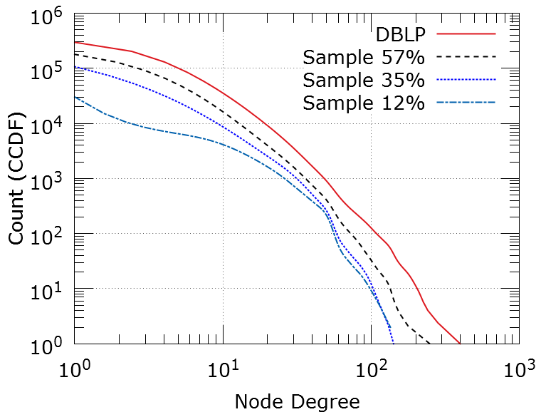
(a)

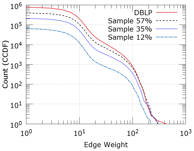
(b)

Figure 1: DBLP sample metrics

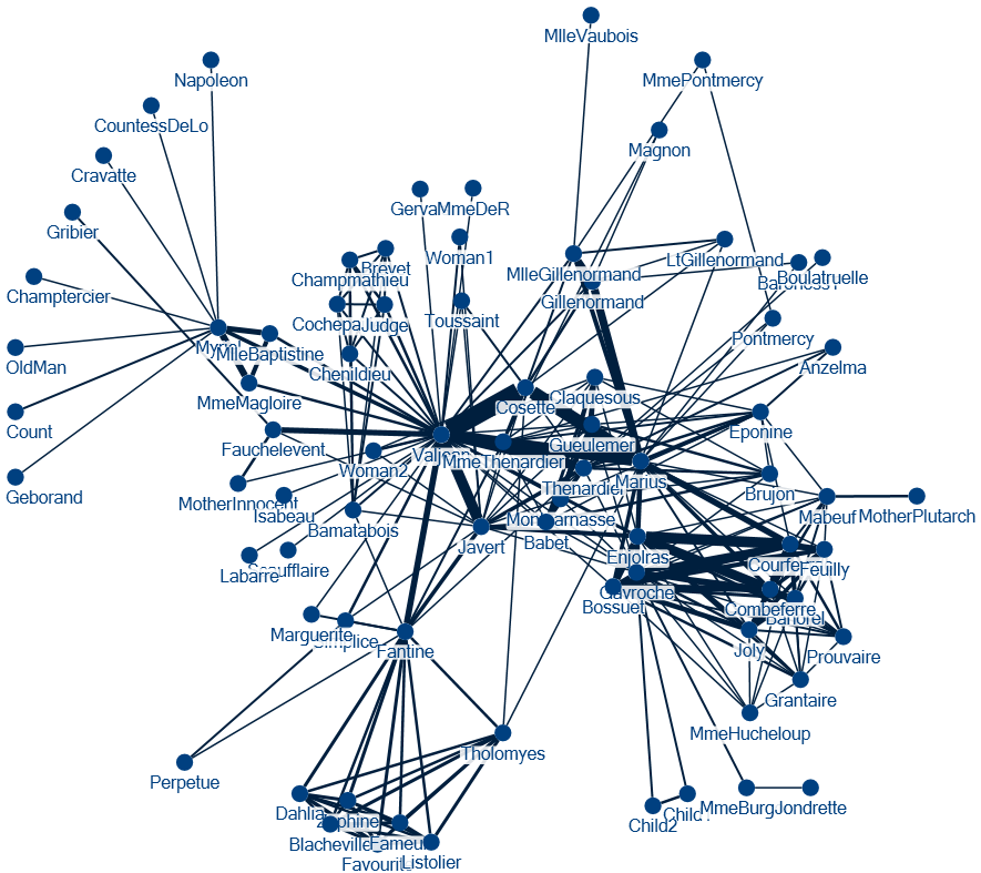
Figure 2: Miserables

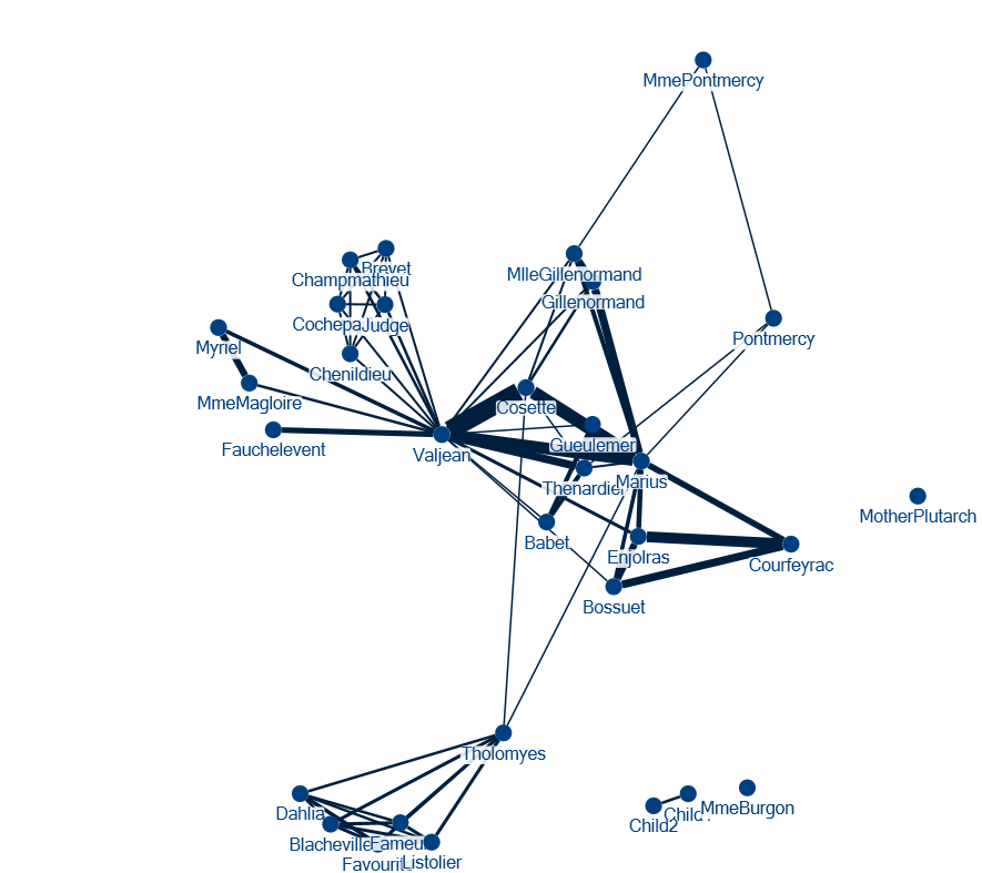
Figure 3: Sample 40%

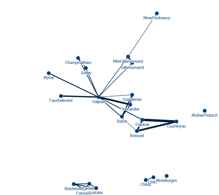
Figure 4: Sample 29%

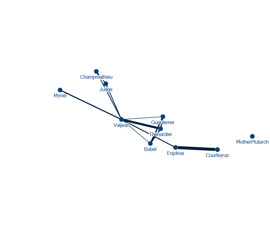
Figure 5: Sample 13%

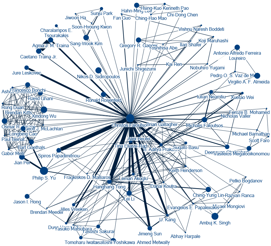
Figure 6: DBLP Faloutsos

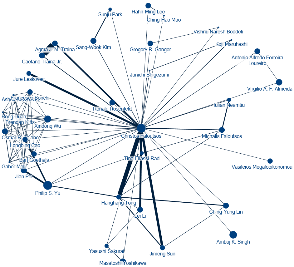
Figure 7: Sample 57%

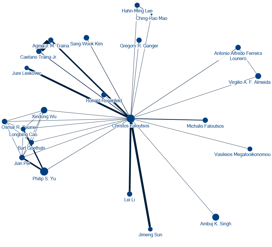
Figure 8: Sample 35%

Figure 9: Sample 12%

4.3 Experiment 2 - Vector Data

The experiments with vector data are focused mainly on the ability of the suggested algorithm to reduce data while preserving the important features such as clusters.

We choose the Euclidean distance as a dissimilarity function which is a measure in metric space. The proximity was computed according the predefined maximal distance to the examined object. The neighborhood is defined as a set of objects (vectors) with distance less or equal to a defined radius and the nearest neighbors are objects with the minimal distance to the examined object. The representativeness of an object is defined with the same logarithmic fraction as was used in experiments with network data.

When we deal with vector data and metric spaces in the way we defined using our dissimilarity function we have two parameters which may be tuned according the expected result - logarithm base and radius. The experiments shows that these two parameters are tied together, because we may produce similar results with larger logarithm base and radius as we produced with smaller base and smaller radius. Even the number of preserved points is similar. Therefore, we experimentally set the logarithm base and then we change the radius in the experiments.

The first (synthetic) dataset contains several more or less dense, random sized, clusters in random locations. This dataset has 100,000 points. Additionally to the dissimilarity function as an Euclidean distance, we discretize the distance with step 100. We experimentally set the base of the logarithm to 4 and the radius of the neighborhood to 50, 100, and 200 units. The summary of the experiment is depicted in Table 4 and the visualization of the data is on Figures 13-13.

Table 4: Birch3 Dataset Sampling

Log base	Radius	Points	Points %
-	-	100,000	100
4	50	44,098	44
4	100	24,745	28
4	200	14,835	15

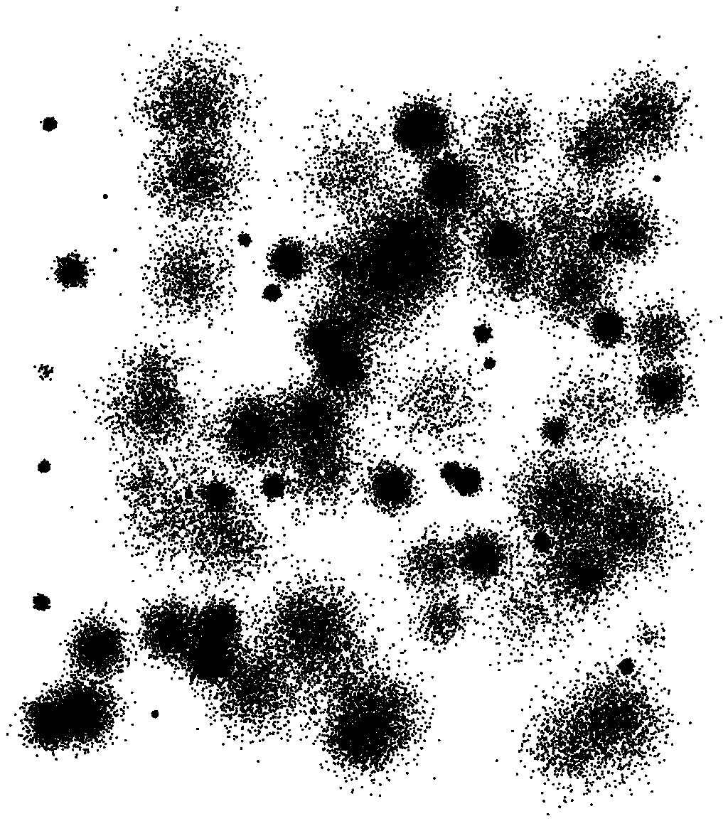
Figure 10: Orig. dataset

Figure 11: Sample 44%

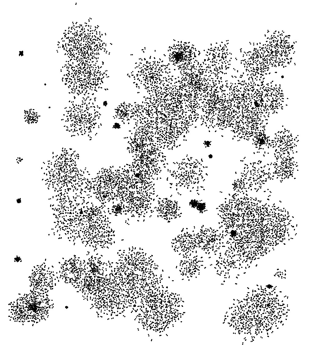
Figure 12: Sample 28%

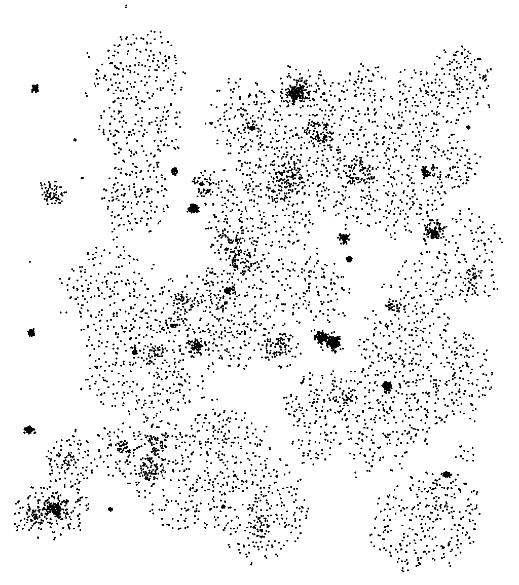
Figure 13: Sample 15%

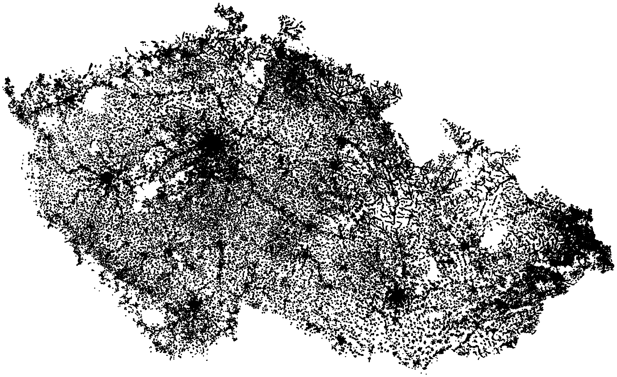
Figure 14: Original dataset

Figure 15: Sample 8%

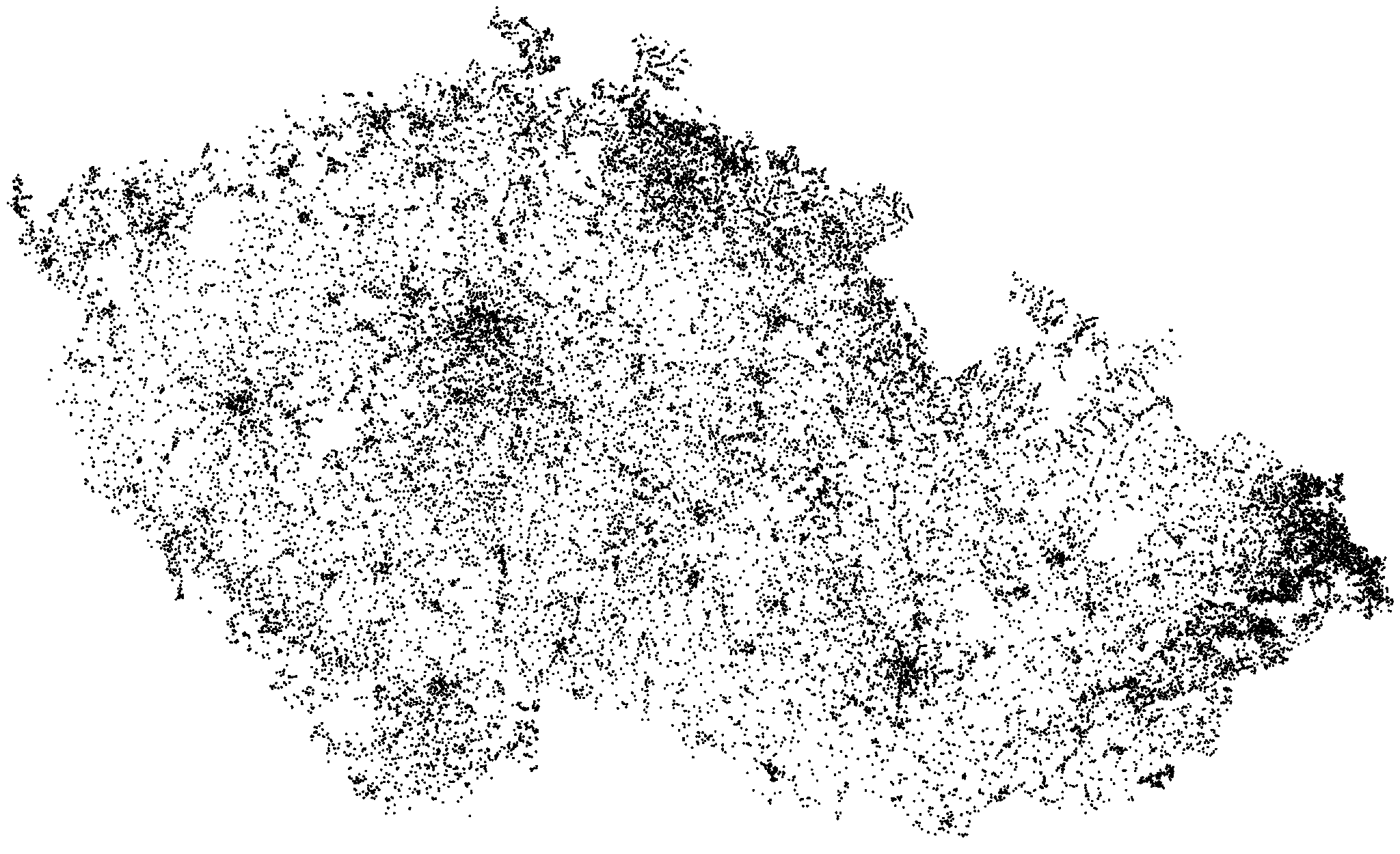
Figure 16: Sample 2%

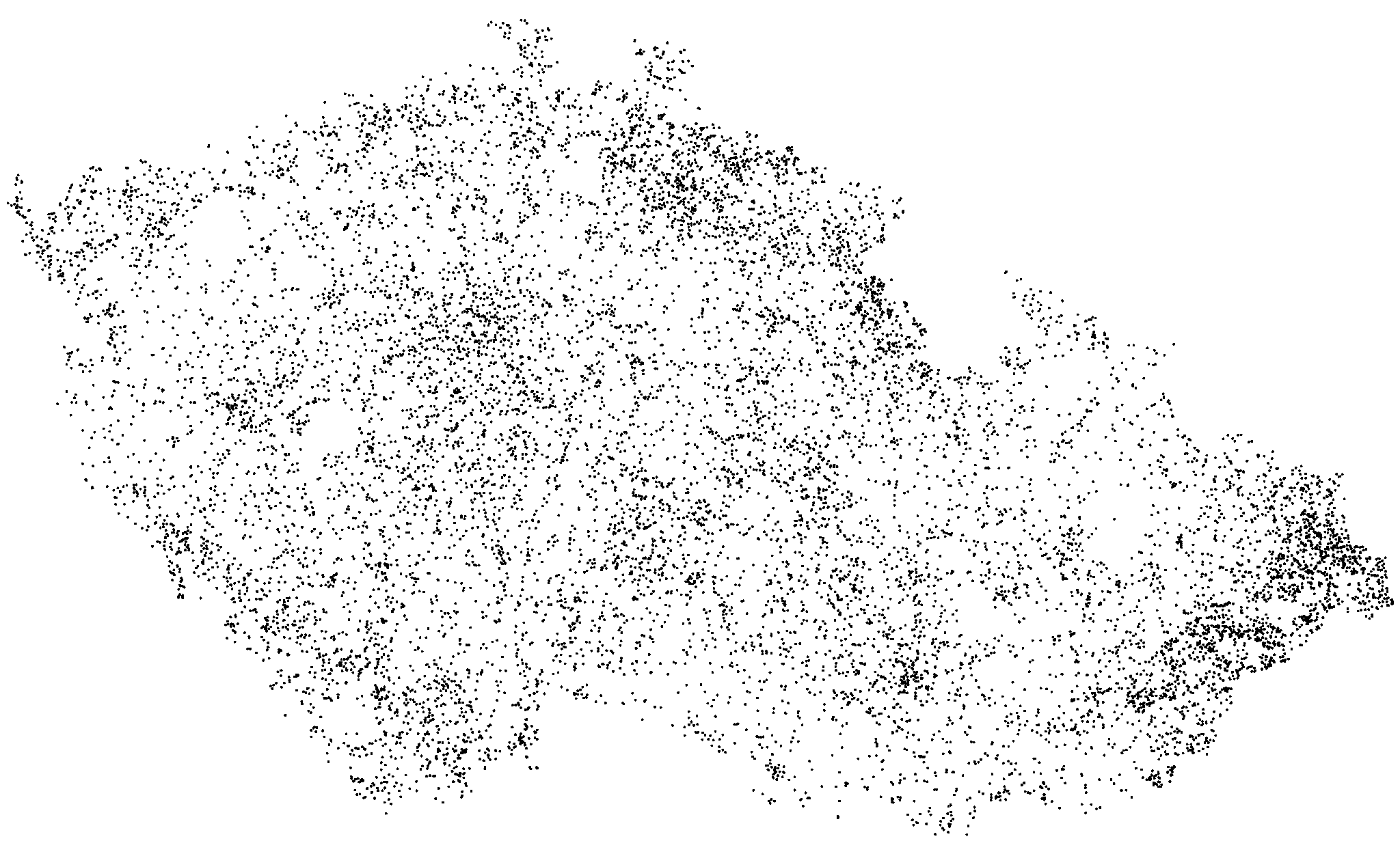
Figure 17: Sample 1%

As may be seen from the figures, the first sample (see Figure 13) preserves the cluster centers precisely. Especially the most dense areas are preserved. The points on the border of clusters and points with higher distance from the cluster centers are removed. The second sample (see Figure 13) with higher radius show a different aspect of the algorithm, because the points were removed mostly from cluster centers while the border points are preserved, but the most dense areas are still preserved. The last sample (see Figure 13) with the highest radius shows that only the most dense cluster centers are still preserved and other clusters are replaced by the points from the whole cluster. Very interesting is that even points which are far from the center of any cluster and might be removed as a noise are preserved if they form a cluster with the neighborhood.

The second experiment uses a real world 2-dimensional dataset which contains all address points in the Czech Republic provided by the government . This data set contains 2,7640,903 address points with coordinates in S-JTSK coordination system (S-JTSK is a coord. system which was used since beginning of the 20th century in Czechoslovakia and the length unit is approximately one meter). The points are distributed more densely in the area of large cities, e.g. the most dense place is in the middle of the image where the capital city Prague is located, but very dense areas are also on the north and south, although the most populated area of the Czech Republic is on the east where Moravian-Silesian region is located. Similarly to the previous experiment we dicretize the distance with step 10. The summary of the data sampling with different radius are depicted in Table 5 and for the visualization see Figures 17-17.

Table 5: Czech Map Dataset Sampling

Log base	Radius	Points	Points %
-	-	2,740,903	100
1.3	50	206,603	8
1.3	100	55,641	2
1.3	200	21,965	1

As may be seen from the figures, visual comparison shows that the most dense parts are still dense and recognizable even when very large reduction is performed. The Figure 17, where only 2% of points is preserved clearly show the largest cities in the Czech Republic and, moreover, shows that the east part of the republic has many densely populated places, and therefore, it is the most dense area preserved.

Remark 2.

We convert the problem of sampling the vector data to the problem of sampling networks as follows; every vector is a node that has an egde to every neighbor (a vector in its neighborhood) and the weight of the edge corresponds to the distance converted to similarity.

4.4 Algorithm complexity

The complexity of the algorithm may be clearly extracted from the pseudo-code. If we suppose that the dataset D contains N objects and the average size of the neighborhood is $M$ then the complexity of the algorithm is $O(NM)$. Usually we may assume that the $M\ll N$ so the complexity is linear. This is done because of the locality of the algorithm. If we think deeper about the algorithm we see that the complexity is highly affected by the complexity of the neighborhood discovery. This is affected by the similarity and proximity functions, but if we suppose that these two functions follow the locality we may divide the problem into two types. First, when we deal with network data, we may suppose that the each node knows its neighbors because we usually have a list of edges for each node. When we deal with vector data the situation is different. In such dataset we know only the information about each vector itself but we have no information about its neighbors. So we must use some data structure which enables fast neighborhood exploration. Many such structures were developed in the past, such as R-Tree and KD-Tree, and their variants or when the data has small dimension we may use Quadrant tree. These structures allow to find neighbors in constant or, in the worst case, logarithmic time so the efficiency of the algorithm is still very good.

5 Conclusions

In this paper we presented our ’work in progress’ in the field of sampling large-scale data. The approach is based on finding the representatives in the input dataset. Measurement of representativeness is done by the analysis of local properties and nearest neighbors. We show in the experiments how we practically apply the method to the weighted networks and vector data. As the key features of the method we consider its applicability for weighted networks, natural scalability and generality.
There are several more tasks to solve in the future work. In particular, carrying out with experiments on large-scale data and comparing with other biased and unbiased methods. Since every dataset requires a different setting it is necessary to make a deeper analysis of the dependencies between parameters of the presented method, processed dataset and expected representative sample. We see the potential especially in the openness of the method to the definitions of similarity, proximity and representativeness. Given that all those functions may be non-symmetric, subject of experiments will also be the directed networks.

6 Acknowledgments

This work was supported by the European Regional Development Fund in the IT4Innovations Centre of Excellence project (CZ.1.05/1.1.00/02.0070), by the Development of human resources in research and development of latest soft computing methods and their application in practice project, reg. no. CZ.1.07/2.3.00/20.0072 funded by Operational Programme Education for Competitiveness, co-financed by ESF and state budget of the Czech Republic, and by SGS, VSB-Technical University of Ostrava, under the grant no. SP2014/110.

References

- [1] N. K. Ahmed, J. Neville, and R. Kompella. Reconsidering the foundations of network sampling. Proc. of WIN, 2010.
- [2] C. Hubler, H.-P. Kriegel, K. Borgwardt, and Z. Ghahramani. Metropolis algorithms for representative subgraph sampling. In Data Mining, 2008. ICDM’08. Eighth IEEE International Conference on, pages 283–292. IEEE, 2008.
- [3] K. Kerdprasop, N. Kerdprasop, and P. Sattayatham. Weighted k-means for density-biased clustering. In Data Warehousing and Knowledge Discovery, pages 488–497. Springer, 2005.
- [4] D. E. Knuth, D. E. Knuth, and D. E. Knuth. The Stanford GraphBase: a platform for combinatorial computing, volume 4. Addison-Wesley Reading, 1993.
- [5] G. Kollios, D. Gunopulos, N. Koudas, and S. Berchtold. Efficient biased sampling for approximate clustering and outlier detection in large data sets. Knowledge and data engineering, ieee transactions on, 15(5):1170–1187, 2003.
- [6] V. Krishnamurthy, M. Faloutsos, M. Chrobak, J.-H. Cui, L. Lao, and A. G. Percus. Sampling large internet topologies for simulation purposes. Computer Networks, 51(15):4284–4302, 2007.
- [7] M. Kudělka, Z. Horák, V. Snášel, P. Krömer, J. Platoš, and A. Abraham. Social and swarm aspects of co-authorship network. Logic Journal of IGPL, 20(3):634–643, 2012.
- [8] J. Leskovec and C. Faloutsos. Sampling from large graphs. In Proceedings of the 12th ACM SIGKDD international conference on Knowledge discovery and data mining, pages 631–636. ACM, 2006.
- [9] A. S. Maiya and T. Y. Berger-Wolf. Sampling community structure. In Proceedings of the 19th international conference on World wide web, pages 701–710. ACM, 2010.
- [10] A. Nanopoulos, Y. Manolopoulos, and Y. Theodoridis. An efficient and effective algorithm for density biased sampling. In Proceedings of the eleventh international conference on Information and knowledge management, pages 398–404. ACM, 2002.
- [11] C. R. Palmer and C. Faloutsos. Density biased sampling: an improved method for data mining and clustering, volume 29. ACM, 2000.
- [12] D. Rafiei. Effectively visualizing large networks through sampling. In Visualization, 2005. VIS 05. IEEE, pages 375–382. IEEE, 2005.
- [13] A. H. Rasti, M. Torkjazi, R. Rejaie, and D. Stutzbach. Evaluating sampling techniques for large dynamic graphs. Univ. Oregon, Tech. Rep. CIS-TR-08, 1, 2008.
- [14] T. Zhang, R. Ramakrishnan, and M. Livny. Birch: A new data clustering algorithm and its applications. Data Mining and Knowledge Discovery, 1(2):141–182, 1997.