Solutions of the Bethe-Salpeter Equation in Minkowski space: a comparative study

Abstract

The Bethe-Salpeter equation for a two-scalar, S-wave bound system, interacting through a massive scalar, is investigated within the ladder approximation. By assuming a Nakanishi integral representation of the Bethe-Salpeter amplitude, one can deduce new integral equations that can be solved and quantitatively studied, overcoming the analytic difficulties of the Minkowski space. Finally, it is shown that the Light-front distributions of the valence state, directly obtained from the Bethe-Salpeter amplitude, open an effective window for studying the two-body dynamics.

1 Introduction

Recently, there has been a renewal of interest in looking for solutions of the Bethe-Salpeter Equation (BSE) in Minkowski space (see, e.g., Refs. [1; 2; 3; 4] and, for earlier studies, see Ref. [5]), since the perspective of establishing a new framework where both bound and scattering states can be investigated in a non perturbative regime is very attractive (let us remind that an integral equation is a non perturbative tool). As is well known, to get solutions in Minkowski space represents a big challenge, since the analytic structure of the relevant quantities, like the irreducible kernel present in BSE and particularly the Bethe-Salpeter amplitude (BSA), has to be explicitly considered. A possible way to overcome such a difficulty is provided by assuming that the BSA have an expression inspired by the perturbation-theory integral representation (PTIR), introduced by N. Nakanishi in the sixties (see Ref.[6] for the textbook presentation of the topic) for describing N-leg transition amplitudes. As emphasized by the name itself of the approach, the Nakanishi integral representation holds in a perturbative regime. For the BSA, one should consider the expression corresponding to the 3-leg transition amplitude. Hence the question if and to what extent actual solutions of the BSE, that have a non perturbative nature, can be expressed through the Nakanishi PTIR.

In the present contribution, we give a brief presentation (see Refs. [3; 4] for details) of the application of the Nakanishi approach for solving the ladder BSE, within a non-explicitly covariant Light-front (LF) framework. The system analyzed is composed by two massive scalars, interacting through a massive scalar, in a bound S-wave state. Let us shortly recall the BS approach (see, e.g., [7] for details).

The 4-point Green’s function (FPGF), $G(x_{1},x_{2};y_{1},y_{2})=<0\,|\,T\{\phi_{1}(x_{1})\phi_{2}(x_{2})\phi_{1}^{+}(y_{1})\phi_{2}^{+}(y_{2})\}\,|\,0>$, fulfills an integral equation: $G=G_{0}~{}+~{}G_{0}~{}{\cal I}~{}G$, where $G_{0}$ is the Green’s function of two free particles and ${\cal I}$ the irreducible kernel, given by the infinite sum of Feynman graphs, that cannot be disconnected after cutting along one line the scalar propagations, but without touching the exchanged-scalar propagations. All the expected contributions can be obtained by iterating the previous integral equation. By inserting a complete Fock basis in the expression of the FPGF and moving to the Fourier space, one can single out the bound state contribution (assuming only one non-degenerate bound state, for the sake of simplicity). Such a contribution to the FPGF appears as a pole, viz.

$$G_{b}(k,q;p_{b})\simeq{i\over(2\pi)^{-4}}~{}\frac{\phi(k;p_{b})~{}\bar{\phi}(k;p_{b})}{2\omega_{b}(p_{0}-\omega_{b}+i\epsilon)}$$ (1)

where $\omega_{b}=\sqrt{M^{2}_{b}+|{\bf p}_{b}|^{2}}$, $p^{2}_{b}=M^{2}_{b}$ and $\phi(k;p_{b})$ is the Fourier transform of the BSA for a bound state, given by $\langle 0|T\{\phi_{1}(x_{1})\phi_{2}(x_{2})\}|p_{b}\,\beta\rangle$. For $p_{0}\to\omega_{b}$ the FPGF is approximated by $G\simeq G_{b}+~{}regular~{}terms$ and one deduces from $G=G_{0}~{}+~{}G_{0}~{}{\cal I}~{}G$ the integral equation determining the BSA for a bound state, viz

$$\phi(k;p_{b},\beta)=G_{0}(k;p_{b},\beta)~{}\int d^{4}q^{\prime}~{}{\cal I}(k,q^{\prime};p_{b})~{}\phi(q^{\prime};p_{b},\beta)$$ (2)

where $G_{0}=i^{2}/\{[(p_{b}/2+k)^{2}-m^{2}+i\epsilon]~{}[(p_{b}/2-k)^{2}-m^{2}+i\epsilon]\}$ with $p_{b}=p_{1}+p_{2}$ and $k=(p_{1}-p_{2})/2$. Notably, the same irreducible kernel, ${\cal I}(k,q^{\prime};p_{b})$, present in the integral equation for the FPGF, is acting.

2 The Nakanishi integral representation of the BS amplitude

The PTIR $N$-leg transition amplitude can be formally written as

$$f_{N}(s)\sum_{\cal G}~{}f_{\cal G}(s)\propto~{}\prod_{h}\int_{0}^{1}dz_{h}\int_{0}^{\infty}d\gamma\frac{\delta(1-\sum_{h}z_{h})~{}\phi_{N}(z,\gamma)}{(\gamma-\sum_{h}z_{h}s_{h})}$$ (3)

where ${\cal G}$ indicates a generic Feynman diagram contributing to the $N$-leg amplitude, and ${\phi}_{N}(z,\gamma)=\sum_{\cal G}\tilde{\phi}_{\cal G}(z,\gamma)$. For the $3$-leg case, the so-called vertex function, one has

$$f_{3}(s)=\int_{-1}^{1}dz\int_{-\infty}^{\infty}d\gamma\frac{\phi_{3}(z,\gamma)}{\gamma-{p^{2}\over 4}-k^{2}-zk\cdot p-i\epsilon}$$ (4)

Within the BS framework, can such an elegant expression be exploited for modeling the BSA (see, e.g.,[5; 1; 2; 3; 4])? In particular, if the BSA for both bound and scattering states [3] has actually such a form, then one can determine the Nakanishi weight function, $\phi_{3}$, through an integral equation (indeed one can construct two integral equations as explained in what follows), that can be directly deduced from the BSE. This achievement allows one to answer the question: can the Nakanishi representation of the vertex function, elaborated in perturbation theory, be used in a non perturbative realm, as the BS framework does (recall that BSE is an integral equation)?

A suitable integral equation for the relevant Nakanishi weight function can be obtained by applying the so-called LF projection method (see, e.g., [3; 8] and references quoted there in). This amounts to integrate the BSE on the LF variable $k^{-}=k^{0}+k_{z}$, but in order to perform the needed integration one has to know the analytic structure of the unknown BSA. Let us take the Nakanishi vertex function as an Ansatz for the BS amplitude, $\Phi_{b}(k,p)$ and then integrate it on the $k^{-}$. As a result, then one gets the valence component of the state of the interacting system (after expanding it onto the Fock basis) [1; 3]

$$\psi_{n=2}(\xi,k_{\perp})={p^{+}\over\sqrt{2}}~{}\xi(1-\xi)\int{dk^{-}\over 2\pi}\Phi_{b}(k,p)={\xi(1-\xi)\over\sqrt{2}}\int_{0}^{\infty}d\gamma^{\prime}~{}\frac{g_{b}(\gamma^{\prime},1-2\xi;\kappa^{2})}{[\gamma^{\prime}+k_{\perp}^{2}+\kappa^{2}+\left(2\xi-1\right)^{2}{M^{2}_{b}\over 4}-i\epsilon]^{2}}$$ (5)

where $g_{b}$ is the Nakanishi weight function (adopting the standard notation of Refs. [3; 4], see also [1; 2] for the explicitly covariant LF approach). Applying the LF projection to both sides of the BSE, one obtains

$$\int_{0}^{\infty}d\gamma^{\prime}\frac{g_{b}(\gamma^{\prime},z;\kappa^{2})}{[\gamma^{\prime}+\gamma+z^{2}m^{2}+(1-z^{2})\kappa^{2}-i\epsilon]^{2}}=\int_{0}^{\infty}d\gamma^{\prime}\int_{-1}^{1}dz^{\prime}~{}V^{LF}_{b}(\gamma,z;\gamma^{\prime},z^{\prime})g_{b}(\gamma^{\prime},z^{\prime};\kappa^{2}).$$ (6)

where $\kappa^{2}=m^{2}-M^{2}_{b}/4$, and $V^{LF}_{b}(\gamma,z;\gamma^{\prime},z^{\prime})$ is determined by the irreducible kernel ${\cal I}(k,k^{\prime},p)$. Moreover, if one assumes that the uniqueness theorem of the Nakanishi weight function (see Ref. [6] for the demonstration within the PTIR framework) holds also in the non perturbative regime, one can deduce from Eq. (6) a simpler integral equation for the weight function, viz

$$g_{b}(\gamma,z;\kappa^{2})=~{}\int_{0}^{\infty}d\gamma^{\prime}\int_{-1}^{1}dz^{\prime}\;{\cal V}_{b}(\gamma,z;\gamma^{\prime},z^{\prime};\kappa^{2})g_{b}(\gamma^{\prime},z^{\prime};\kappa^{2})$$ (7)

where ${\cal V}_{b}(\gamma,z;\gamma^{\prime},z^{\prime};\kappa^{2})$ is a new kernel, properly related to $V^{LF}_{b}(\gamma,z;\gamma^{\prime},z^{\prime})$ (see [3; 4]) .

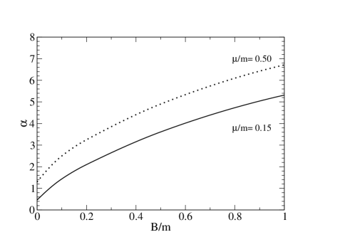
Figure 1: Left panel: Values of the coupling constant $\alpha=g^{2}/(m^{2}16\pi)$ vs the binding energy $B/m$ for two values of the exchanged scalar mass $\mu/m=0.15,~{}0.50$. Right panel: $\Delta g(\gamma,z;\kappa^{2})=~{}\left|g_{U}(\gamma,z;\kappa^{2})-g_{V}(\gamma,z;\kappa^{2})\right|$ for$B/m=1.0$ and $\mu/m=0.5$.

3 Results and conclusions

The two integral equations, (6) and (7), have been carefully investigated, in ladder approximation, in Ref. [4], and the numerical results have been compared to the ones in Ref. [5] (where the uniqueness theorem was exploited, but with standard variables in Minkowski space) and in Ref. [1]. The quantitative studies proceed by assigning a value to the binding energy of the system, $B/m=2-M_{b}/m$, and then determining i) the coupling constant $\alpha=g^{2}/(m^{2}16\pi)$ (recall that the interacting Lagrangian is ${\cal L}=g\phi^{2}\chi$) and the corresponding Nakanishi weight function. The values of $\alpha$, for different values of the exchanged scalar mass $\mu/m$, agree very accurately with the ones in Refs [5; 1], and they are illustrated in Fig. 1, left panel (for a detailed analysis see Ref. [4]). In the right panel of Fig. 1, it is presented for $B/m=1.0$ and $\mu/m=0.5$ the difference between the Nakanishi weight function obtained from Eq. (6), shortly indicated by $g_{V}$, and the one obtained from Eq. (7), $g_{U}$. In general, the differences are quite small (for more comparisons see Ref. [4]), and it should be reminded that $g_{b}(\gamma,z;\kappa^{2})$ must vanish at the end-points $z=\pm 1$ and quickly fall off for increasing $\gamma/m$. From the valence wave function, Eq. (5), one can calculate [4] i) the probability of the valence component, $P_{val}$, ii) the LF distribution of the longitudinal-momentum fraction, $\phi(\xi)$, and iii) LF distribution of the transverse momentum, ${\cal P}(\gamma)$, given by

$$\phi(\xi)={1\over(2\pi)^{3}}{1\over 2~{}\xi(1-\xi)}~{}\int d{\bf k}_{\perp}~{}\psi^{2}_{n=2/p}(\xi,k_{\perp})~{},~{}{\cal P}(\gamma)={1\over 2(2\pi)^{3}}\int_{0}^{1}{d\xi\over 2~{}\xi(1-\xi)}~{}\int_{0}^{2\pi}d\phi\psi^{2}_{n=2/p}(\xi,k_{\perp})$$ (8)

Those distributions, shown in Fig. 2 for some values of $B/m$ and $\mu/m=0.5$, open an interesting window on the internal dynamics of the system. In particular, from the present, preliminary analysis, the $\gamma/m$ tail of the transverse-momentum distribution is governed by the ladder kernel, providing a power-like behavior. This will be thoroughly investigated elsewhere [9].

In conclusion, combining the Nakanishi integral representation of the BS amplitude and the LF projection one can afford the investigation of the BSE in Minkowski space. In perspective, this can allow to develop applications in different areas, from solid state physics to hadronic physics. Calculations are in progress for i) the scattering length and ii) the cross-box contribution with the uniqueness theorem.

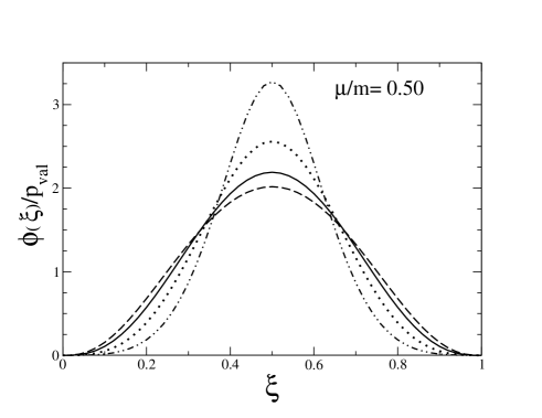
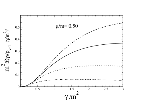
Figure 2: Left panel: the LF longitudinal-momentum fraction distribution, $\phi(\xi)$, vs the longitudinal-momentum fraction $\xi=k^{+}/M$. Dash-double-dotted line: $B/m=0.20$. Dotted line: $B/m=0.50$. Solid line: $B/m=1.0$. Dashed line: $B/m=2.0$. (N.B. $\int^{1}_{0}d\xi~{}\phi(\xi)=P_{val}$).(After from Ref.[4]) Right panel: the same of the left panel but for the LF transverse-momentum distribution, ${\cal P}(\gamma)~{}(\gamma/m^{2})^{3}$ vs $\gamma/m^{2}$ (recall that $\gamma=k_{\perp}^{2}$). (Adapted from Ref.[4]).

T.F acknowledges the partial financial support from the Conselho Nacional de Desenvolvimento Científico e Tecnológico (CNPq), the Fundação de Amparo à Pesquisa do Estado de São Paulo (FAPESP)

References

- [1] J. Carbonell and V. Karmanov: Solving Bethe-Salpeter equation in Minkowski space. Eur. Phys. Jou. A A 27, 1 (2006).
- [2] J. Carbonell and V. Karmanov: Cross-ladder effects in Bethe-Salpeter and light-front equations. Eur. Phys. Jou. A A 27, 11 (2006).
- [3] T. Frederico, G. Salmè and M. Viviani: Two-body scattering states in Minkowski space and the Nakanishi integral representation onto the null plane. Phys. Rev. D 85, 036009 (2012).
- [4] T. Frederico, G. Salmè and M. Viviani: Quantitative studies of the homogeneous Bethe-Salpeter Equation. in Minkowski space. Phys. Rev. D 89, 016010 (2014) and arXiv 1312.0521.
- [5] K. Kusaka, K. Simpson, A.G. Williams: Solving the Bethe-Salpeter equation for bound states of scalar theories in Minkowski space. Phys. Rev. D 56, 5071 (1997).
- [6] N. Nakanishi; Graph Theory and Feynman Integrals. Gordon and Breach, New York, 1971.
- [7] C. Itzykson, J.B. Zuber. Quantum Field Theory. Dover Publications (2006).
- [8] T. Frederico and G. Salmè. Projecting the Bethe-Salpeter Equation onto the Light-Front and Back: A Short Review. Few-Body Syst. 49, 163 (2011).
- [9] T. Frederico, G. Salmè and M. Viviani. To be published.