A route to thermalization in the $\alpha$-Fermi-Pasta-Ulam system

Abstract

We study the original $\alpha$-Fermi-Pasta-Ulam (FPU) system with $N=16,32$ and $64$ masses connected by a nonlinear quadratic spring. Our approach is based on resonant wave-wave interaction theory, i.e. we assume that, in the weakly nonlinear regime (the one in which Fermi was originally interested), the large time dynamics is ruled by exact resonances. After a detailed analysis of the $\alpha$-FPU equation of motion, we find that the first non trivial resonances correspond to six-wave interactions. Those are precisely the interactions responsible for the thermalization of the energy in the spectrum. We predict that for small amplitude random waves the time scale of such interactions is extremely large and it is of the order of $1/\epsilon^{8}$, where $\epsilon$ is the small parameter in the system. The wave-wave interaction theory is not based on any threshold: equipartition is predicted for arbitrary small nonlinearity. Our results are supported by extensive numerical simulations. A key role in our finding is played by the Umklapp (flip over) resonant interactions, typical of discrete systems. The thermodynamic limit is also briefly discussed.

Nonlinear waves — FPU recurrence — resonant interactions

1 Introduction

The Fermi-Pasta-Ulam (FPU) chains is a simple mathematical model introduced in the fifties to study the thermal equipartition in crystals [1]. The model consists of $N$ identical masses each one connected by a nonlinear spring; the elastic force can be expressed as a power series in the spring deformation $\Delta x$:

$$F=-\gamma\Delta x+\alpha\Delta x^{2}+\beta\Delta x^{3}+...,$$ (1)

where $\gamma,\alpha$ and $\beta$ are elastic, spring dependent, constants. The $\alpha$-FPU chain, the system studied herein, corresponds to the case of $\alpha\neq 0$ and $\beta=0$. Fermi, Pasta and Ulam integrated numerically the equation of motion and conjectured that, after many iterations, the system would exhibit a thermalization, i.e.​ a state in which the influence of the initial modes disappears and the system becomes random, with all modes excited equally (equipartition of energy) on average. Contrary to their expectations, the system exhibited a very complicated quasi-periodic behavior. This phenomenon has been named “FPU recurrence” and this finding has spurred many great mathematical and physical discoveries such as integrability [2] and soliton physics [3].

More recently, very long numerical simulations have shown a clear evidence of the phenomenon of equipartition, see for instance [4] and references therein. Yet, despite substantial progresses on the subject  [5, 6, 7, 8, 9, 10], up to our knowledge no complete understanding of the original problem has been achieved so far and the numerical results of the original $\alpha$-FPU system remain largely unexplained from a theoretical point of view. More precisely, the physical mechanism responsible for a first metastable state [4] and the observation of equipartition for very large times have not been understood.

In this manuscript, we study the FPU problem using an approach based on the nonlinear interaction of weakly nonlinear dispersive waves. Our main assumption is that the irreversible transfer of energy in the spectrum in a weakly nonlinear system is achieved by exact resonant wave-wave interactions. Such resonant interactions are the base for the so called wave turbulence theory  [11, 12] and are responsible for the phenomenon of thermalization. Specifically, we will show that in the $\alpha$-FPU system six-wave resonant interactions are responsible for an effective irreversible transfer of energy in the spectrum.

2 The Model

The equation of motion for a chain of $N$ identical particles of mass $m$, subject to a force of the type in (1) with $\alpha\neq 0$ and $\beta=0$, has the following form:

$$m\ddot{q}_{j}=\left(q_{j+1}+q_{j-1}-2q_{j}\right)\left(\gamma+\alpha(q_{j+1}-q_{j-1})\right),$$ (2)

with $j=0,1,..,N-1$. Here $q_{j}(t)$ is the displacement of the particle $j$ from the equilibrium position. We consider periodic boundary conditions, i.e. $q_{N}=q_{0}$. Our approach is developed in Fourier space and the following definitions of the direct and inverse Discrete Fourier Transform are adopted:

$$Q_{k}=\frac{1}{N}\sum_{j=0}^{N-1}q_{j}e^{-i2\pi kj/N},\;q_{j}=\sum_{k=-N/2+1}^{N/2}Q_{k}e^{i2\pi jk/N},$$ (3)

where $k$ are discrete wavenumbers and $Q_{k}$ are the Fourier amplitudes.

2.1 Normal modes

We then introduce the complex amplitude of a normal mode $a_{k}=a(k,t)$ as:

$$a_{k}=\frac{1}{\sqrt{2\omega_{k}}}(P_{k}-i\omega_{k}Q_{k}),$$ (4)

where $\omega_{k}=\omega(k)$ is the angular frequency related to wave-numbers as follows:

$$\omega_{k}=2\sqrt{\frac{\gamma}{m}}|\sin(\pi k/N)|,$$ (5)

and $P_{k}$ is the momentum, $P_{k}=\dot{Q}_{k}$. Substituting the above definitions into the equation of motion (2) and introducing the nondimensional variables

$$\begin{split}a^{\prime}_{k}=\frac{(\gamma/m)^{1/4}}{\sqrt{\sum_{k}\omega_{k}|a_{k}(t=0)|^{2}}}a_{k},\;\;\;t^{\prime}=\sqrt{\frac{\gamma}{m}}t,\;\;\ \omega_{k}^{\prime}=\sqrt{\frac{m}{\gamma}}\omega_{k},\end{split}$$ (6)

we get the following evolution equation:

$$\begin{split}&i\frac{\partial a_{1}}{\partial t}=\omega_{1}a_{1}+\epsilon\sum\limits_{k_{2},k_{3}}V_{1,2,3}\bigg{(}a_{2}a_{3}\delta_{1,2+3}+2a_{2}^{*}a_{3}\delta_{1,3-2}+\\ &+a_{2}^{*}a_{3}^{*}\delta_{1,-2-3}\bigg{)},\end{split}$$ (7)

where primes have been omitted for brevity and the summation on $k_{2}$ and $k_{3}$ is intended from $-N/2+1$ to $N/2$; $a_{i}=a(k_{i},t)$, $\delta_{i,j}=\delta_{k_{i},k_{j}}$ is the Kronecker delta that should be understood with “modulus $N$”, i.e. it is also equal to one if the argument differs by $N$. The dispersion relation becomes now $\omega_{k}=2|\sin(\pi k/N)|$. The matrix $V_{1,2,3}$ weights the transfer of energy between wave numbers $k_{1}$, $k_{2}$ and $k_{3}$ and is given by:

$$V_{1,2,3}=-\frac{1}{2\sqrt{2}}\frac{\sqrt{\omega_{1}\omega_{2}\omega_{3}}}{\mbox{sign}[\sin(\pi k_{1}/N)\sin(\pi k_{2}/N)\sin(\pi k_{3}/N)]}.$$ (8)

The parameter $\epsilon$, given by

$$\epsilon=\frac{\alpha}{m}\left(\frac{\gamma}{m}\right)^{1/4}{\sqrt{\sum_{k}\omega_{k}|a_{k}(t=0)|^{2}}},$$ (9)

is the only free parameter of the model. If $\epsilon=0$ the system is linear; in the present manuscript we are interested in the weakly nonlinear regime, i.e. $\epsilon\ll 1$.

2.2 Absence of three wave resonant interactions and the role of the canonical transformation

Equation (7), which has a Hamiltonian structure with canonical variables $\{ia_{k},a_{k}^{*}\}$, describes the time evolution of the amplitudes of the normal modes of the $\alpha$-FPU system. It is characterized by a quadratic nonlinearity, i.e. a three-wave interaction system. Wave numbers $k_{1}$, $k_{2}$ and $k_{3}$ are called resonant if they satisfy the following equations:

$$k_{1}\pm k_{2}\pm k_{3}{\overset{N}{=}}0,\;\;\;\omega_{1}\pm\omega_{2}\pm\omega_{3}=0,$$ (10)

where the ${\overset{N}{=}}$ sign means “equal modulus $N$”, i.e. wave numbers may scatter over the edge of the Brillouin zone because of the Umklapp (flip over) scattering [13]. Using Prosthaphaeresis formulas one can show that it is impossible to find non zero $k_{1}$, $k_{2}$ and $k_{3}$ satisfying (10) with $\omega(k)$ given in (5). This observation leads to a first important consideration: the Fourier modes $a_{k}$ in the $\alpha$-FPU system can be divided into free and bound modes. To illustrate the concept of the bound modes, we refer to the classical hydrodynamic example of the Stokes wave in surface gravity waves, see e.g. [14]. The Stokes wave is a solution of the Euler equations and is characterized by a primary sinusoidal wave plus higher harmonics whose amplitudes depend on the primary wave. Those higher harmonics are bound to the primary free sinusoidal mode and they do not obey to the linear dispersion relation. Cnoidal waves and solitons are similar objects: they are characterized by a large number of harmonics that are not free to interact with each other. In the light of the above comments, we then make the following statement: the equipartition phenomenon is not to be expected for the Fourier modes of the original variables $a(k,t)$ or $Q(k,t)$, but only for those that are free to interact. The rest of the modes in the spectrum do not have an independent dynamics and are phase-locked to the free ones. The question is then how to build a spectrum characterized only by free modes. From a theoretical point of view, the problem can be attacked by removing via an ad hoc canonical transformation all interactions that are not resonant. The transformation inevitably generates higher order interactions which may or may not be resonant. If those are not resonant, then a new transformation can be applied to remove them; in principle, such operation can be iterated up to an infinite order in nonlinearity, as long as no resonant interactions are encountered. In the presence of resonant interactions, the transformation diverges because of the classical small divisor problem [15].

For the case of $\alpha$-FPU, the following transformation from canonical variables $\{ia_{k},a_{k}^{*}\}$ to $\{ib_{k},b_{k}^{*}\}$

$$\begin{split}&a_{1}=b_{1}+\epsilon\sum\limits_{k_{2},k_{3}}(A_{1,2,3}^{(1)}b_{2}b_{3}\delta_{1,2+3}+A_{1,2,3}^{(2)}b_{2}^{*}b_{3}\delta_{1,3-2}+\\ &+A_{1,2,3}^{(3)}b_{2}^{*}b_{3}^{*}\delta_{1,-2-3})+O(\epsilon^{2})\end{split}$$ (11)

removes the triad interactions in (7) and introduces higher order nonlinearity. Here

$$A_{1,2,3}^{(1)} = V_{1,2,3}/(\omega_{3}+\omega_{2}-\omega_{1}),$$

$$A_{1,2,3}^{(2)} = 2V_{1,2,3}/(\omega_{3}-\omega_{2}-\omega_{1}),\$$

$$A_{1,2,3}^{(3)} = V_{1,2,3}/(-\omega_{3}-\omega_{2}-\omega_{1}).$$

Note that the denominators are never zero because of the non existence of triad resonant interactions. Higher order terms in (11) will be considered latter on and will involve four, five and six wave interactions. These higher order terms will play a crucial role in the foregoing analyses. The procedure for calculations of such canonical transformations is well established [16] and may be implemented, for example, by usage of diagrammatic technique, as was done in [17].

In order to present a physical interpretation of the canonical transformation, we can write it in terms of the original variable $q_{j}(t)$. Using (3) and (4), the displacement of the masses can be written in the following form:

$$q_{j}(t)=i\sum_{k}\left[\frac{a_{k}}{\sqrt{2\omega_{k}}}e^{i2\pi jk/N}-c.c.\right],$$ (12)

where $c.c.$ stands for complex conjugate. We now plug (11) in (12) and for simplicity we assume that the free modes are characterized by a monochromatic wave centered in $k_{0}$ of the form $b(k,t)=|\bar{b}|\delta_{k,k_{0}}e^{-i(\omega_{k_{0}}t-\phi_{k_{0}})}$, with $\omega_{k_{0}}=2|\sin(\pi k_{0}/N)|$, $|\bar{b}|$ a constant and $\phi_{k_{0}}$ an arbitrary phase; after some algebra, the following result is obtained for the displacement (see also [19]):

$$q_{j}(t)=A\sin(\theta)+\epsilon B\sin(2\theta)+O(\epsilon^{2}),$$ (13)

with $\theta=2\pi k_{0}j/N-\omega_{0}t+\phi_{k_{0}}$, $A=-2|\bar{b}|/\sqrt{2\omega_{k_{0}}}$, $B=2V_{2k_{0},k_{0},k_{0}}\sqrt{2\omega_{k_{0}}}|\bar{b}|^{2}/(-4\omega_{k_{0}}^{2}+\omega^{2}_{2k_{0}})$. Note that $B$ is proportional to $A^{2}$ and the second harmonic $2k_{0}$ does not oscillate with frequency $\omega(2k_{0})$ but with $2\omega(k_{0})$, i.e. it does not obey to the linear dispersion relation. Higher order terms in the canonical transformation would bring higher harmonics. It is clear that the spectrum associated to the variable $b_{k}$ (in the present case, a single mode) is different from the one associated to the variable $a_{k}$ or $Q_{k}$ (where multiple bound harmonics appear). Equation (13) is nothing but the second order Stokes series solution of the the $\alpha$-FPU system. The initial stage of the $\alpha$-FPU system initialized by a single mode $k_{0}$ would then be characterized by the generation of the harmonics of the type in equation (13).

3 The reduced dynamical equation and exact resonances

We now turn our attention to the dynamical equation that results after the canonical transformation has been performed; the equation reads:

$$\begin{split}&i\frac{\partial b_{1}}{\partial t}=\omega_{1}b_{1}+\epsilon^{2}\sum\limits_{k_{2},k_{3},k_{4}}T_{1,2,3,4}b_{2}^{*}b_{3}b_{4}\delta_{1+2,3+4}+O(\epsilon^{3}).\end{split}$$ (14)

Note that similar terms including the Kroneker deltas $\delta_{1,3+4+2},\delta_{1,-3-4-2},\delta_{1,4-3-2}$ should also appear in equation (14) as a result of the transformation (11); however, those terms are not resonant and can be removed by higher order terms in the transformation. The matrix $T_{1,2,3,4}$ has an articulated analytical form which depends on $V_{1,2,3}$ and is given for example in [17] or [18]. Due to the Hamiltonian structure of the original system, $T_{1,2,3,4}$ has the following symmetries $T_{1,2,3,4}=T_{2,1,3,4}=T_{3,4,1,2}$. We underline that the same equation but with a different matrix $T_{1,2,3,4}$ can be obtained directly for the so called $\beta$-FPU or for the $\alpha+\beta$ -FPU chains. If higher order terms are neglected, the equation admits a Birkhoff normal form [21] (see also [22]). Equation (14), with different linear dispersion relation, different matrix $T_{1,2,3,4}$ and with integrals instead of sums, is the equivalent of the Zakharov equation for one directional water waves [20].

Equation (14) describes the reduced $\alpha$-FPU model where three-wave interactions have been removed by the canonical transformation (11). The resonant interactions associated with equation (14) are described by the following 4-wave resonant conditions:

$$k_{1}+k_{2}-k_{3}-k_{4}{\overset{N}{=}}0,\;\;\;\omega_{1}+\omega_{2}-\omega_{3}-\omega_{4}=0.$$ (15)

Solutions for $k_{i}\in\mathbb{Z}$ and $N=16$ or $32$ or $64$ particles, like in the original FPU problem, are reported below.
Trivial solutions. Trivial resonances are obtained when all wave numbers are the same or when:

$$\begin{split}k_{1}=k_{3},\;k_{2}=k_{4},\end{split}$$ (16)

with permutations of 3 and 4. These trivial solutions are responsible for a nonlinear frequency shift and do not contribute to the energy transfer between modes, as discussed for example in [12].
Nontrivial solutions. Nontrivial resonances exist and are the result of the following scattering process: when three waves interact to generate a fourth one, it can happen that the latter is characterized by a $k\not\in[-N/2+1,...,N/2]$, i.e. outside the Brillouin zone. The system flips back this energy into a mode contained in the domain; as mentioned, this is known as Umklapp scattering process [13, 23]. These resonant modes have the following structure:

$$(k_{1},k_{2},-k_{1},-k_{2}),$$ (17)

with $k_{1}+k_{2}=mN/2$ and $m=0,\pm 1,\pm 2.$ It is instructive to give an example: let us consider a chain of $N$=32 masses; the maximum wave-number accessible is then $k_{max}=16$. One of the quadruplets satisfying the resonant condition (15) is $k_{1}=2$, $k_{2}=14$, $k_{3}=-14$, $k_{4}=30$. The first three wave-numbers are contained in the domain, while $k_{4}$ is outside. The system will interpret $k_{4}=30$ as $k_{4}\rightarrow k_{4}-N=-2$.

In order to account for an effective energy mixing, the quadruplets (four modes satisfying the resonant conditions) should be interconnected, i.e. single wave numbers should belong to different quartets. However, a careful and straightforward analysis of equation (17) reveals that resonant quartets are not interconnected, that is, all of the quartets are isolated: if one puts energy into one of the quartets, and only weakly nonlinear resonant interactions are allowed, the energy will remain in the quartet. The above results has the important consequence that the four-wave interactions in the $\alpha$-FPU model cannot possibly lead to equipartition of energy.

An efficient mixing mechanism should be searched by extending to higher order the canonical transformation. Five-wave interactions are non resonant and can be removed by an appropriate choice of the higher order terms in (11). The resulting evolution equation for $b_{1}$ is a refinement of equation (14) and it has the form:

$$\begin{split}&i\frac{\partial b_{1}}{\partial t}=\omega_{1}b_{1}+\epsilon^{2}\sum T_{1,2,3,4}b_{2}^{*}b_{3}b_{4}+\\ &+\epsilon^{4}\sum\limits W_{1,2,3}^{4,5,6}b_{2}^{*}b_{3}^{*}b_{4}b_{5}b_{6}\delta_{1+2+3,4+5+6}+O(\epsilon^{5}).\end{split}$$ (18)

The explicit form of the matrix $W_{1,2,3}^{4,5,6}$, see for details [12, 24], is not necessary for the discussion of our results. Note that the four-wave interactions cannot be removed because, even though they do not contribute to the spreading of energy in the spectrum, they are resonant and a canonical transformation suitable for removing those modes would diverge.

For $N=16$ or $32$ or $64$ we have found that solutions of the following six-wave resonant conditions

$$\begin{split}k_{1}+k_{2}+k_{3}-k_{4}-k_{5}-k_{6}&{\overset{N}{=}}0,\\ \omega_{1}+\omega_{2}+\omega_{3}-\omega_{4}-\omega_{5}-\omega_{6}&=0,\end{split}$$ (19)

exist for $k_{i}\in\mathbb{Z}$ and we report them below.

Trivial resonances. Trivial resonances are obtained when all six wave numbers are the same or when

$$k_{1}=k_{4},\;k_{2}=k_{5},\;k_{3}=k_{6},$$ (20)

with all permutations of indices 4,5,6. These trivial solutions are responsible only for a nonlinear frequency shift.
Nontrivial symmetric resonances. These resonances are over the edge of the Brillouin zone and are given by:

$$(k_{1},k_{2},k_{3},-k_{1},-k_{2},-k_{3}),$$ (21)

with $k_{1}+k_{2}+k_{3}=mN/2$ and $m=0,\pm 1,\pm 2,...$   .
Nontrivial quasi-symmetric resonances. These resonances over the edge of the Brillouin zone are characterized by one repeated wave number:

$$(k_{1},k_{2},k_{3},-k_{1},-k_{2},k_{3}),$$ (22)

with $k_{1}+k_{2}=mN/2$, $m=0,\pm 1,\pm 2,...$ and all permutations of the indices. We have not found any other integer solutions to the resonant condition (19) for $N=16,32,64$, other than those in (20), (21) and (22).

Those resonant sextuplets are interconnected, therefore they represent an efficient mechanism of spreading energy in the spectrum. Because of the existence of these exact resonant process, we expect the equipartition to take place.

4 Estimation of the equipartition time scale

Thermal equilibrium is a statistical concept; therefore, an equation for the time evolution of the average spectral energy density is required. Within the wave turbulence theory, such equation is called kinetic equation. There are many techniques for deriving it that are object of intensive studies. We are mainly interested in the estimation of the time scale of equipartition; therefore, only the key steps are here considered (details can be found in [11]). We introduce the wave action, $n_{k}=n(k,t)$, defined as $\langle b_{1}b_{2}^{*}\rangle=n_{1}\delta_{1,2}$, where the brackets indicate ensemble averages and the $\delta_{1,2}$ is the Kronecker delta, the latter arising from the assumption of homogeneity of the wave field. In order to derive the evolution equation for $n_{1}$, equation (18) is multiplied by $b_{1}^{*}$ and the ensemble averages are taken. The time evolution of the $n_{1}$ depends on the six-order correlator $\langle b_{1}^{*}b_{2}^{*}b_{3}^{*}b_{4}b_{5}b_{6}\rangle$ whose time evolution will be a function of higher order correlators; this is the classical BBGKY hierarchy problem. The time evolution of the six-order correlator turns out to be proportional to $\epsilon^{4}W_{1,2,3}^{4,5,6}$. Indeed, assuming that the waves obey Gaussian statistics, we decompose the higher order correlators into products of second order correlators and, after taking the large time limit, the six order correlator may be obtained explicitly. The result is then plug into the equation for the time evolution of $n_{k}$, resulting in a collision integral proportional to $(\epsilon^{4}W_{1,2,3}^{4,5,6})^{2}$ (see for example equation (6.89) in [12]). Consequently, the time evolution of the spectral energy density in the $\alpha$-FPU problem is proportional to $1/\epsilon^{8}$. This is the main theoretical result of our work which, as it will be shown, is supported by numerical simulations.

5 Relation to the Toda Lattice

Before showing our numerical simulation results, it is instructive to make a connection between the $\alpha$-FPU and the integrable Toda system [25] (see also [26] for a normal mode approach to the problem). In [4] it has been shown that the $\alpha$-FPU can be seen as a perturbation of the integrable Toda lattice, see also [27]. For the sake of clarity, we report this argument. We consider the general Hamiltonian for a discrete lattice

$$H(p,q)=\frac{1}{2}\sum_{j=1}^{N}p_{j}^{2}+\sum_{i=1}^{N}V(q_{j+1}-q_{j});$$ (23)

the potential $V$ for the $\alpha$-FPU case is given by

$$V(r)=\frac{r^{2}}{2}+\varepsilon\frac{r^{3}}{3}\,.$$ (24)

For the Toda lattice instead $V$ results in

$$V(r)=V_{0}(e^{\lambda r}-1-\lambda r),$$ (25)

with $V_{0}$ and $\lambda$ free parameters. For the particular choice of $V_{0}=1/(4\varepsilon^{2})$ and $\lambda=2\varepsilon$, upon Taylor expanding the exponential in the Toda lattice for small $\varepsilon$, we obtain:

$$V(r)=\frac{r^{2}}{2}+\varepsilon\frac{r^{3}}{3}+\varepsilon^{2}\frac{r^{4}}{6}+\dots\ ,$$ (26)

that shows the $\alpha$-FPU coincides with the Toda Lattice up to the order of $\epsilon$, see eqs. (24) and (26).

Having made this introduction, using our approach based on resonant interactions and, following the fundamental work by Zakharov and Shulmann [28], we are able to discern between integrable and nonintegrable dynamics. We underline that the Toda lattice has the same linear dispersion relation as the $\alpha$-FPU and, therefore, the possible resonant manifolds, being based on linear frequencies, are exactly the same. How then is it possible to explain that the Toda lattice never thermalizes while the FPU does? For the Toda lattice, the same canonical transformation as in (11) can be performed and the three wave interactions be removed (those correspond to the term proportional to $\epsilon$ in the potential in equation (26)). The equation of motion in Fourier space, neglecting higher order terms, becomes the same as the one in equation (14), with the only difference that the matrix $T_{1,2,3,4}$ is now modified due to the existence of the term proportional to $\varepsilon^{2}$ in the potential (26); such term is absent in the potential of the $\alpha$-FPU. A straightforward but lengthy calculation shows that the matrix $T_{1,2,3,4}$ for the Toda lattice is identically zero, once calculated on the resonant manifold. Indeed, this result has very profound origins and is based on the fundamental work by Zakharov and Shulmann [28], where it is shown that for an integrable system, either there are no resonances or all the scattering matrices are zero at all orders on the resonant manifold. In principle an infinite order canonical transformation would linearize an integrable system. Thus, integrable systems are characterized by trivial scattering processes and a pure thermalization is never reached. The initial evolution of the spectrum observed in computations of the Toda lattice, see for instance [4], is due to non resonant interactions that are contained in the canonical transformation. On the other side, for nonintegrable systems such as the $\alpha$-FPU non trivial resonant interactions with non-zero scattering matrix exist and thermalization can be observed.

6 Numerical Simulations

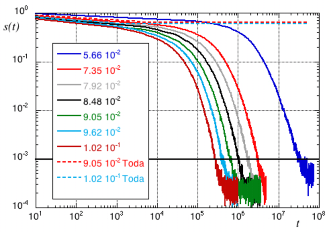
Figure 1: Entropy $s(t)$ as a function of time for different simulations of the $\alpha$-FPU system characterized by different values of $\epsilon$. In the plot two simulations of the Toda lattice are also presented. A horizontal line at $s=0.001$ is also included as a threshold for estimating the equipartition time.

A main result of this study is that the $\alpha$-FPU model should reach thermal equilibrium on a time scale of $1/\epsilon^{8}$ for arbitrary small nonlinearity. Therefore, we use numerical simulations to support our theoretical finding. We integrate in time equation (2) with $N=32$ particles and with $m=\gamma=1$ by using the sixth order symplectic integrator scheme described in [35]. Different values of $\epsilon$ have been considered between $0.0566$ and $0.11$; due to the slow time needed to reach thermalization, computations become soon prohibitive for smaller values of $\epsilon$.

We emphasize that the thermal equilibrium is a statistical concept, therefore averages should be taken to observe it. It may be possible to average over time, as in many previous simulations of the FPU model. We find such approach to be problematic, because often the time window used is of the same order of the characteristic time to reach equipartition of energy. We have chosen to perform ensemble averaging, typically over 1000 realizations (some convergence tests have also been made over 2000 ensembles). Two types of initial conditions have been considered: in the first one, we have initialized only the modes $k=\pm 1$; in the second one, initial conditions are characterized by constant energy only over the modes $k=\pm 1,\pm 2,\pm 3,\pm 4,\pm 5$. Different random phases are then applied to the Fourier amplitudes for each realization.

As in [33], we have introduced, as an indicator of thermalization, the following entropy:

$$s(t)=\sum\limits_{k}f_{k}\log f_{k}$$ (27)

with

$$f_{k}=\frac{N-1}{E_{tot}}\omega_{k}\langle|a_{k}|^{2}\rangle,\;\;\;E_{tot}=\sum\limits_{k}{\omega_{k}\langle|a_{k}|^{2}\rangle}$$ (28)

and $\langle...\rangle$ defines the average over the realizations. We have used in the definition $N-1$ instead of $N$, because, with periodic boundary conditions, the modes that thermalize are $N-1$ and not $N$ (the first mode $k=0$ is not involved in the dynamics). For a thermalized spectrum, the value of the entropy is theoretically 0. Through our numerical simulations, we have reached a minimum value of $s$ very close to $10^{-4}$. In figure 1 we show the evolution of the entropy for different values of $\epsilon$. As one can observe, in the large time limit, the entropy reaches very small values. Two typical simulations of the Toda lattice are also included in the figure and show that, as expected, no thermalization is reached. Just as an example, we show in Figure 2 the energy spectrum, defined as $E(k)=\omega_{k}\langle|a_{k}|^{2}\rangle$, at different time steps for the simulation with $\epsilon=0.0848$. The spectrum is normalized by $(N-1)/E_{tot}$ in such a way that, once thermalization has been reached, all values of the energy are around 1.

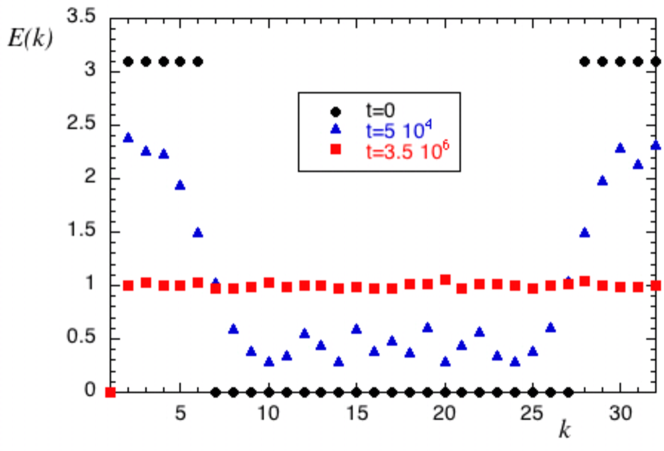
Figure 2: Energy spectrum at different time steps from numerical simulations of the $\alpha$-FPU system. Black dots correspond to the initial condition; blue triangles correspond to an intermediate stage and red squares to the final thermalized spectrum. Note that energy is presented in linear scale.

In order to verify the expected time scaling, we introduced an entropy threshold $s_{thr}$ to estimate the time it takes for the system to reach thermodynamic equilibrium. Specifically, we have defined $t_{eq}$ as the time in which the entropy $s$ reaches the value of $s_{thr}=0.001$ (see an horizontal line at $s=0.001$ in Figure 1). We present in Figure 3 the log-log plot of this time $t_{eq}$ as a function of $\epsilon$ for the two types of simulations considered. Figure 3 also shows the straight line with slope -8. All the points are pretty much aligned with this straight line. This numerical result is consistent with our analytic prediction that time $t_{eq}$ is proportional to $\epsilon^{-8}$.

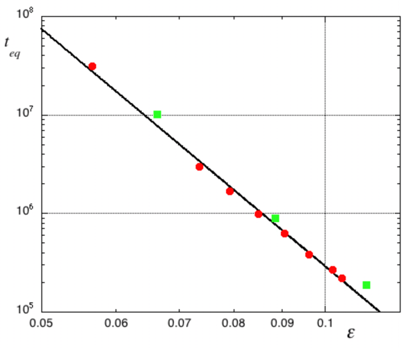
Figure 3: Equilibrium time $t_{eq}$ as a function of $\epsilon$ in Log-Log coordinates. Red dots represent numerical experiments of the $\alpha$-FPU system with broad band initial conditions, i.e. modes $k=\pm 1,\pm 2\pm 3,\pm 4,\pm 5$ have been initially perturbed; green dots represent narrow band initial conditions, i.e. modes $k=\pm 1$ have been initially perturbed. The straight line corresponds to power law of the type $1/\epsilon^{8}$

The last check on the validity of the theory, free of an arbitrary threshold, is made by rescaling the time evolution of the entropy: in Figure 4 we show the evolution of the entropy as a function of $\epsilon^{8}t$ for different values of $\epsilon$. As predicted by the theory, the curves seem to collapse to a single one.

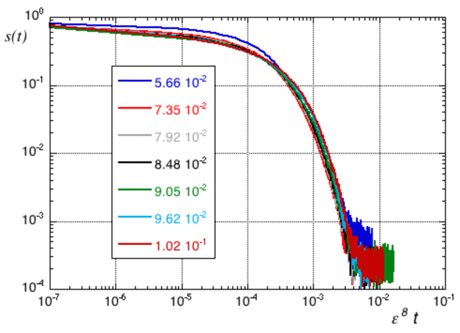
Figure 4: Entropy $s(t)$ as a function of $\epsilon^{8}t$ for different simulations of the $\alpha$-FPU system characterized by different values of $\epsilon$.

7 A note on the thermodynamic limit

In statistical mechanics one is usually interested in the thermodynamic limit. Assuming that the length of the chain is $L$ and the spacing between masses is $\Delta x$, we let $N\rightarrow\infty$ and $L\rightarrow\infty$ in such a way that $\Delta x=L/N=const$. Wave numbers in Fourier space become dense, $\Delta k=2\pi/L\rightarrow 0$. The dispersion relation now becomes $\omega(\kappa)=2\left|\sin(\kappa/2)\right|$, where we have set $\Delta x=1$ and $\kappa=k\Delta k$. Assuming that $\kappa\in\mathbb{R}$, the same approach based on resonant interactions can now be performed. It turns out that four wave, non-isolated, resonant interactions exist. An example is provided by the following two connected quartets:

$$\begin{split}(-0.05710747907971836...,1.604305030276316...,1/2,\pi/3)\\ (-0.12747695473542747...,2.198273281530324...,1/2,\pi/2),\end{split}$$

that can be found numerically using the resonant conditions (19). The existence of interconnected resonant quartets implies that in the thermodynamic limit the equipartition may be achieved by resonant four wave interactions; in this case the system is completely described by the traditional wave turbulence four-wave kinetic equation [11]. The time scale of the resonant four wave kinetic equation is given by the $1/\epsilon^{4}$, much shorter than $1/\epsilon^{8}$, i.e. the time scale of equipartition for a system of $N$=16,32,64 masses.

8 A short discussion on other possible scenarios

The FPU system has been the subject of many studies and a presentation of all the different points of view developed in sixty years is merely impossible. However, here we briefly present some routes to equipartition that are accepted nowadays in the literature.

In the pioneering work of Izrailev and Chirikov [31], the idea that an initial energy larger than a critical value is needed in order to reach thermalization was put forward. Such concept is based on the fact that the nonlinearity changes the linear dispersion relation and, consequently, the resonant condition in frequency is then modified. When the nonlinearity becomes large enough, a mechanism of “overlap of frequencies” may take place. Such phenomenon lead to the introduction of the so called “stochastic threshold”. In the late sixties, not everybody shared such an idea; indeed, for example in 1970 Ford and Lunsford [32] insisted on the fact that mixing could be observed also in the limit as the nonlinearity goes to zero.

In favor of the existence of a threshold, a large number of papers have been written and different scenarios have been presented, see for example [33]. A very interesting picture has been presented in [34]: the authors considered the $\beta$-FPU system with initial conditions characterized by the highest mode (also known as the $\pi$-mode). They showed that, above an energy threshold which can be computed analytically, the $\pi$ mode is modulationally unstable and give rise to localized chaotic structures (breathers). They related the lifetime of the chaotic breathers to the time necessary for the system to reach equipartition. This interesting scenario cannot be directly applied to the $\alpha$-FPU; the reason is that a straightforward calculation shows that a single mode in the $\alpha$-FPU is modulationally stable. This does not imply that in the $\alpha$-FPU model localized coherent structure do not exist. Indeed, being the system close to the Korteweg de Vries equation, solitary waves may be excited, if the initial energy is sufficiently large. However, our main finding is that such strong nonlinearity is not needed to reach equipartition. Our explanation is based only on resonant interactions and, as a result, equipartition can take place for arbitrary small nonlinearity, as confirmed by numerical simulations.

We mention once more that our analyses are based on $N$=$16$ or $32$ or $64$ masses, as the original simulations of Fermi, Pasta and Ulam; by changing the number of masses the solution to the resonant conditions may change; therefore, each case should be treated separately and possibly different scenarios may appear, as for example the thermodynamic limit described above.

9 Conclusion

$i)$ Resonant triads are forbidden; this implies that, on a short time scale, three-wave interaction will generate a reversible dynamics. This is what has been observed originally by Fermi, Pasta and Ulam and what is known as metastable state (see for example [4]).
$ii)$ A suitable canonical transformation allows us to look at higher order interactions in the system which are responsible for longer time scale dynamics.
$iii)$ Four-wave resonant interactions exist; however, we have shown that for $N$=16,32,64 each resonant quartet is isolated, preventing the full spread of the energy across the spectrum and thermalization.
$iv)$ Six wave interactions lead to irreversible energy mixing.
$v)$ The time scale of equipartition in a weakly nonlinear random system described by $\alpha$-FPU system is $1/\epsilon^{8}$. The result is consistent with our numerical simulations.
$vi)$ In the thermodynamic limit, non-isolated resonant quartets exits and the time scale of equipartition is $1/\epsilon^{4}$.

- [1] E. Fermi, J. Pasta, and S. Ulam. Studies of nonlinear problems. No. LA 1940. I, Los Alamos Scientific Laboratory Report No. LA-1940, 1955.
- [2] Zakharov, V. E., and Schulman, E. I. (1991). Integrability of nonlinear systems and perturbation theory. In What Is Integrability? (pp. 185-250). Springer Berlin Heidelberg.
- [3] Zabusky, N. J., and Kruskal, M. D. (1965). Interaction of” Solitrons” in a Collisionless Plasma and the Recurrence of Initial State. Princeton University Plasma Physics Laboratory.
- [4] Benettin, G., Christodoulidi, H., and Ponno, A. (2013). The Fermi-Pasta-Ulam Problem and Its Underlying Integrable Dynamics. Journal of Statistical Physics, 1-18.
- [5] Ford, J. (1992). The Fermi-Pasta-Ulam problem: paradox turns discovery. Physics Reports, 213(5), 271-310.
- [6] Weissert, T. P. (1999). The genesis of simulation in dynamics: pursuing the Fermi-Pasta-Ulam problem. Springer-Verlag New York, Inc..
- [7] Berman, G. P., and Izrailev, F. M. (2005). The Fermi-Pasta-Ulam problem: fifty years of progress. Chaos (Woodbury, NY), 15(1), 15104.
- [8] Carati, A., Galgani, L., and Giorgilli, A. (2005). The Fermi Pasta Ulam problem as a challenge for the foundations of physics. Chaos: An Interdisciplinary Journal of Nonlinear Science, 15(1), 015105-015105.
- [9] Gallavotti, G. (Ed.). (2008). The Fermi-Pasta-Ulam problem: a status report (Vol. 728). Springer.
- [10] Jackson, E. A.(1978). Nonlinearity and irreversibility in lattice dynamics. Rocky Mountain J. Math, 8,27-196.
- [11] Zakharov, V. E., L’vov, V. S., and Falkovich, G. (1992). Kolmogorov spectra of turbulence 1. Wave turbulence. Kolmogorov spectra of turbulence 1. Wave turbulence., by Zakharov, VE; L’vov, VS; Falkovich, G.. Springer, Berlin (Germany), 1992, 275 p., ISBN 3-540-54533-6, 1.
- [12] Nazarenko, S. (2011). Wave turbulence (Vol. 825). Springer.
- [13] Papa, E., and MacDonald, A. H. (2005). Edge state tunneling in a split Hall bar model. Physical Review B, 72(4), 045324.
- [14] Whitham, G. B. (2011). Linear and nonlinear waves (Vol. 42). John Wiley and Sons.
- [15] Arnol’d, V. I. (1963). Small denominators and problems of stability of motion in classical and celestial mechanics. Russian Mathematical Surveys, 18(6), 85-191.
- [16] Krasitskii, V. P. (1994). On reduced equations in the Hamiltonian theory of weakly nonlinear surface waves. Journal of Fluid Mechanics, 272(1).
- [17] Dyachenko, A. I., Lvov, Y. V., and Zakharov, V. E. (1995). Five-wave interaction on the surface of deep fluid. Physica D: Nonlinear Phenomena, 87(1), 233-261.
- [18] Janssen, P. (2004). The interaction of ocean waves and wind. Cambridge University Press
- [19] Janssen, P. A., and Onorato, M. (2007). The intermediate water depth limit of the Zakharov equation and consequences for wave prediction. Journal of Physical Oceanography, 37(10), 2389-2400.
- [20] Zakharov, V. E. (1968). Stability of periodic waves of finite amplitude on the surface of a deep fluid. Journal of Applied Mechanics and Technical Physics, 9(2), 190-194.
- [21] Henrici, A., and Kappeler T.. ”Results on normal forms for FPU chains.” Communications in Mathematical Physics 278.1 (2008): 145-177.
- [22] Rink, B. (2006). Proof of Nishida’s conjecture on anharmonic lattices. Communications in mathematical physics, 261(3), 613-627.
- [23] Gershgorin, B., Lvov, Y. V., and Cai, D. (2007). Interactions of renormalized waves in thermalized Fermi-Pasta-Ulam chains. Physical Review E, 75(4), 046603.
- [24] Dyachenko, A. I., Kachulin, D. I., and Zakharov, V. E. E. (2013). On the nonintegrability of the free surface hydrodynamics. JETP letters, 98(1), 43-47.
- [25] Toda, M. (1967). Vibration of a chain with nonlinear interaction. Journal of the Physical Society of Japan, 22(2), 431-436.
- [26] Ferguson Jr, W. E., Flaschka, H., and McLaughlin, D. W. (1982). Nonlinear normal modes for the Toda chain. Journal of Computational Physics, 45(2), 157-209.
- [27] Casetti, L., Cerruti-Sola, M., Pettini, M., and Cohen, E. G. D. (1997). The Fermi-Pasta-Ulam problem revisited: stochasticity thresholds in nonlinear Hamiltonian systems. Physical Review E, 55(6), 6566.
- [28] Zakharov, V. E., and Schulman, E. I. (1988). On additional motion invariants of classical Hamiltonian wave systems. Physica D: Nonlinear Phenomena, 29(3), 283-320.
- [29] Ponno, A., Christodoulidi, H., Skokos, C., and Flach, S. (2011). The two-stage dynamics in the Fermi-Pasta-Ulam problem: from regular to diffusive behavior. Chaos: An Interdisciplinary Journal of Nonlinear Science, 21(4), 043127-043127.
- [30] Hemmer, P. C. (1959). Dynamic and stochastic types of motion in the linear chain. Tapir forlag.
- [31] Izrailev, F. M., and Chirikov, B. V. (1966, July). Statistical properties of a nonlinear string. In Sov. Phys. Dokl (Vol. 11, No. 1, pp. 30-32).
- [32] Ford, J., and Lunsford, G. H. (1970). Stochastic behavior of resonant nearly linear oscillator systems in the limit of zero nonlinear coupling. Physical Review A, 1(1), 59.
- [33] Livi, R., Pettini, M., Ruffo, S., Sparpaglione, M., and Vulpiani, A. (1985). Equipartition threshold in nonlinear large Hamiltonian systems: The Fermi-Pasta-Ulam model. Physical Review A, 31(2), 1039.
- [34] T. Cretegny, T. Dauxois, S. Ruffo, and A. Torcini, (1998). Localization and equipartition of energy in the -FPU chain: Chaotic breathers. Physica D: Nonlinear Phenomena, 121, 109.
- [35] Yoshida, H. (1990). Construction of higher order symplectic integrators. Physics Letters A, 150(5), 262-268.