TEMPERATURE EVOLUTION OF MAGNETIC FLUX ROPE IN A FAILED SOLAR ERUPTION

Abstract

In this paper, we report for the first time the detailed temperature evolution process of the magnetic flux rope in a failed solar eruption. Occurred on January 05, 2013, the flux rope was impulsively accelerated to a speed of $\sim$400 km/s in the first minute, then decelerated and came to a complete stop in two minutes. The failed eruption resulted in a large-size high-lying ($\sim$100 Mm above the surface) high-temperature “fire ball” sitting in the corona for more than two hours. The time evolution of the thermal structure of the flux rope was revealed through the differential emission measure analysis technique, which produced temperature maps using observations of the Atmospheric Imaging Assembly on board Solar Dynamic Observatory. The average temperature of the flux rope steadily increased from $\sim$5 MK to $\sim$10 MK during the first nine minutes of the evolution, which was much longer than the rise time (about three minutes) of the associated soft X-ray flare. We suggest that the flux rope be heated by the energy release of the continuing magnetic reconnection, different from the heating of the low-lying flare loops, which is mainly produced by the chromospheric plasma evaporation. The loop arcade overlying the flux rope was pushed up by $\sim$10 Mm during the attempted eruption. The pattern of the velocity variation of the loop arcade strongly suggests that the failure of the eruption be caused by the strapping effect of the overlying loop arcade.

1 INTRODUCTION

Magnetic flux ropes play an important role in solar eruptions manifested as coronal mass ejections (CMEs) and/or flares. Recently, a new line of observational structures, namely EUV hot-blobs and/or channels, have been proposed to be the most direct manifestation of flux ropes (Cheng et al. 2011; Zhang et al. 2012; Cheng et al. 2013; Patsourakos et al. 2013) with the Atmospheric Image Assembly (AIA; Lemen et al. 2012) on board the Solar Dynamics Observatory (SDO) (Pesnell et al. 2012). In particular, Zhang et al. (2012) revealed the flux rope as a conspicuous hot channel structure prior to and during a solar eruption, which initially appeared as a writhed sigmoid with a temperature as high as $\sim$10 MK, then continuously transformed itself toward a semi-circular shape and acted as the essential driver of the resulting CME.

While previous studies have been focusing on the morphological and kinematic evolution of magnetic flux ropes, little is known about their thermal evolution. The scenario of heating solar flare loops is well accepted in classical flare models (Carmichael 1964; Sturrock 1966; Hirayama 1974; Kopp & Pneuman 1976), in which flare loops are mainly heated by the thermal plasma from the chromospheric evaporation (Doschek et al. 1980; Feldman et al. 1980). Now the question is whether flux ropes, seen as expanding hot channels in a much higher corona, are heated by the same process. In this letter, we intend to use differential-emission-measure (DEM) based temperature analysis method on an event of failed flux rope eruption to address this issue. Recently, DEM analyses have been applied to diagnose the physical properties of CMEs (Zhukov & Auchère 2004; Landi et al. 2010; Tian et al. 2012; Cheng et al. 2012; Tripathi et al. 2013), the quiet Sun (Vásquez et al. 2010) and the post-flare loop systems (Reeves & Weber 2009; Warren et al. 2013). The multi-passband broad-temperature capability of AIA makes it ideal for constructing DEM models. We find that this method is particularly useful in studying the failed solar eruption, in which the thermal structure is conspicuous and long lasting in AIA field of view (FOV).

There have been several studies on failed eruptions, but the physical cause of the failure remains elusive. It is found that long duration flares tend to be more eruptive (Kahler et al. 1989), but many other factors could be invovled, such as the interaction between filaments and their associated magnetic environment (Ji et al. 2003; Williams et al. 2005; Gibson & Fan 2006; Jiang et al. 2009; Kuridze et al. 2013), the degree of the helical twist in the filament (Rust & LaBonte 2005), the overlying arcade field (Wang & Zhang 2007), and the position of the reconnection site (Gilbert et al. 2007). Numerical simulations showed that the kink instability could trigger a failed filament eruption if the overlying magnetic field decreases slowly with height (e.g., Török & Kliem, 2005).

For the failed eruption in this paper, we can clearly observe and track the flux rope structure, as a hot EUV blob, before, during and after the eruption. Using advanced DEM-based temperature map method, we reveal, for the first time, the detailed thermal evolution of the flux rope, and conclude that the thermal structure is caused by the direct heating from the energy release of the magnetic reconnection in the flux rope. Further, we find convincing evidences that the failure of the eruption is caused by the strapping effect of the overlying magnetic loop arcade. In Section 2, we present the observations and results, which are followed by a summary and discussions in Section 3.

2 OBSERVATIONS AND RESULTS

2.1 Instrument and Method

The AIA images the multi-layered solar atmosphere through 10 narrow UV and EUV passbands almost simultaneously with high cadence (12 seconds), high spatial resolution (1.2 arcseconds) and large FOV (1.3 R_⊙). The temperature response functions of their passbands indicate an effective temperature coverage from 0.6 to 20 MK (O’Dwyer et al. 2010; Del Zanna et al. 2011; Lemen et al. 2012;). During eruptions, the 131 Å and 94 Å passbands are more sensitive to the hot plasma from flux ropes and flare loops, while the other passbands are better at viewing the cooler leading front and dimming regions (e.g., Cheng et al. 2011; Zhang et al. 2012).

The observed flux $F_{i}$ for each passband can be determined by

$$F_{i}=\int R_{i}(T)\times DEM(T)dT$$

where the $R_{i}(T)$ and $DEM(T)$ are the temperature response function of passband $i$ and the plasma DEM in the corona, respectively. Cheng et al (2012) and we use the “xrt_dem_iterative2.pro” routine in SSW package to compute the DEM. This code was originally designed for Hinode$/$X-ray Telescope data (Golub et al. 2004; Weber et al. 2004) and was modified slightly to work with AIA data (Schmelz et al. 2010, 2011a, 2011b; Winebarger et al. 2011; Cheng et al. 2012). More details and tests of this method were discussed in the Appendix of Cheng et al. (2012). Here, we use the DEM-weighted average temperature per pixel defined in the following formula (Cheng et al. 2012) to construct the temperature map in spatial domain and study their temperature evolution in time.

$$\overline{T}=\frac{\int DEM(T)\times TdT}{\int DEM(T)dT}$$

Errors in DEM inversion arise from the uncertainties in the response function $R_{i}(T)$ (Judge 2010) and the background determination (e.g., Aschwanden & Boerner 2011). According to Cheng et al. (2012), the error of DEM-weighted temperature at the flux rope center could be $\sim$15%. We should point out that the plasma, integrated along the line of sight, contains multiple temperatures. The “weighted” temperature we are obtaining here, is an indicator of the overall thermal trend of the plasma in the temperature range the instrument is sensitive to.

2.2 The Event and Its Temperature Evolution

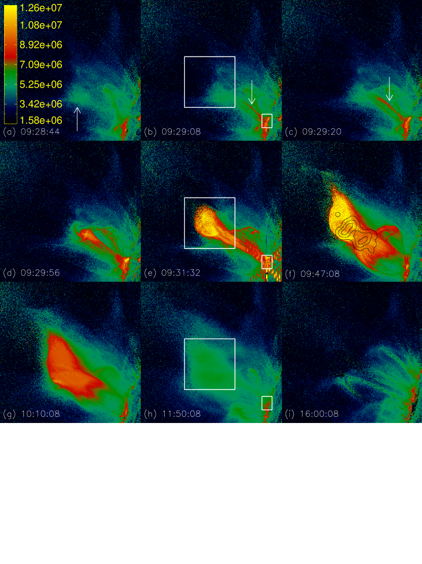
Figure 2: Temperature evolution process of the failed flux rope eruption. The FOV is the same as in Figure 1. (Animations of the full evolution of the temperature maps and a color version of this figure are available in the online journal.)

On 2013 January 5, an M1.7 class soft X-ray flare occurred at the northeast limb of the Sun, which started at 09:28 UT and peaked at 09:31 UT. The flare was located at $\sim$N20E88 (NOAA 11652) from the perspective of the Earth. No associated CME was observed by the Large Angle Spectroscopic Coronagraph (LASCO; Brueckner et al. 1995) and the Sun Earth Connection Coronal and Heliospheric Investigation (SECCHI; Howard et al. 2008). But in AIA 131 Å and 94 Å passbands, an obvious structure with high temperature was observed to erupt, but stopped to rise further. In Figure 1, we present the observations of this failed eruption process. Panels (a)-(c) are observations from 131 Å , (d) is a composite image of 94 Å (Blue channel) and 171 Å (Green channel) and (e)-(f) are composite images of 131 Å (Red channel) and 171 Å . (See supplementary Movies 1 and 2 for the entire and continuous eruption process in six AIA EUV passbands). The left panels show the coronal images immediately before the eruption. The upper-pointing red arrows indicate the position of the flux rope structure that was about to rise and erupt. The flux rope is better seen in 94 Å in the early time of the evolution, which means that its initial temperature should be around 6 MK; this is consistent with the DEM analysis result shown in Figure 2 (a). This temperature effect explains why the flux rope is better seen in 94 Å  but less visible in 131 Å (Figure 1 (a)) and completely invisible in 171 Å (Figure 1(d)) in the early time. This flux rope can be observed for its favorable orientation. It seems that the axis of the rope lied along the line of sight at the limb of the Sun, making it a bright blob-like structure. At 09:28:56, a hot and fast narrow jet started to appear in 131 Å images, and became obvious at 09:29:20 as depicted with blue arrows in Figures 1(b) and (e). With DEM analysis, we learned that the hot jet temperature is around 8 MK (Figures 2(b) and (c)). Therefore, the jet is better seen in 131 Å  but could not be observed in 171 Å passband, see Figure 1(e).

The flux rope started to rise at about 09:29:20 UT, stopped at 09:32:35 UT, and then stayed in the position for several hours before faded away. The flux rope could not be observed in 171 Å during the entire process because of its high temperature. But the 171 Å observations show the movement of the overlying loop arcade clearly (bottom panels in Figure 1). The asterisks in the panels show the position of the inner edge of the overlying loop arcade. With a horizontal white line passing through the two asterisks in the frames of earlier times when the loop arcade had not begun to rise, it is easy to notice that the loop arcade was shifted and raised to a higher position following the eruption. The 211 Å and 193 Å observations also show the overlying loops stressed by the rope (See supplementary Movie 1). The red plus symbols shown in the right panels point to the apex position of the flux rope.

Figure 2 shows a sequence of temperature maps throughout the entire thermal evolution process of the event. Before the eruption, the temperature of the flux rope (depicted with a white arrow) is over 5 MK as shown in Figure 2(a). Figures 2(b) and (c) show the hot jet (depicted with the white arrows) underneath the flux rope. The appearance of the hot jet seemed to signal the onset of the flare and also the onset of the flux rope rising. We find that the temperature over the eruption region increased quickly (See supplementary movie 3). Two sub-regions, as depicted with a large square in the high corona and a small rectangle close to the solar surface in Figures 2(b), (e) and (h), are selected to be the regions of the flux rope and flare loops respectively, for the purpose of tracking their temperature evolutions. To obtain the characteristic average temperature of the entire flux rope, all the pixels with temperatures greater than 5.0 MK in the selected square are regarded as the flux rope pixels, and their average temperature is regarded as the characteristic temperature. The same way is used to get the average temperature of the flare loop region as selected with the rectangle.

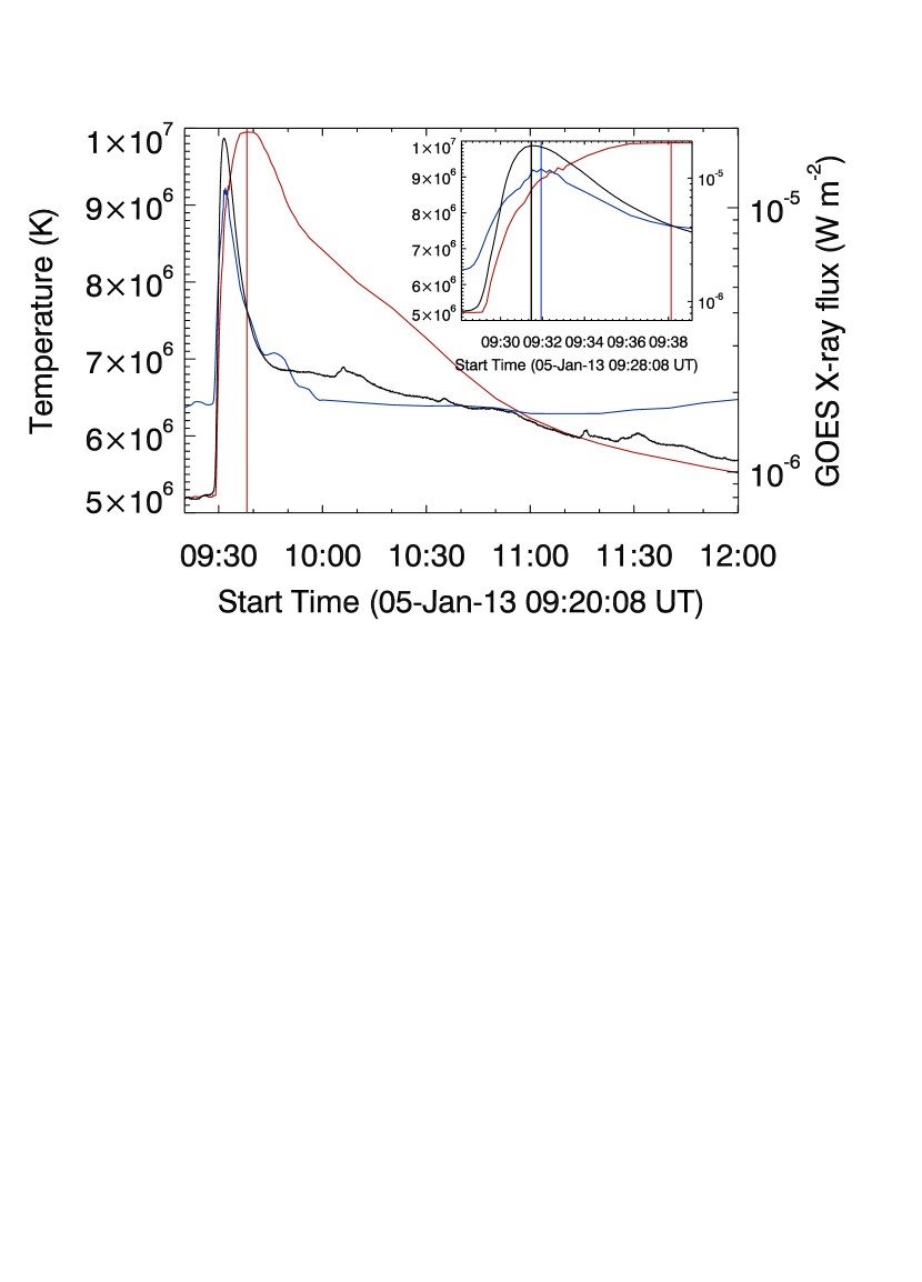
Figure 3: The temperature-time profiles of the high-lying flux rope (red) and the low-lying flare loops (blue), along with the profile of GOES soft X-ray 1-8 Åflux (black). (A color version of this figure is available in the online journal.)

The temperature evolution of the flux rope and the flare loops are shown in Figure 3 with red and blue solid line, respectively, along with the Geostationary Operational Environmental Satellite (GOES) soft X-ray 1-8 Å profile in the black line. The insert panel in Figure 3 is an enlarged portion from 09:28:08 to 09:39:08 UT to better show the relations at the beginning of the eruption. Apparently, the temperature profile of the flare loops is almost the same as the soft X-ray profile, i.e., the same peak time and the similar rise phase. This is consistent with the classic thick-target model that the flare region is heated by the precipitation of energetic electrons accelerated in flare reconnection; Note that we might under-estimate the temperature of the flare loops for the following two reasons: first, a part of the hot near-footpoint sources might be occulted by the limb; second, a small fraction of the flare region were saturated in AIA images. Nevertheless, we don’t believe that these effects will change the temporal profile of the temperature evolution. However, the temperature evolution of the flux rope is remarkably different from that of the flare loops, i.e., the duration of the temperature increase lasted much longer than that in the flare loops and the rise phase of the soft X-ray flare. For clarity of discussion, we may divide this duration into two phases: impulsive-heating phase and post-impulsive-heating phase. In the impulsive-heating phase, the temperature increased from $\sim$5.2MK ($\sim$09:29 UT) to $\sim$8.5 MK ($\sim$09:31 UT), while the temperature increased from $\sim$8.5 MK to $\sim$10 MK ($\sim$09:38 UT) during the post-impulsive-heating phase. Then the temperature began to slowly decrease to $\sim$5.6 MK until 12:00 UT. It is obvious that the impulsive and post-impulsive heating phases correspond well with the rise phase and decay phase of the associated flare.

The continuing rise of temperature in the flux rope after the flare rise phase is an interesting discovery in this study. It seems that the heating of the flux rope should be different from that of the flare loops. We suggest that the direct thermal heating from the magnetic reconnection region, without via the chromospheric evaporation, should be responsible for the heating of the flux rope. The continuing strong heating of the flux rope after the flare soft X-ray peak time is related with the continuing energy release during the decay phase of the soft X-ray flare. In this long duration flare, there should be continuing magnetic reconnection in the corona. Further, the failure of the eruption resulted in less energy converted to the kinetic energy of the bulk plasma from the released magnetic energy; this extra energy should further heat the flux rope trapped in the corona. Consequently, the eruption produced a conspicuous large-size high-lying ($\sim$100 Mm above the surface) high-temperature ($\sim$6–10 Mk) “fire ball” sitting in the corona for more than two hours. In the end, the hot structure faded away and became indistinguishable from the ambient as shown in Figure 2(i).

To further elucidate the relation between the flux rope heating and the magnetic reconnection, we investigated the location of the coronal hard X-ray sources using data from Reuven Ramaty High Energy Solar Spectroscopic Imager (RHESSI) (Lin et al 2002). Unfortunately, RHESSI was in night until $\sim$09:46 UT. RHESSI observations around 09:47 UT are thus selected and shown as black contours in the 12–20 keV band at 50%, 70% and 90% of the maximum in Figures 1(c) and 2(f). The contours apparently show a double X-ray source. It has been suggested that the region of magnetic reconnection should be between the two X-ray sources (e.g., Liu et al. 2008). Therefore, it seems that the magnetic reconnection separates the flux rope structure into two parts: the upper part and the lower part. Such scenario of magnetic reconnection leading to partial eruption have been reported in several studies (Gilbert et al. 2000; Gibson & Fan 2006; Tripathi et al. 2007; Sterling et al. 2011; Tripathi et al. 2013).

2.3 Kinematic Evolution of The Failed Eruption

We also study the kinematic evolution process of the flux rope and its overlying loops. The heights of flux rope apexes (red plus symbols shown in the right panels of Figure 1) and the inner edge of the overlying loop arcades (blue asterisk symbols shown in the bottom panels of Figure 1) are tracked in the AIA images and shown in Figure 4(a). Their velocities are shown in Figure 4(b), along with the GOES soft X-ray 1-8 Å profile shown in the black line. The velocities are calculated from the numerical differentiation using the 3-point Lagrangian interpolation of the height-time data. Note that the uncertainties of the velocities come mainly from the uncertainties in the height measurement. The measurement errors are estimated to be 2 pixels. These errors are propagated in the standard way to estimate the errors of velocity. The red, blue and black filled circles show the times of the maximum velocities of the flux rope and overlying loops, and the peak of the soft X-ray flux, respectively.

From Figure 4(a) we find that the flux rope started to show noticeable movement at 09:29:20 UT, and the loop arcade, started to move at a later time at 09:30:11 UT. Apparently, the ascending motion of the overlying loop arcade is induced by the rising motion of the erupting flux rope; the early interaction between the flux rope and the loop arcade should take place at a time between 09:30:11 UT and 09:30:23 UT as indicated by the two vertical dashed lines in Figure 4; at this time, the flux rope had already obtained a speed of about 400 km/s. The interaction apparently prevented the further eruption of the flux rope and led its velocity to decrease quickly, until came to a full stop two minutes later. Before the contact of the interaction, the velocity of the flux rope increased from $\sim$95 km s^-1 at 09:39:20 UT to $\sim$431 km s^-1 at 09:30:08 UT; during this 48 s of “free” acceleration, the average acceleration rate is estimated to be $\sim$7000 m s^-2. This is an extremely strong acceleration, when compared with the rates of most CMEs which are typically lower than 1000 m s^-2 (Zhang & Dere 2006). The interaction made the velocity of the rope just increased from 431 km s^-1 at 09:30:08 UT to 438 km s^-1 at 09:30:20 UT with an average acceleration 580 m s^-2. Then the velocities of the flux rope began to decrease quickly from 438 km s^-1 to almost zero at 09:32:35 UT with the average decceleration rate 3240 m s^-2. On the other hand, the velocity of the loop arcade started at about 70 km s^-1 when the movement became noticeable at 09:30:11 UT, and increased to 98 km s^-1 at 09:30:23 UT as its peak value. The early acceleration of the loop arcade was not observed, probably because the early interaction was short and prompt, even the 12-second cadence of AIA was not sufficient to capture the evolution. The instantaneously accelerated loop arcade immediately began its deceleration. The deceleration phase of the loop arcade coincided well with that of the flux rope, coming to a full stop about two minutes later. We conclude that the magnetic strapping effect of the overlying loop arcade, likely due to the magnetic tension force along the loops, made the eruption a failed one, instead of forming an escaping CME.

3 SUMMARY AND DISCUSSIONS

A failed flux rope eruption associated with an M1.7 class flare was observed by the AIA at the northeast limb of the Sun on 2013 January 5, which provided us an unprecedented opportunity for studying the detailed temperature evolution of the flux rope. We find that the flux rope existed in the corona with a high temperature ($\sim$5 MK) before its eruption. The temperature evolution of the flux rope can be divided into two phases: impulsive-heating phase and post-impulsive-heating phase, which correspond well with the rise phase and decay phase of the associated flare. On the contrary, the temperature of the low-lying flare loops only increased during the flare rise phase, and quickly decreased during the decay phase. Furthermore, there was a gap of low temperature between the flux rope and the flare loops. All of these observations indicate that the flux rope should be heated by a different process from that of the flare loops. The heating process of flare loops have been well understood and widely accepted as summarized below. Energetic electrons and ions produced by flare magnetic reconnection precipitate from the coronal acceleration site and lose their energy in the dense underlying chromosphere via Coulomb collisions. The temperature in the chromosphere increases and the resulting pressure exceeds the ambient chromospheric pressure, which leads the heated plasma to expand along the magnetic field, forming flare loops (Doschek et al. 1980; Feldman et al. 1980). While for the flux rope, we suggest that it should be heated directly by the thermal energy generated at the reconnection site through the thermal conduction. It is unlikely that chromospheric evaporation plays a strong role in heating the flux rope.

The velocity analysis of the flux rope and the overlying loop arcades strongly suggests that the failure of the eruption be caused by the strapping effect of the overlying magnetic loop arcade. The strapping effect, or the tension force of the line-tying field, is the determining factor that contained the flux rope from further eruption.

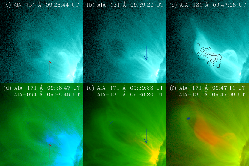
Figure 1: The failed flux rope eruption on 2013 January 5. The FOV is taken to be [-1140,-890] and [320, 570] arcsec for the horizontal and vertical axis, respectively. (Animations of the eruption process with full AIA cadence and a color version of this figure are available in the online journal)

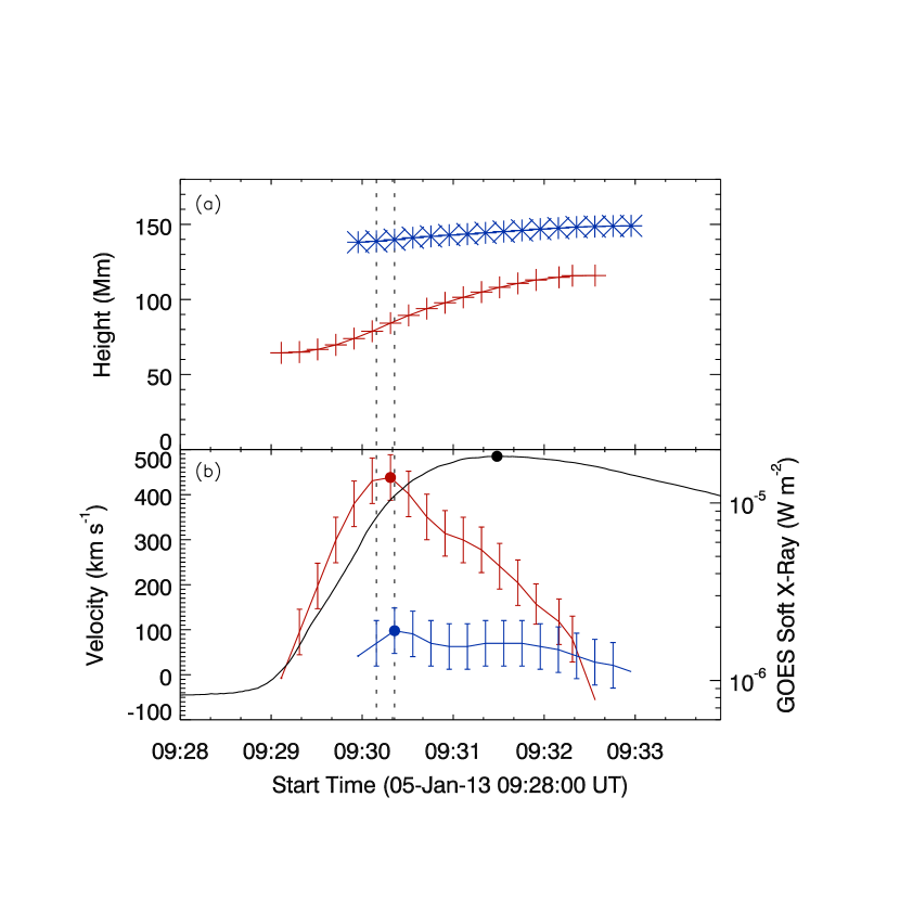
Figure 4: (a) The height-time profiles of the flux rope (red) and the loop arcade (blue). (b) The velocity-time profiles of the flux rope (red) and the loop arcade (blue), along with the profile of GOES soft X-ray 1-8 Åflux. (A color version of this figure is available in the online journal.)

References

- Aschwanden & Boerner (2011) Aschwanden, M. J., & Boerner, P. 2011, ApJ, 732, 81
- Brueckner et al. (1995) Brueckner, G. E., Howard, R. A., Koomen, M. J., et al. 1995, Sol. Phys., 162, 357
- Carmichael (1964) Carmichael, H. 1964, in NASA Special Publication 50, The Physics of Solar Flares, ed. W. N. Hess (Washington, DC: NASA), 451
- Cheng et al. (2013) Cheng, X., Zhang, J., Ding, M. D., et al. 2013, ApJ, 769, L25
- Cheng et al. (2011) Cheng, X., Zhang, J., Liu, Y., & Ding, M. D. 2011, ApJ, 732, L25
- Cheng et al. (2012) Cheng, X., Zhang, J, Saar, S. H., & Ding, M. D. 2012, ApJ, 761, 62
- Del Zanna et al. (2011) Del Zanna, G., O’Dwyer, B., & Mason, H. E. 2011, A&A, 535, A46.
- Doschek et al. (1980) Doschek, G. A., Feldman, U., Kreplin, R. W., & Cohen, L. 1980, ApJ, 239, 725
- Feldman et al. (1980) Feldman, U., Doschek, G. A., Kreplin, R. W., & Mariska, J. T. 1980, ApJ, 241, 1175
- Gibson & Fan (2006) Gibson, S. E., & Fan, Y. 2006, ApJ, 637, L65
- Gilbert et al. (2007) Gilbert, H. R., Alexander, D., & Liu, R. 2007, Sol. Phys., 245, 287
- Gilbert et al. (2000) Gilbert, H. R., Holzer, T. E., Burkepile, J. T., & Hundhausen, A. J. 2000, ApJ, 537, 503
- Golub et al. (2004) Golub, L., Deluca, E. E., Sette, A., & Weber, M. 2004, in ASP Conf. Ser. 325, The Solar-B Mission and the Forefront of Solar Physics, ed. T. Sakurai & T. Sekii (San Francisco, CA: ASP), 217
- Hirayama (1974) Hirayama, T. 1974, Sol. Phys., 34, 323
- Howard et al. (2008) Howard, R. A., Moses, J. D., Vourlidas, A., et al. 2008, Space Sci. Rev., 136, 67
- Ji et al. (2003) Ji, H. S, Wang, H. M., Schmahl, E. J., Moon, Y. J., & Jiang, Y. C. 2003, ApJ, 595, L135
- Jiang et al. (2009) Jiang, Y. C., Yang, J. Y., Zheng, R. S., Bi, Y., & Yang, X. L. 2009, ApJ, 693, 1851
- Judge (2010) Judge, P. G. 2010, ApJ, 708, 1238
- Kahler et al. (1989) Kahler, S. W., Sheeley, N. R., Jr., & Liggett, M. 1989, ApJ, 344, 1026
- Kopp & Pneuman (1976) Kopp, R. A., & Pneuman, G. W. 1976, Sol. Phys., 50, 85
- Kuridze et al. (2013) Kuridze, D., Mathioudakis, M., Kowalski, A. F., et al. 2013, A&A, 552, A55
- Landi et al. (2010) Landi, E., Raymond, J. C., Miralles, M. P., & Hara, H. 2010 ApJ, 711, 75
- Lin et al. (2002) Lin, R. P., Dennis, B. R., Hurford, G. J. et al. 2002, Sol. Phys., 210, 3
- Liu et al. (2008) Liu, W., Petrosian, V., Dennis, B. R., & Jiang, Y. W. 2008, ApJ, 676, 704
- Lemen et al. (2011) Lemen, J. R., Title, A. M., Akin, D. J., et al. 2011, Sol. Phys., 275, 17
- O’Dwyer et al. (2010) O’Dwyer, B., Del Zanna, G., Mason, H. E., Weber, M. A., &Tripathi, D. 2010, A&A, 521, A21
- Patsourakos et al. (2013) Patsourakos, S., Vourlidas, A., & Stenborg, G. 2013, ApJ, 764, 125
- Pesnell et al. (2012) Pesnell, W. Dean, Thompson, B. J., & Chamberlin, P. C. 2012, Sol. Phys., 275, 3
- Reeves & Weber (2009) Reeves, K. K., & Weber, M. A. 2009, in ASP Conf. Ser. 415, The Second Hinode Science Meeting: Beyond Discovery-Toward Understanding, ed. B. Lites, M. Cheung, T. Magara, J. Mariska, & K. Reeves (San Francisco, CA: ASP), 443
- Rust & LaBonte (2005) Rust, D. M., & LaBonte, B. J. 2005, ApJ, 622, L69
- Schmelz et al. (2011a) Schmelz, J. T., Rightmire, L. A., Saar, S. H., et al. 2011a, ApJ, 738, 146
- Schmelz et al. (2010) Schmelz, J. T., Saar, S. H., Nasraoui, K. et al. 2010, ApJ, 723, 1180
- Schmelz et al. (2011b) Schmelz, J. T., Worley, B. T., Anderson, D. J., et al. 2011b, ApJ, 739, 33
- Sterling et al. (2011) Sterling, A. C., Moore, R. L., & Freeland, S. L. 2011, ApJ, 731, L3
- Sturrock (1966) Sturrock, P. A. 1966, Nature, 211, 695
- Tian et al (2012) Tian, H., McIntosh, S. W., Xia, L. D., He, J. S., & Wang, X. 2012 ApJ, 748, 106
- Török & Kliem (2005) Török, T., & Kliem, B. 2005, ApJ, 630, L97
- Tripathi et al (2013) Tripathi, D., Reeves, K. K., Gibson, S. E., Srivastava, A., & Joshi, N. C. 2013, ApJ, 778, 142
- Tripathi et al (2007) Tripathi, D., Solanki, S. K., Mason, H. E., & Webb, D. F. 2007, A&A, 472, 633
- Vásquez et al (2010) Vásquez, A. M., Frazin, R. A., & Manchester, W. B., IV. 2010, ApJ, 715, 1352
- Warren et al. (2013) Warren, H. P., Mariska, J. T., & Doschek, G. A. 2013, ApJ, 770, 116
- Wang & Zhang (2007) Wang, Y. M., & Zhang, J. 2007, ApJ, 665, 1428
- Weber et al. (2004) Weber, M. A., Deluca, E. E., Golub, L., & Sette, A. L. 2004, in IAU Symp. 223, Multi-Wavelength Investigations of Solar Activity, ed. A. V. Stepanov, E. E. Benevolenskaya, & A. G. Kosovichev (Cambridge: Cambridge Univ. Press), 223, 321
- Williams et al. (2005) Williams, D. R., Török, T., Démoulin, P., van Driel-Gesztelyi, L., & Kliem, B. 2005, ApJ, 628, L163
- Winebarger et al. (2011) Winebarger, A., Schmelz, J., Warren, H., Saar, S., & Kashyap, V. 2011, ApJ, 740,2
- Zhang et al. (2012) Zhang, J., Cheng, X., & Ding, M. D. 2012, Nat. Commun., 3, 747
- Zhang & Dere. (2006) Zhang, J., & Dere, K. P. 2006, ApJ, 649, 1100
- (48) Zhukov, A. N., & Auchère, F. 2004 A&A, 427, 705