General rogue waves in the focusing and defocusing Ablowitz-Ladik equations

Abstract   General rogue waves in the focusing and defocusing Ablowitz-Ladik equations are derived by the bilinear method. In the focusing case, it is shown that rogue waves are always bounded. In addition, fundamental rogue waves reach peak amplitudes which are at least three times that of the constant background, and higher-order rogue waves can exhibit patterns such as triads and circular arrays with different individual peaks. In the defocusing case, it is shown that rogue waves also exist. In addition, these waves can blow up to infinity in finite time.

1 Introduction

Rogue waves are large and spontaneous nonlinear waves which “come from nowhere and disappear with no trace”. These waves have drawn a lot of attention in the nonlinear wave community recently since they are linked to damaging freak waves in the ocean and transient high-intensity optical waves in fibers [1, 2]. Explicit expressions of rogue waves have been derived for a large number of nonlinear integrable systems. Examples include the nonlinear Schrödinger equation, [3, 4, 5, 6, 7, 8, 9, 10, 11, 12], the derivative nonlinear Schrödinger equation [13, 14], the three-wave interaction equation [15], the Davey-Stewartson equations [16, 17], and many others [18, 19, 20, 21, 22, 23, 24, 25, 26]. Experimental observations of rogue waves have also been reported in optical fibers and water tanks [27, 28, 29].

Almost all rogue wave solutions reported so far are for continuous wave equations. Discrete wave equations, on the other hand, are also important since they can model various physical systems such as wave dynamics in optical lattices. Then an interesting question is rogue wave behaviors in discrete systems. For the focusing Ablowitz-Ladik equation and discrete Hirota equation, fundamental rogue waves and certain special second-order rogue waves were derived in [18]. It was shown that these rogue waves can reach higher peak amplitudes compared to their continuous counterparts.

In this paper, we derive general arbitrary-order rogue waves in the focusing and defocusing Ablowitz-Ladik equations by the bilinear method. These solutions are presented through determinants, and they contain $2N+1$ non-reducible free real parameters, where $N$ is the order of rogue waves. In the focusing case, we show that rogue waves are always bounded. In addition, fundamental rogue waves reach peak amplitudes which are at least three times that of the constant background, and higher-order rogue waves can exhibit patterns such as triangular and circular arrays with different individual peaks. In the defocusing case, we show that rogue waves still appear, which is surprising. In this case, we find that rogue waves of every order can blow up to infinity in finite time, even though non-blowup rogue waves also exist.

2 General rogue-wave solutions

The Ablowitz-Ladik (AL) equation has two types, the focusing and defocusing ones. The focusing AL equation can be written as [30, 31]

$$i\frac{d}{dt}u_{n}=(1+|u_{n}|^{2})(u_{n+1}+u_{n-1}),$$ (1)

and the defocusing AL equation is

$$i\frac{d}{dt}u_{n}=(1-|u_{n}|^{2})(u_{n+1}+u_{n-1}).$$ (2)

Regarding rogue waves in these AL equations, we have the following theorems.

Theorem 1   General $N$-th order rogue waves in the Ablowitz-Ladik equations (1)-(2) are given by

$$u_{n}(t)=\frac{\rho}{\sqrt{1-\rho^{2}}}\>\frac{g_{n}}{f_{n}}e^{i(\theta n-\omega t)},$$ (3)

where $\rho$ and $\theta$ are free real constants, $\omega=2\cos\theta/(1-\rho^{2})$,

$$f_{n}=\tau_{n}(0),\quad g_{n}=\tau_{n}(1)/(1+\rho)^{2N},$$

$$\tau_{n}(k)=\left.\det_{1\leq i,j\leq N}\left(m_{2i-1,2j-1}^{(n)}(k)\right)\right|_{p=q=1+\rho},$$

$$m_{ij}^{(n)}(k)=A_{i}B_{j}m^{(n)}(k),$$

$$m^{(n)}(k)=\frac{1}{pq-1+\rho^{2}}(pq)^{n}\left(\frac{1-\rho^{2}-q}{1-1/p}\right)^{k}e^{i\left(\frac{1}{pq}-\frac{1}{1-\rho^{2}}\right)\left(q\hskip 0.85355pte^{i\theta}-p\hskip 0.85355pte^{-i\theta}\right)t},$$

$$A_{i}=\sum_{\nu=0}^{i}\frac{a_{\nu}}{(i-\nu)!}[(p-1)\partial_{p}]^{i-\nu},$$

$$B_{j}=\sum_{\mu=0}^{j}\frac{\bar{a}_{\mu}}{(j-\mu)!}[(q-1)\partial_{q}]^{j-\mu},$$

$a_{\nu}$ are complex constants, overbar $\bar{}\$ represents complex conjugation, and

$$a_{0}=1,\quad a_{2}=a_{4}=\cdots=a_{\mbox{\small even}}=0.$$ (4)

When $|\rho|<1$, these rogue waves satisfy the focusing AL equation (1); and when $|\rho|>1$, they satisfy the defocusing AL equation (2).

The above expression (3) for rogue waves involves differential operators $A_{i}$ and $B_{j}$. A more explicit and purely algebraic expression for these rogue waves (without the use of such differential operators) is presented in the following theorem.

Theorem 2   General $N$-th order rogue waves (3) for AL equations can be rewritten as

$$u_{n}(t)=(-1)^{N}\frac{\rho}{\sqrt{1-\rho^{2}}}\>\frac{\sigma_{n}(1,0)}{\sigma_{n}(0,0)}\hskip 4.26773pte^{i(\theta n-\omega t)},$$ (5)

where $\rho$, $\theta$ and $\omega$ are the same as those in Theorem 1,

$$\sigma_{n}(k,l)=\det_{1\leq i,j\leq N}\left(\widetilde{m}_{2i-1,2j-1}^{(n)}(k,l)\right),$$ (6)

$$\widetilde{m}_{ij}^{(n)}(k,l)=\sum_{\nu=0}^{\min(i,j)}\left(\frac{1-\rho}{1+\rho}\right)^{\nu}\Phi_{i\nu}^{(n)}(k,l)\Psi_{j\nu}^{(n)}(k,l),$$

$$\Phi_{i\nu}^{(n)}(k,l)=\frac{1}{2^{\nu}}\sum_{\alpha=0}^{i-\nu}a_{\alpha}S_{i-\nu-\alpha}(\mbox{\boldmath$x$}+\nu\mbox{\boldmath$s$}),$$

$$\Psi_{j\nu}^{(n)}(k,l)=\frac{1}{2^{\nu}}\sum_{\beta=0}^{j-\nu}\bar{a}_{\beta}S_{j-\nu-\beta}(\mbox{\boldmath$y$}+\nu\mbox{\boldmath$s$}),$$

$a_{\alpha}$ are complex constants, $S_{\nu}(\mbox{\boldmath$x$})$ are elementary Schur polynomials defined by

$$\sum_{\nu=0}^{\infty}S_{\nu}(\mbox{\boldmath$x$})\lambda^{\nu}=\exp\left(\sum_{\nu=1}^{\infty}x_{\nu}\lambda^{\nu}\right),$$

$\mbox{\boldmath$x$}=(x_{1},x_{2},\cdots)$, $\mbox{\boldmath$y$}=(y_{1},y_{2},\cdots)$ and $\mbox{\boldmath$s$}=(s_{1},s_{2},\cdots)$ are defined by

$$\begin{array}[]{l}x_{\nu}=(n+k)r_{\nu}(\rho)+lr_{\nu}(1/\rho)-r_{\nu}(1)+\rho x/\nu!+(1-\rho^{2})(\nu+1)r_{\nu+1}(\rho)y-k\delta_{\nu 1},\\ y_{\nu}=(n+l)r_{\nu}(\rho)+kr_{\nu}(1/\rho)-r_{\nu}(1)+\rho y/\nu!+(1-\rho^{2})(\nu+1)r_{\nu+1}(\rho)x-l\delta_{\nu 1},\end{array}$$

$$\sum_{\nu=1}^{\infty}r_{\nu}(\rho)\lambda^{\nu}=\ln\frac{1+\rho e^{\lambda}}{1+\rho},\qquad\sum_{\nu=1}^{\infty}s_{\nu}\lambda^{\nu}=\ln\left(\frac{2}{\lambda}\tanh\frac{\lambda}{2}\right),$$ (7)

$\delta_{\nu 1}$ denotes the Kronecker delta and $x=ite^{-i\theta}/(1-\rho^{2})$, $y=-ite^{i\theta}/(1-\rho^{2})$. The determinant $\sigma_{n}(k,l)$ can also be expressed as

$$\sigma_{n}(k,l)=\sum_{\nu_{1}=0}^{1}\sum_{\nu_{2}=\nu_{1}+1}^{3}\cdots\sum_{\nu_{N}=\nu_{N-1}+1}^{2N-1}\left(\frac{1-\rho}{1+\rho}\right)^{\nu_{1}+\nu_{2}+\cdots+\nu_{N}}\times$$

$$\hskip 51.21504pt\det_{1\leq i,j\leq N}\left(\Phi_{2i-1,\nu_{j}}^{(n)}(k,l)\right)\det_{1\leq i,j\leq N}\left(\Psi_{2i-1,\nu_{j}}^{(n)}(k,l)\right),$$ (8)

where we have defined $\Phi_{i\nu}^{(n)}(k,l)=\Psi_{i\nu}^{(n)}(k,l)=0$ for $i<\nu$.

Regarding boundary conditions of these rogue waves at large times, we have the following theorem.

Theorem 3    As $t\to\pm\infty$, solutions $u_{n}(t)$ in Theorems 1 and 2 approach a constant background,

$$u_{n}(t)\to(-1)^{N}\frac{\rho}{\sqrt{1-\rho^{2}}}\hskip 4.26773pte^{i(\theta n-\omega t)}$$ (9)

uniformly for all $n$ as long as $\cos\theta\neq 0$.

This theorem confirms that solutions $u_{n}(t)$ in Theorems 1 and 2 are indeed rogue waves, i.e., they rise from a constant background and then retreat back to this same background.

Regarding regularity (boundedness) of these rogue waves, we have the following theorem.

Theorem 4    General rogue-wave solutions to the focusing AL equation (1) (with $|\rho|<1$) in Theorems 1 and 2 are non-singular for all times.

Proofs of these theorems will be presented in section 4.

Remark 1   In these rogue-wave solutions, $\rho$ controls the background amplitude, and $\theta$ is the phase gradient across the lattice. Obviously, the value of $\theta$ can be restricted to $-\pi<\theta\leq\pi$. Since the AL equations are invariant with respect to a time shift, we can normalize the imaginary part of $a_{1}$ to be zero through a time shift. Then non-reducible free parameters in these $N$-th order rogue waves are $\rho,\theta,\mbox{Re}(a_{1})$ and $a_{3},a_{5},\dots a_{2N-1}$, totaling $2N+1$ real parameters. The parameter $\mbox{Re}(a_{1})$ is equivalent to a shift $n\to n-n_{0}$ in the solution, with $n_{0}$ being a real parameter. With this $n$-shift, we can set $a_{1}=0$. In this case, $n_{0}$ becomes a free parameter in the solution instead of $\mbox{Re}(a_{1})$. Without loss of generality, one may restrict $-1/2<n_{0}\leq 1/2$ through a shift of the lattice index $n$.

Remark 2    The number of irreducible free parameters in these rogue waves of the AL equations is three more than the corresponding number $2N-2$ in the nonlinear Schrödinger (NLS) equation [11]. The reason is that the NLS equation has three additional invariances which are lacking in the AL equations: the spatial-translation invariance, the Galilean-transformation invariance, and the scaling invariance. These three invariances reduce the number of free parameters in rogue waves of the NLS equation by three, thus it is three less than that in the AL equations. More will be said on this issue in the next section.

Remark 3   It was pointed out in [12] that the coefficients $s_{\nu}$ in Eq. (7) are related to Bernoulli numbers $B_{\nu}$ as

$$s_{\nu}=-\frac{2^{\nu}-2}{\nu!\nu}B_{\nu},\quad(\nu\geq 2),\qquad s_{1}=0,$$

where the Bernoulli numbers $B_{\nu}$ are defined by

$$\sum_{\nu=0}^{\infty}\frac{B_{\nu}}{\nu!}\lambda^{\nu}=\frac{\lambda}{e^{\lambda}-1}.$$

3 Dynamics of rogue waves

In this section, we examine dynamics of rogue waves in AL equations.

3.1 Fundamental rogue waves

Fundamental rogue waves are obtained by setting $N=1$ in Eq. (3) or (5). After simple algebra, these rogue waves are

$$u_{n}(t)=-\frac{\rho}{\sqrt{1-\rho^{2}}}e^{i(\theta n-\omega t)}\left[1+\frac{2i\rho^{2}\omega t+(1+\rho)(a_{1}-\bar{a}_{1})-1}{\rho^{2}(1+\rho)^{2}|R|^{2}+\frac{1}{4}(1-\rho^{2})}\right],$$

where

$$R=\frac{1}{1+\rho}\left[n+i\left(\frac{e^{-i\theta}}{1+\rho}-\frac{e^{i\theta}}{1-\rho}\right)t\right]+\frac{\bar{a}_{1}-1/2}{\rho}.$$

After shifts of $t$, $n$, and utilizing phase and time-shift invariances of the AL equations, the above fundamental rogue waves can be rewritten as

$$u_{n}(t)=\frac{\rho}{\sqrt{1-\rho^{2}}}e^{i(\theta n-\omega t)}\left[1+\frac{2i\rho^{2}\omega t-1}{\rho^{2}\left(n+\omega t\tan\theta-n_{0}\right)^{2}+\rho^{4}\omega^{2}t^{2}+\frac{1}{4}(1-\rho^{2})}\right],$$ (10)

where $\rho,\theta$ and $n_{0}$ are free real parameters. In view of Remark 1, we restrict

$$-\pi<\theta\leq\pi,\quad-1/2<n_{0}\leq 1/2$$

in this subsection. From the explicit expression (10), we see that $|u_{n}|$ depends on $n$ only through the combination of $\rho n$, thus $\rho$ controls the spatial width of this rogue wave (smaller $\rho$ yields broader waves). Of course, $\rho$ also controls the background amplitude of this rogue wave. This background amplitude is

$$r=\frac{|\rho|}{\sqrt{|1-\rho^{2}|}},$$ (11)

as is easily seen from Eq. (10).

Now we compare this fundamental rogue wave (10) with that reported in [18]. There are two main differences between them. One is that our solution contains one more free parameter $\theta$ (the phase gradient), whose role will be explained in the later text. The other difference is that our solution yields rogue waves for both focusing and defocusing AL equations, while that in [18] only yields rogue waves for the focusing AL equation.

It is noted that the solution (10) approaches a constant background when $t\to\pm\infty$ as long as $\omega\neq 0$, i.e., $\theta\neq\pm\pi/2$. If $\theta=\pm\pi/2$, then this solution becomes

$$u_{n}(t)=\frac{\rho}{\sqrt{1-\rho^{2}}}e^{\pm in\pi/2}\left[1-\frac{1}{\rho^{2}\left(n\pm\frac{2}{1-\rho^{2}}t-n_{0}\right)^{2}+\frac{1}{4}(1-\rho^{2})}\right],$$

which is a soliton moving on a constant background rather than a rogue wave. For consideration of rogue waves, we will require $\theta\neq\pm\pi/2$ in the rest of this article.

Dynamics of this rogue wave (10) differs significantly for the focusing and defocusing AL equations (corresponding to $|\rho|<1$ and $|\rho|>1$ respectively). Thus we will discuss these two cases separately below.

3.1.1 Focusing case

In this case, $|\rho|<1$, and Eq. (10) is the fundamental rogue wave of the focusing AL equation (1). Since $|\rho|<1$, the background amplitude (11) of this rogue wave can be arbitrary, i.e., $0<r<\infty$. In addition, the denominator in Eq. (10) is never zero, thus this wave is bounded for all time and lattice sites. It is also seen from Eq. (10) that $\theta$ can be viewed as a velocity parameter of this rogue wave, with the velocity being $-\omega\tan\theta$, i.e., $2\sin\theta/(\rho^{2}-1)$. Thus rogue waves with $\theta=0,\pi$ can be called stationary, and those with other $\theta$ values called moving.

Let us first consider stationary rogue waves with $\theta=0$ (the $\theta=\pi$ case is very similar). At this $\theta$ value, $\omega=\omega_{0}\equiv 2/(1-\rho^{2})$, and the fundamental rogue wave (10) reduces to

$$u_{n}(t)=\frac{\rho}{\sqrt{1-\rho^{2}}}\hskip 2.84544pte^{-i\omega_{0}t}\left[1+\frac{2i\rho^{2}\omega_{0}t-1}{\rho^{2}\left(n-n_{0}\right)^{2}+\rho^{4}\omega_{0}^{2}t^{2}+\frac{1}{4}(1-\rho^{2})}\right].$$ (12)

This rogue wave is equivalent to that reported in [18]. The peak amplitude of this rogue wave is reached at $t=0$ and the lattice site $n$ which is closest to the shift parameter $n_{0}$. The highest peak amplitude occurs when $n_{0}=0$. In this case, the highest peak amplitude is

$$u_{\mbox{\scriptsize max}}=\frac{|\rho|}{\sqrt{1-\rho^{2}}}\hskip 2.84544pt\frac{3+\rho^{2}}{1-\rho^{2}}.$$ (13)

In terms of the background amplitude $r$ defined in Eq. (11), this highest peak amplitude is

$$u_{\mbox{\scriptsize max}}=r(3+4r^{2}).$$ (14)

This peak amplitude is at least three times the background amplitude $r$, and can be much higher when the background is high. This amplitude is reached at a single lattice site $n=0$, and can be called on-site rogue waves.

The lowest peak amplitude of this rogue wave occurs when $n_{0}=1/2$. In this case, the peak amplitude is $3r$, which is exactly three times the background. This peak amplitude is reached at two adjacent lattice sites $n=0$ and $n=1$ simultaneously and can be called inter-site rogue waves.

These stationary fundamental rogue waves (12) are illustrated in Fig. 1. The upper row shows two on-site rogue waves (with $n_{0}=0$), and the lower row shows two inter-site rogue waves (with $n_{0}=1/2$). On the left column, $\rho=0.2$, which is small. On the right column, $\rho=0.8$. We can see from this figure that on-site rogue waves can run much higher than inter-site ones, especially when $\rho$ is not small (see right column). When $\rho$ is small, rogue waves are broad (see left column). In this case, the difference between on-site and inter-site waves is less pronounced.

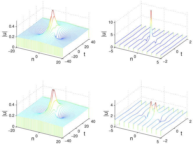
Figure 1: Stationary fundamental rogue waves (12) in the focusing Ablowitz-Ladik equation. Top row: on-site waves ($n_{0}=0$); bottom row: inter-site waves ($n_{0}=1/2$); left column: broad waves ($\rho=0.2$); right column: narrow waves ($\rho=0.8$).

Now we consider moving rogue waves (10) with $\theta\neq 0,\pi$. These rogue waves have not been reported before [18]. Two such solutions, with $\rho=0.8,n_{0}=0$ and $\theta=-1.2,-0.2$ are displayed in Fig. 2. In the left figure, we see a rogue wave rising from the constant background, traversing across the lattice, and then disappearing into the background again. In the right figure, the traversing motion of the rogue wave is less visible, because this rogue wave rises to its peak amplitude and retreats back to the constant background more quickly.

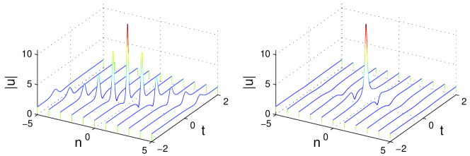
Figure 2: Moving fundamental rogue waves (10) in the focusing Ablowitz-Ladik equation with $\rho=0.8$ and $n_{0}=0$. Left: $\theta=-1.2$; right: $\theta=-0.2$.

When $\rho\to 0$, fundamental rogue waves (10) become very broad. In this case, the AL equation (1) reduces to the NLS equation, and rogue waves (10) approach the fundamental rogue waves of the NLS equation. In this limit, the parameter $\theta$ is the counterpart of the moving velocity of NLS rogue waves. The NLS equation admits Galilean invariance, thus any moving rogue wave can be derived from a stationary one through Galilean transformation. However, the AL equation is not Galilean invariant. Because of that, $\theta$ is a non-reducible parameter in rogue waves of the AL equation.

3.1.2 Defocusing case

Now we consider the defocusing case, where $|\rho|>1$, and solution (10) satisfies the defocusing AL equation (2). In this case, solution (10) still approaches the constant background as $t\to\pm\infty$, and rises to higher amplitude in the intermediate times, thus is also a rogue wave. The existence of rogue waves in the defocusing AL equation is surprising. Notice that the background amplitude $r$ of these rogue waves is always larger than 1 since $|\rho|>1$ [see Eq. (11)]. Indeed, we can show that in the defocusing AL equation, rogue waves with background amplitudes less than 1 cannot exist since such backgrounds are modulationally stable (see next subsection).

Rogue waves in the defocusing AL equation exhibit new features that have no counterparts in the focusing AL equation. Since $|\rho|>1$, the denominator in Eq. (10) may become zero, thus this rogue wave may blow up to infinity in finite time. To illustrate, let us take $\theta=0$. Then from the explicit expression (12), we see that this rogue wave will explode to infinity if

$$|n_{0}|<\frac{1}{2r},$$ (15)

where $r$ is the background amplitude in Eq. (11). When $n_{0}=1/2$, this rogue wave will be a regular rogue wave and never blow up since $r>1$. An example is shown in Fig. 3 (left) with $\rho=2$. This is an inter-site rogue wave, resembling that in Fig. 1 (lower right panel) of the focusing AL equation. However, if $n_{0}=0$, then the rogue wave (12) will always blow up. An example is shown in Fig. 3 (right) with $\rho=2$. We see that this rogue wave blows up to infinity at the lattice site $n=0$ and times $t=\pm 3\sqrt{3}/16$. At other $n_{0}$ values of $0<|n_{0}|<1/2$, this rogue wave will blow up for background values determined by the condition (15). The $n_{0}$-range for wave blowup shrinks as the background amplitude increases.

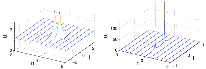
Figure 3: Fundamental rogue waves (10) in the defocusing Ablowitz-Ladik equation with $\theta=0$ and $\rho=2$. Left: $n_{0}=1/2$; right: $n_{0}=0$.

One may recall that exploding rogue waves have also been reported for the Davey-Stewartson (DS) II equation [17]. However, blowup in the DSII equation appears only for second- and higher-order rogue waves, but the blowup here occurs even for fundamental rogue waves (with $N=1$).

3.1.3 Connection with modulation instability

Why do rogue waves with background amplitudes higher than 1 exist in the defocusing AL equation? The reason is that such backgrounds are modulationally unstable. This modulation instability is analyzed below.

The defocusing AL equation (2) admits a constant-background solution

$$u_{n}(t)=r\hskip 0.85355pte^{-2i(1-r^{2})t},$$ (16)

where $r$ is the background amplitude. To study the modulation instability of this constant-background solution, we perturb this solution by normal modes

$$u_{n}(t)=e^{-2i(1-r^{2})t}\left(r+fe^{\lambda t+i\beta n}+\bar{g}e^{\bar{\lambda}t-i\beta n}\right),$$ (17)

where $\lambda$ and $\beta$ are the growth rate and wavenumber of the perturbation, and $f,g\ll 1$. Substituting this perturbed solution in Eq. (2) and neglecting terms of higher order in $f$ and $g$, we obtain the following equation for the growth rate $\lambda$,

$$\lambda^{2}=4(r^{2}-1)(1-\cos\beta)\left[(r^{2}+1)+(r^{2}-1)\cos\beta\right].$$ (18)

This formula shows that when the background amplitude $r>1$, $\lambda^{2}$ is positive for all wavenumbers $\beta$ with $\cos\beta\neq 1$, thus this constant background is modulationally unstable. As a consequence, rogue waves with background amplitudes higher than 1 can exist in the defocusing AL equation (2).

For lower background amplitudes $0<r<1$, however, the formula (18) shows that $\lambda^{2}$ is never positive for any wavenumber $\beta$, thus backgrounds lower than 1 are modulationally stable in the defocusing AL equation. Consequently rogue waves with such lower backgrounds cannot exist.

This modulation stability analysis can also be performed for the focusing AL equation (1). In this case, the constant-background solution is

$$u_{n}(t)=r\hskip 0.85355pte^{-2i(1+r^{2})t}.$$

Perturbing this solution by normal modes similar to (17) and following similar procedures, we can obtain the following equation for the growth rate $\lambda$,

$$\lambda^{2}=4(r^{2}+1)(1-\cos\beta)\left[(r^{2}-1)+(r^{2}+1)\cos\beta\right].$$

This formula shows that, for any background amplitude $r$, $\lambda^{2}$ is positive for wavenumbers $\beta$ with $\cos\beta>(1-r^{2})/(1+r^{2})$; thus all constant backgrounds in the focusing AL equation are modulationally unstable. This explains why rogue waves with arbitrary constant backgrounds exist in the focusing AL equation (1).

3.2 Second-order rogue waves

Now we consider second-order rogue waves in the AL equations. These second-order rogue waves can be obtained from formula (3) or (5) by taking

$$N=2,\;a_{1}=a_{2}=0,$$

and shifting $n$ to $n-n_{0}$, with $n_{0}$, $\theta$, $\rho$ and $a_{3}$ being free parameters. For simplicity, we take $\theta=0$ in our discussions below.

3.2.1 Focusing case

In this case, $|\rho|<1$. For $\rho=1/2$, four second-order rogue waves are displayed in Fig. 4 (the $n_{0}$ and $a_{3}$ parameters are specified in the captions). We see that these second-order rogue waves are all bounded (no blowup). In addition, they can exhibit either a single dominant hump (see panel (a)), or three humps (see panels (b-d)), depending on parameters. These behaviors are analogous to second-order rogue waves of the NLS equation [5, 6, 7, 8, 9, 10, 11, 12]. However, differences between AL and NLS rogue waves are also apparent. The main difference is that the three humps of the AL rogue waves generally have different heights, while those of the NLS rogue waves generally have the same height. The reason for this difference is that, in the AL rogue waves, some of these three humps are on-site and the others inter-site. On-site humps have higher heights than inter-site ones (see the previous subsection).

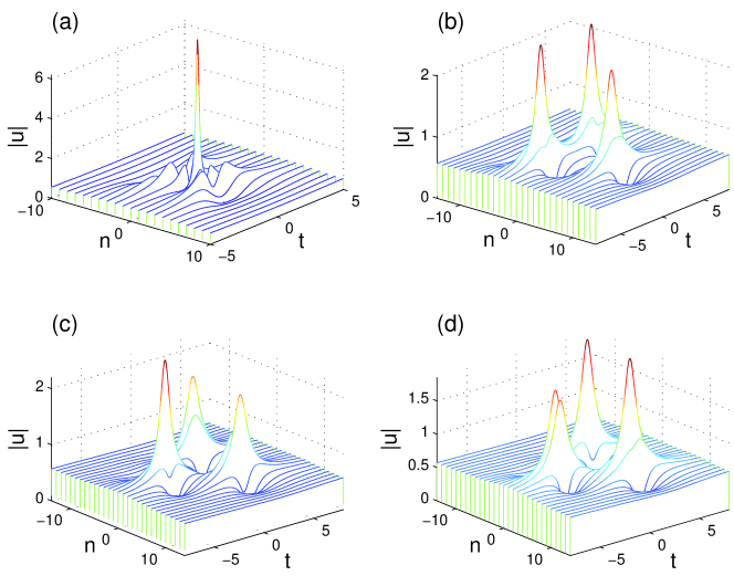
Figure 4: Second-order rogue waves in the focusing Ablowitz-Ladik equation for $\rho=1/2$ and $\theta=0$. (a) $n_{0}=-3/2,a_{3}=-1/54$; (b) $n_{0}=-3/2,a_{3}=5/3$; (c) $n_{0}=-3/2,a_{3}=5i/3$; (d) $n_{0}=0,a_{3}=5i/3$.

Second-order rogue waves in the focusing AL equation have been reported before [18]. Those rogue waves contain only two free real parameters (the counterparts of $\rho$ and $n_{0}$ in this article), thus they are a special class of second-order rogue waves. Due to the lack of the complex free parameter $a_{3}$, those second-order rogue waves in [18] cannot exhibit three-hump structures such as Fig. 4(b-d).

For each given $|\rho|<1$, we have also explored the rogue wave with the highest peak amplitude among all second-order rogue waves with free $n_{0}$ and $a_{3}$ values. We find that the highest possible peak amplitude is

$$|u|_{\mbox{\scriptsize max}}=r(5+20r^{2}+16r^{4}),$$ (19)

where $r=|\rho|/\sqrt{|1-\rho^{2}|}$ is the background amplitude [see Eq. (11)]. Interestingly, this highest-amplitude formula is identical to that reported in [18] even though the second-order rogue waves obtained in that work were special.

In this rogue wave with the highest peak amplitude (19), the corresponding $n_{0}$ and $a_{3}$ values are

$$n_{0,\hskip 1.42271pt\mbox{\scriptsize max}}=-\frac{1+\rho}{2\rho},\quad a_{3,\hskip 1.42271pt\mbox{\scriptsize max}}=\frac{1}{12}\frac{\rho-1}{(\rho+1)^{2}},$$ (20)

and this peak amplitude occurs at

$$n_{\mbox{\scriptsize max}}=0,\quad t_{\mbox{\scriptsize max}}=0.$$ (21)

For $\rho=1/2$, $n_{0,\hskip 1.13791pt\mbox{\scriptsize max}}=-3/2$, and $a_{3,\hskip 1.13791pt\mbox{\scriptsize max}}=-1/54$. The corresponding rogue wave is as displayed in Fig. 4(a). This rogue wave reaches peak amplitude $121/(9\sqrt{3})$, which is about 13 times higher than the background amplitude $1/\sqrt{3}$.

3.2.2 Defocusing case

Next we consider second-order rogue waves in the defocusing AL equation, where $|\rho|>1$. For $\rho=1.2$, four of these rogue waves are displayed in Fig. 5. We see that these second-order rogue waves can be bounded for certain parameter values (see panels (a,b)). However, for many other parameter values, they blow up in finite time (see panels (c,d)). This existence of both bounded and exploding second-order rogue waves is similar to that in fundamental rogue waves of the defocusing AL equation (see Fig. 3).

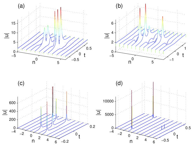
Figure 5: Second-order rogue waves in the defocusing Ablowitz-Ladik equation for $\rho=1.2$ and $\theta=0$. Top row: bounded rogue waves; bottom row: exploding rogue waves. The solution parameters are (a) $a_{3}=0,n_{0}=-0.38$; (b) $a_{3}=5/6,n_{0}=0$; (c) $a_{3}=0,n_{0}=0$; (d) $a_{3}=4/3,n_{0}=0$.

3.3 Higher-order rogue waves

Dynamics of third and higher order rogue waves in the AL equations can be studied in a similar way by using the general formula (3) or (5). For instance, we consider third-order rogue waves in the focusing AL equation by taking

$$N=3,\;\theta=0,\;\rho=1/2,\;a_{1}=a_{2}=a_{4}=n_{0}=0,$$

with $a_{3}$ and $a_{5}$ as free parameters. For four choices of ($a_{3},a_{5}$) values, the corresponding rogue waves are displayed in Fig. 6. It is seen that this rogue wave can exhibit a single high peak, or six lower peaks, depending on the ($a_{3},a_{5}$) values. Notice that the six peaks in Fig. 6 form triangular or circular patterns, analogous to the NLS equation [9, 10, 11]. However, the six peaks here have uneven amplitudes, unlike the NLS equation where the six peaks have almost identical amplitudes.

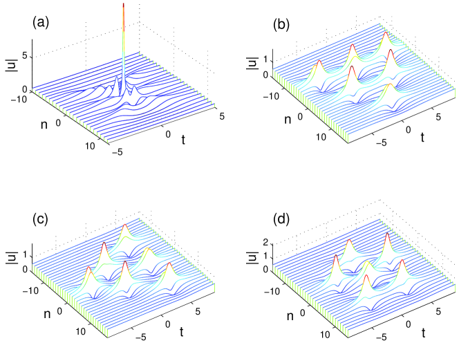
Figure 6: Third-order rogue waves in the focusing Ablowitz-Ladik equation for $\rho=1/2$, $\theta=0$ and $n_{0}=0$. (a) $a_{3}=a_{5}=0$; (b) $a_{3}=2,a_{5}=0$; (c) $a_{3}=2i,a_{5}=0$; (d) $a_{3}=0,a_{5}=2$.

4 Derivation of rogue-wave solutions

In this section, we derive general rogue-wave solutions and prove their boundary and regularity properties in Theorems 1-4.

We first establish a few lemmas. In Lemma 1 we introduce the so-called Grammian solutions to certain bilinear differential-difference equations, which are relevant to our study. By assuming that the matrix elements obey appropriate dispersion relations, we can show that the determinant (which we call $\tau$ function) satisfies these bilinear equations. If we choose suitable matrix elements, this $\tau$ function gives polynomial solutions, which is explained in Lemma 2. The next crucial step is to apply reduction to these polynomial solutions. This reduction is achieved in Lemma 3. Then by constraining parameters in the matrix elements, the $\tau$ function satisfies certain reality and conjugacy conditions, hence its bilinear equations reduce to the AL equations through a variable transformation. Rogue waves in the AL equations then are expressed through this $\tau$ function.

Lemma 1   Let $m_{ij}^{(n)}$, $\varphi_{i}^{(n)}$ and $\psi_{j}^{(n)}$ be functions of continuous independent variables $x$, $y$ and discrete ones $k$, $l$, satisfying the following differential and difference (dispersion) relations,

$$\begin{array}[]{l}\partial_{x}m_{ij}^{(n)}(k,l)=\varphi_{i}^{(n)}(k,l)\psi_{j}^{(n-1)}(k,l),\\[5.0pt] \partial_{y}m_{ij}^{(n)}(k,l)=\varphi_{i}^{(n-1)}(k,l)\psi_{j}^{(n)}(k,l),\\[5.0pt] m_{ij}^{(n+1)}(k,l)=(1-\rho^{2})m_{ij}^{(n)}(k,l)+\varphi_{i}^{(n)}(k,l)\psi_{j}^{(n)}(k,l),\\[5.0pt] m_{ij}^{(n)}(k+1,l)=(1-\rho^{2})m_{ij}^{(n)}(k,l)-\varphi_{i}^{(n-1)}(k+1,l)\psi_{j}^{(n)}(k,l),\\[5.0pt] m_{ij}^{(n)}(k,l+1)=(1-\rho^{2})m_{ij}^{(n)}(k,l)-\varphi_{i}^{(n)}(k,l)\psi_{j}^{(n-1)}(k,l+1),\\[5.0pt] \partial_{x}\varphi_{i}^{(n)}(k,l)=\varphi_{i}^{(n+1)}(k,l),\\[5.0pt] \partial_{y}\varphi_{i}^{(n)}(k,l)=-(1-\rho^{2})\varphi_{i}^{(n-1)}(k,l),\\[5.0pt] \varphi_{i}^{(n)}(k-1,l)=\varphi_{i}^{(n)}(k,l)-\varphi_{i}^{(n-1)}(k,l),\\[5.0pt] \varphi_{i}^{(n)}(k,l+1)=(1-\rho^{2})\varphi_{i}^{(n)}(k,l)-\varphi_{i}^{(n+1)}(k,l),\\[5.0pt] (\partial_{x}+1)\psi_{j}^{(n)}(k,l)=-\psi_{j}^{(n-1)}(k+1,l),\\[5.0pt] (\partial_{y}-1)\psi_{j}^{(n)}(k,l)=\psi_{j}^{(n+1)}(k,l-1),\\[5.0pt] \psi_{j}^{(n)}(k+1,l)=(1-\rho^{2})\psi_{j}^{(n)}(k,l)-\psi_{j}^{(n+1)}(k,l),\\[5.0pt] \psi_{j}^{(n)}(k,l-1)=\psi_{j}^{(n)}(k,l)-\psi_{j}^{(n-1)}(k,l).\end{array}$$ (22)

Then the determinant

$$\tau_{n}(k,l)=\det_{1\leq i,j\leq N}\left(m_{ij}^{(n)}(k,l)\right)$$

satisfies the bilinear equations

$$\begin{array}[]{l}(D_{x}+1)\tau_{n}(k-1,l)\cdot\tau_{n}(k,l)=\tau_{n+1}(k-1,l)\tau_{n-1}(k,l),\\ (D_{y}-1)\tau_{n}(k,l+1)\cdot\tau_{n}(k,l)=-\tau_{n-1}(k,l+1)\tau_{n+1}(k,l),\\ \tau_{n+1}(k-1,l)\tau_{n-1}(k,l+1)-(1-\rho^{2})\tau_{n}(k-1,l)\tau_{n}(k,l+1)\\ \hskip 147.95424pt=\rho^{2}\tau_{n}(k-1,l+1)\tau_{n}(k,l).\end{array}$$ (23)

Here $D$ is Hirota’s bilinear differential operator defined by

$$P(D_{x},D_{y})F(x,y)\cdot G(x,y)=P(\partial_{x}-\partial_{x^{\prime}},\partial_{y}-\partial_{y^{\prime}})F(x,y)G(x^{\prime},y^{\prime})|_{x^{\prime}=x,y^{\prime}=y},$$

and $P$ is a polynomial of $D_{x}$ and $D_{y}$.

Proof   By using the dispersion relations (22), we can show that the derivatives and shifts of the $\tau$ function are expressed by the bordered determinants as follows,

$$\partial_{x}\tau_{n}(k,l)=\left|\matrix{m_{ij}^{(n)}(k,l)&\varphi_{i}^{(n)}(k,l)\cr-\psi_{j}^{(n-1)}(k,l)&0}\right|,$$

$$\partial_{y}\tau_{n}(k,l)=\left|\matrix{m_{ij}^{(n)}(k,l)&\varphi_{i}^{(n-1)}(k,l)\cr-\psi_{j}^{(n)}(k,l)&0}\right|,$$

$$\tau_{n+1}(k,l)=(1-\rho^{2})^{N-1}\left|\matrix{m_{ij}^{(n)}(k,l)&\varphi_{i}^{(n)}(k,l)\cr-\psi_{j}^{(n)}(k,l)&1-\rho^{2}}\right|,$$

$$\tau_{n-1}(k,l)=\frac{1}{(1-\rho^{2})^{N}}\left|\matrix{m_{ij}^{(n)}(k,l)&\varphi_{i}^{(n-1)}(k,l)\cr\psi_{j}^{(n-1)}(k,l)&1}\right|,$$

$$\tau_{n}(k-1,l)=\frac{1}{(1-\rho^{2})^{N}}\left|\matrix{m_{ij}^{(n)}(k,l)&\varphi_{i}^{(n-1)}(k,l)\cr-\psi_{j}^{(n)}(k-1,l)&1}\right|,$$

$$\tau_{n}(k,l+1)=(1-\rho^{2})^{N-1}\left|\matrix{m_{ij}^{(n)}(k,l)&\varphi_{i}^{(n)}(k,l)\cr\psi_{j}^{(n-1)}(k,l+1)&1-\rho^{2}}\right|,$$

$$(\partial_{x}+1)\tau_{n}(k-1,l)=\frac{1}{(1-\rho^{2})^{N}}\left|\matrix{m_{ij}^{(n)}(k,l)&\varphi_{i}^{(n-1)}(k,l)&\varphi_{i}^{(n)}(k,l)\cr-\psi_{j}^{(n)}(k-1,l)&1&1\cr-\psi_{j}^{(n-1)}(k,l)&-1&0}\right|,$$

$$(\partial_{y}-1)\tau_{n}(k,l+1)=(1-\rho^{2})^{N-1}\left|\matrix{m_{ij}^{(n)}(k,l)&\varphi_{i}^{(n)}(k,l)&\varphi_{i}^{(n-1)}(k,l)\cr\psi_{j}^{(n-1)}(k,l+1)&1-\rho^{2}&1\cr-\psi_{j}^{(n)}(k,l)&1-\rho^{2}&0}\right|,$$

$$\tau_{n+1}(k-1,l)=\left|\matrix{m_{ij}^{(n)}(k,l)&\varphi_{i}^{(n)}(k,l)\cr-\psi_{j}^{(n)}(k-1,l)&1}\right|,$$

$$\tau_{n-1}(k,l+1)=\left|\matrix{m_{ij}^{(n)}(k,l)&\varphi_{i}^{(n-1)}(k,l)\cr\psi_{j}^{(n-1)}(k,l+1)&1}\right|,$$

$$\tau_{n}(k-1,l+1)=\frac{1}{\rho^{2}}\left|\matrix{m_{ij}^{(n)}(k,l)&\varphi_{i}^{(n)}(k,l)&\varphi_{i}^{(n-1)}(k,l)\cr-\psi_{j}^{(n)}(k-1,l)&1&1\cr\psi_{j}^{(n-1)}(k,l+1)&1-\rho^{2}&1}\right|.$$

By using the Jacobi formula of determinants, we obtain the identities,

$$[(\partial_{x}+1)\tau_{n}(k-1,l)]\tau_{n}(k,l)=\tau_{n}(k-1,l)\partial_{x}\tau_{n}(k,l)+\tau_{n+1}(k-1,l)\tau_{n-1}(k,l),$$

$$[(\partial_{y}-1)\tau_{n}(k,l+1)]\tau_{n}(k,l)=\tau_{n}(k,l+1)\partial_{y}\tau_{n}(k,l)-\tau_{n-1}(k,l+1)\tau_{n+1}(k,l),$$

$$\rho^{2}\tau_{n}(k-1,l+1)\tau_{n}(k,l)$$

$$=\tau_{n+1}(k-1,l)\tau_{n-1}(k,l+1)-(1-\rho^{2})\tau_{n}(k-1,l)\tau_{n}(k,l+1),$$

which completes the proof of bilinear equations (23).

The above lemma is quite powerful for constructing various types of solutions to bilinear equations (23), since the matrix elements can be any functions satisfying the dispersion relations (22). For example, a class of polynomial solutions can be obtained from it by the choice of matrix elements (see next lemma).

Lemma 2   We define matrix elements $m_{ij}^{(n)}$ by

$$m_{ij}^{(n)}(k,l)=A_{i}B_{j}m^{(n)}(k,l),$$

where

$$m^{(n)}(k,l)=\frac{1}{pq-1+\rho^{2}}(pq)^{n}\left(\frac{1-\rho^{2}-q}{1-1/p}\right)^{k}\left(\frac{1-\rho^{2}-p}{1-1/q}\right)^{l}e^{\xi+\eta},$$

$$\xi=px-\frac{1-\rho^{2}}{p}y,\quad\eta=-\frac{1-\rho^{2}}{q}x+qy,$$

$A_{i}$ and $B_{j}$ are differential operators with respect to $p$ and $q$ respectively, defined as

$$A_{i}=\sum_{\nu=0}^{i}\frac{a_{\nu}}{(i-\nu)!}[(p-1)\partial_{p}]^{i-\nu},$$ (24)

$$B_{j}=\sum_{\mu=0}^{j}\frac{b_{\mu}}{(j-\mu)!}[(q-1)\partial_{q}]^{j-\mu},$$ (25)

and $a_{\nu}$, $b_{\mu}$ are constants. Then for any sequences of indices $I_{1}$, $I_{2}$, $\cdots$, $I_{N}$ and $J_{1}$, $J_{2}$, $\cdots$, $J_{N}$, the determinant,

$$\tau_{n}(k,l)=\det_{1\leq i,j\leq N}\left(m_{I_{i},J_{j}}^{(n)}(k,l)\right)$$

satisfies the bilinear equations (23).

Proof    It is easy to see that the above $m^{(n)}(k,l)$ and

$$\varphi^{(n)}(k,l)=p^{n}(1-1/p)^{-k}(1-\rho^{2}-p)^{l}e^{\xi},$$

$$\psi^{(n)}(k,l)=q^{n}(1-\rho^{2}-q)^{k}(1-1/q)^{-l}e^{\eta}$$

satisfy the following differential and difference relations,

$$\partial_{x}m^{(n)}(k,l)=\varphi^{(n)}(k,l)\psi^{(n-1)}(k,l),$$

$$\partial_{y}m^{(n)}(k,l)=\varphi^{(n-1)}(k,l)\psi^{(n)}(k,l),$$

$$m^{(n+1)}(k,l)=(1-\rho^{2})m^{(n)}(k,l)+\varphi^{(n)}(k,l)\psi^{(n)}(k,l),$$

$$m^{(n)}(k+1,l)=(1-\rho^{2})m^{(n)}(k,l)-\varphi^{(n-1)}(k+1,l)\psi^{(n)}(k,l),$$

$$m^{(n)}(k,l+1)=(1-\rho^{2})m^{(n)}(k,l)-\varphi^{(n)}(k,l)\psi^{(n-1)}(k,l+1),$$

$$\partial_{x}\varphi^{(n)}(k,l)=\varphi^{(n+1)}(k,l),$$

$$\partial_{y}\varphi^{(n)}(k,l)=-(1-\rho^{2})\varphi^{(n-1)}(k,l),$$

$$\varphi^{(n)}(k-1,l)=\varphi^{(n)}(k,l)-\varphi^{(n-1)}(k,l),$$

$$\varphi^{(n)}(k,l+1)=(1-\rho^{2})\varphi^{(n)}(k,l)-\varphi^{(n+1)}(k,l),$$

$$(\partial_{x}+1)\psi^{(n)}(k,l)=-\psi^{(n-1)}(k+1,l),$$

$$(\partial_{y}-1)\psi^{(n)}(k,l)=\psi^{(n+1)}(k,l-1),$$

$$\psi^{(n)}(k+1,l)=(1-\rho^{2})\psi^{(n)}(k,l)-\psi^{(n+1)}(k,l),$$

$$\psi^{(n)}(k,l-1)=\psi^{(n)}(k,l)-\psi^{(n-1)}(k,l).$$

Thus

$$m_{ij}^{(n)}(k,l)=A_{i}B_{j}m^{(n)}(k,l),\hskip 5.69046pt\varphi_{i}^{(n)}(k,l)=A_{i}\varphi^{(n)}(k,l),\hskip 5.69046pt\psi_{j}^{(n)}(k,l)=B_{j}\psi^{(n)}(k,l)$$

satisfy the dispersion relations (22). Consequently the determinant $\tau_{n}(k,l)$ satisfies the bilinear equations (23). This completes the proof.

We note that the above $\tau_{n}(k,l)$ is not just a polynomial in $(x,y,k,l,n)$ but a polynomial times the exponential of a linear function, because the elements $m_{ij}^{(n)}(k,l)$ have the form of $(i+j)$-th degree polynomial of $(x,y,k,l,n)$ times $(pq)^{n}\left[(1-\rho^{2}-q)/(1-1/p)\right]^{k}\left[(1-\rho^{2}-p)/(1-1/q)\right]^{l}e^{\xi+\eta}$. The bilinear equations (23) are invariant when multiplying an exponential factor of a linear function in $(x,y,k,l,n)$ to $\tau_{n}(k,l)$. Thus through this gauge invariance, the solutions in Lemma 2 are equivalent to polynomial solutions. In this class of polynomials, there is a subclass of solutions which satisfy a certain reduction condition, which is described in the following lemma.

Lemma 3   The determinant

$$\tau_{n}(k,l)=\left.\det_{1\leq i,j\leq N}\left(m_{2i-1,2j-1}^{(n)}(k,l)\right)\right|_{p=q=1+\rho},$$ (26)

where $m_{ij}^{(n)}(k,l)$ is defined in Lemma 2, satisfies the reduction condition

$$\tau_{n}(k+1,l+1)=(1+\rho)^{4N}\tau_{n}(k,l).$$ (27)

Proof   We have

$$m^{(n)}(k+1,l+1)=\frac{1-\rho^{2}-q}{1-1/p}\ \frac{1-\rho^{2}-p}{1-1/q}\ m^{(n)}(k,l)$$

$$\qquad=\left(p+\rho^{2}+\frac{\rho^{2}}{p-1}\right)\left(q+\rho^{2}+\frac{\rho^{2}}{q-1}\right)m^{(n)}(k,l).$$

From the general Leibniz rule for high-order derivatives of a product function, we get the operator identity

$$[(p-1)\partial_{p}]^{\nu}\left(p-1+1+\rho^{2}+\frac{\rho^{2}}{p-1}\right)$$

$$=\sum_{\kappa=0}^{\nu}{\nu\choose\kappa}\left(p-1+\delta_{\kappa 0}(1+\rho^{2})+(-1)^{\kappa}\frac{\rho^{2}}{p-1}\right)[(p-1)\partial_{p}]^{\nu-\kappa}.$$

Using this identity, we get

$$A_{i}\left(p+\rho^{2}+\frac{\rho^{2}}{p-1}\right)$$

$$=\sum_{\nu=0}^{i}\sum_{\kappa=0}^{i-\nu}\frac{a_{\nu}}{\kappa!(i-\nu-\kappa)!}\left(p-1+\delta_{\kappa 0}(1+\rho^{2})+(-1)^{\kappa}\frac{\rho^{2}}{p-1}\right)[(p-1)\partial_{p}]^{i-\nu-\kappa}$$

$$=\sum_{\kappa=0}^{i}\frac{1}{\kappa!}\left(p-1+\delta_{\kappa 0}(1+\rho^{2})+(-1)^{\kappa}\frac{\rho^{2}}{p-1}\right)\sum_{\nu=0}^{i-\kappa}\frac{a_{\nu}}{(i-\nu-\kappa)!}[(p-1)\partial_{p}]^{i-\nu-\kappa}$$

$$=\sum_{\kappa=0}^{i}\frac{1}{\kappa!}\left(p-1+\delta_{\kappa 0}(1+\rho^{2})+(-1)^{\kappa}\frac{\rho^{2}}{p-1}\right)A_{i-\kappa},$$

and similarly

$$B_{j}\left(q+\rho^{2}+\frac{\rho^{2}}{q-1}\right)=\sum_{\lambda=0}^{j}\frac{1}{\lambda!}\left(q-1+\delta_{\lambda 0}(1+\rho^{2})+(-1)^{\lambda}\frac{\rho^{2}}{q-1}\right)B_{j-\lambda}.$$

Thus the matrix elements satisfy the relation

$$m_{ij}^{(n)}(k+1,l+1)=A_{i}B_{j}\left(p+\rho^{2}+\frac{\rho^{2}}{p-1}\right)\left(q+\rho^{2}+\frac{\rho^{2}}{q-1}\right)m^{(n)}(k,l)$$

$$=\sum_{\kappa=0}^{i}\frac{1}{\kappa!}\left(p-1+\delta_{\kappa 0}(1+\rho^{2})+(-1)^{\kappa}\frac{\rho^{2}}{p-1}\right)$$

$$\times\sum_{\lambda=0}^{j}\frac{1}{\lambda!}\left(q-1+\delta_{\lambda 0}(1+\rho^{2})+(-1)^{\lambda}\frac{\rho^{2}}{q-1}\right)m_{i-\kappa,j-\lambda}^{(n)}(k,l).$$

Substituting $p=1+\rho$ and $q=1+\rho$, we obtain the contiguity relation

$$\left.m_{ij}^{(n)}(k+1,l+1)\right|_{p=q=1+\rho}$$

$$=\sum_{\scriptstyle\kappa=0\atop\scriptstyle\kappa:{\rm even}}^{i}\frac{2\rho+\delta_{\kappa 0}(1+\rho^{2})}{\kappa!}\sum_{\scriptstyle\lambda=0\atop\scriptstyle\lambda:{\rm even}}^{j}\frac{2\rho+\delta_{\lambda 0}(1+\rho^{2})}{\lambda!}\left.m_{i-\kappa,j-\lambda}^{(n)}(k,l)\right|_{p=q=1+\rho},$$

from which the following matrix relation is derived:

$$\pmatrix{m_{11}^{(n)}(k+1,l+1)&m_{13}^{(n)}(k+1,l+1)&\cdots&m_{1,2N-1}^{(n)}(k+1,l+1)\cr m_{31}^{(n)}(k+1,l+1)&m_{33}^{(n)}(k+1,l+1)&\cdots&m_{3,2N-1}^{(n)}(k+1,l+1)\cr\vdots&\vdots&\ddots&\vdots\cr m_{2N-1,1}^{(n)}(k+1,l+1)&m_{2N-1,3}^{(n)}(k+1,l+1)&\cdots&m_{2N-1,2N-1}^{(n)}(k+1,l+1)}_{p=q=1+\rho}$$

$$=\pmatrix{(1+\rho)^{2}&0&\cdots&0\cr\displaystyle\frac{2\rho}{2!}&(1+\rho)^{2}&\cdots&0\cr\vdots&\vdots&\ddots&\vdots\cr\displaystyle\frac{2\rho}{(2N-2)!}&\displaystyle\frac{2\rho}{(2N-4)!}&\cdots&(1+\rho)^{2}}$$

$$\times\pmatrix{m_{11}^{(n)}(k,l)&m_{13}^{(n)}(k,l)&\cdots&m_{1,2N-1}^{(n)}(k,l)\cr m_{31}^{(n)}(k,l)&m_{33}^{(n)}(k,l)&\cdots&m_{3,2N-1}^{(n)}(k,l)\cr\vdots&\vdots&\ddots&\vdots\cr m_{2N-1,1}^{(n)}(k,l)&m_{2N-1,3}^{(n)}(k,l)&\cdots&m_{2N-1,2N-1}^{(n)}(k,l)}_{p=q=1+\rho}$$

$$\times\pmatrix{(1+\rho)^{2}&\displaystyle\frac{2\rho}{2!}&\cdots&\displaystyle\frac{2\rho}{(2N-2)!}\cr 0&(1+\rho)^{2}&\cdots&\displaystyle\frac{2\rho}{(2N-4)!}\cr\vdots&\vdots&\ddots&\vdots\cr 0&0&\cdots&(1+\rho)^{2}}.$$

By taking determinant of both sides, the reduction condition (27) is proved.

Proof of Theorem 1    Since the $\tau$ function (26) in Lemma 3 satisfies both the bilinear equations (23) and the reduction condition (27), it satisfies all the following bilinear equations,

$$(D_{x}+1)\tau_{n}(k,l)\cdot\tau_{n}(k+1,l)=\tau_{n+1}(k,l)\tau_{n-1}(k+1,l),$$

$$(D_{x}+1)\tau_{n}(k,l+1)\cdot\tau_{n}(k,l)=\tau_{n+1}(k,l+1)\tau_{n-1}(k,l),$$

$$(D_{y}-1)\tau_{n}(k,l+1)\cdot\tau_{n}(k,l)=-\tau_{n-1}(k,l+1)\tau_{n+1}(k,l),$$

$$(D_{y}-1)\tau_{n}(k,l)\cdot\tau_{n}(k+1,l)=-\tau_{n-1}(k,l)\tau_{n+1}(k+1,l),$$

$$\tau_{n+1}(k,l)\tau_{n-1}(k,l)-(1-\rho^{2})\tau_{n}(k,l)\tau_{n}(k,l)=\frac{\rho^{2}}{(1+\rho)^{4N}}\tau_{n}(k+1,l)\tau_{n}(k,l+1).$$

We now substitute $x=ict/(1-\rho^{2})$ and $y=-idt/(1-\rho^{2})$, where $c$ and $d$ are complex constants. Then the time derivative becomes $i(1-\rho^{2})\partial_{t}=-c\partial_{x}+d\partial_{y}$, and we obtain

$$[i(1-\rho^{2})D_{t}+c+d]\tau_{n}(k+1,l)\cdot\tau_{n}(k,l)$$

$$=c\tau_{n-1}(k+1,l)\tau_{n+1}(k,l)+d\tau_{n+1}(k+1,l)\tau_{n-1}(k,l),$$

$$[-i(1-\rho^{2})D_{t}+c+d]\tau_{n}(k,l+1)\cdot\tau_{n}(k,l)$$

$$=c\tau_{n+1}(k,l+1)\tau_{n-1}(k,l)+d\tau_{n-1}(k,l+1)\tau_{n+1}(k,l),$$

$$\tau_{n+1}(k,l)\tau_{n-1}(k,l)-(1-\rho^{2})\tau_{n}(k,l)\tau_{n}(k,l)=\frac{\rho^{2}}{(1+\rho)^{4N}}\tau_{n}(k+1,l)\tau_{n}(k,l+1).$$

The determinant solution (26) is now written as

$$\tau_{n}(k,l)=\left.\det_{1\leq i,j\leq N}\left(A_{2i-1}B_{2j-1}m^{(n)}(k,l)\right)\right|_{p=q=1+\rho},$$

where operators $A_{i}$, $B_{j}$ are defined in Eqs. (24)-(25), and

$$m^{(n)}(k,l)=\frac{1}{pq-1+\rho^{2}}(pq)^{n}\left(\frac{1-\rho^{2}-q}{1-1/p}\right)^{k}\left(\frac{1-\rho^{2}-p}{1-1/q}\right)^{l}e^{i\left(\frac{1}{pq}-\frac{1}{1-\rho^{2}}\right)\left(qd-pc\right)t}.$$

By taking $b_{\mu}=\bar{a}_{\mu}$ and $d=\bar{c}$, the conjugacy condition

$$\tau_{n}(l,k)=\overline{\tau_{n}(k,l)}$$

is then satisfied. We now define

$$f_{n}=\tau_{n}(0,0),\hskip 8.5359ptg_{n}=\tau_{n}(1,0)/(1+\rho)^{2N},$$ (28)

then $f_{n}$ is real, $\tau_{n}(0,1)/(1+\rho)^{2N}=\bar{g}_{n}$, and the above bilinear equations yield

$$[i(1-\rho^{2})D_{t}+c+\bar{c}]g_{n}\cdot f_{n}=cg_{n-1}f_{n+1}+\bar{c}g_{n+1}f_{n-1},$$

$$f_{n+1}f_{n-1}-(1-\rho^{2})f_{n}f_{n}=\rho^{2}g_{n}\bar{g}_{n}.$$

Finally we set $c=e^{-i\theta}$, where $\theta$ is a real constant. Then through the variable transformation,

$$u_{n}=\frac{\rho}{\sqrt{1-\rho^{2}}}\frac{g_{n}}{f_{n}}e^{i(\theta n-\omega t)},$$

where $\omega=(e^{i\theta}+e^{-i\theta})/(1-\rho^{2})=2\cos\theta/(1-\rho^{2})$, the above bilinear equations are transformed to

$$i\frac{d}{dt}u_{n}=(1+\sigma|u_{n}|^{2})(u_{n+1}+u_{n-1}),$$

where $\sigma=\mbox{sgn}(1-\rho^{2})$. Thus when $|\rho|<1$, the transformed equation is the focusing AL equation (1), while when $|\rho|>1$, the transformed equation is the defocusing AL equation (2). Then rogue wave solutions (3) for the focusing and defocusing AL equations are established [it is easy to see that functions $f_{n},g_{n}$ defined in Eq. (28) are identical to those given in Theorem 1]. The selection of parameters (4) can be proved in the same way as that for rogue waves of the NLS equation in [11] and is thus not repeated here. 

Proof of Theorem 2    By the reparametrization $p=1+\rho P$ and $q=1+\rho Q$, the matrix element $m_{ij}^{(n)}(k,l)=A_{i}B_{j}m^{(n)}(k,l)$ in Lemma 2 is given by

$$m^{(n)}(k,l)=\frac{(-1)^{k+l}\rho^{k+l-1}}{P+Q+\rho(1+PQ)}(1+\rho P)^{n+k}(1+\rho Q)^{n+l}\left(\frac{1+Q/\rho}{P}\right)^{k}\left(\frac{1+P/\rho}{Q}\right)^{l}e^{\xi+\eta},$$

$$\xi+\eta=\left(1+\rho P-\frac{1-\rho^{2}}{1+\rho Q}\right)x+\left(1+\rho Q-\frac{1-\rho^{2}}{1+\rho P}\right)y,$$

and

$$A_{i}=\sum_{\nu=0}^{i}\frac{a_{\nu}}{(i-\nu)!}(P\partial_{P})^{i-\nu},\quad B_{j}=\sum_{\mu=0}^{j}\frac{b_{\mu}}{(j-\mu)!}(Q\partial_{Q})^{j-\mu}.$$

Let us consider the following generator ${\cal G}$ of differential operators $(P\partial_{P})^{\alpha}(Q\partial_{Q})^{\beta}$,

$${\cal G}=\sum_{\alpha=0}^{\infty}\sum_{\beta=0}^{\infty}\frac{\kappa^{\alpha}}{\alpha!}\frac{\lambda^{\beta}}{\beta!}(P\partial_{P})^{\alpha}(Q\partial_{Q})^{\beta}=\exp(\kappa P\partial_{P}+\lambda Q\partial_{Q}).$$

Recalling the identity

$${\cal G}F(P,Q)=F(e^{k}P,e^{l}Q)$$

for any function $F$, applying ${\cal G}$ to the above $m^{(n)}$ and taking $P=Q=1$ (i.e. $p=q=1+\rho$), we have

$$\left.{\cal G}m^{(n)}(k,l)\right|_{P=Q=1}$$

$$=\frac{(-1)^{k+l}\rho^{k+l-1}}{e^{\kappa}+e^{\lambda}+\rho(1+e^{\kappa+\lambda})}(1+\rho e^{\kappa})^{n+k}(1+\rho e^{\lambda})^{n+l}\left(\frac{1+e^{\lambda}/\rho}{e^{\kappa}}\right)^{k}\left(\frac{1+e^{\kappa}/\rho}{e^{\lambda}}\right)^{l}e^{\tilde{\xi}+\tilde{\eta}}$$

$$=\frac{(-1)^{k+l}(1+\rho)^{2(n+k+l)-1}/2\rho}{\displaystyle 1-\frac{1-\rho}{1+\rho}\hskip 2.84544pt\frac{1-e^{\kappa}}{1+e^{\kappa}}\hskip 2.84544pt\frac{1-e^{\lambda}}{1+e^{\lambda}}}\exp\left[(n+k)\ln\frac{1+\rho e^{\kappa}}{1+\rho}+(n+l)\ln\frac{1+\rho e^{\lambda}}{1+\rho}\right.$$

$$\quad\left.+k\ln\frac{1+e^{\lambda}/\rho}{1+1/\rho}+l\ln\frac{1+e^{\kappa}/\rho}{1+1/\rho}-k\kappa-l\lambda-\ln\frac{1+e^{\kappa}}{2}-\ln\frac{1+e^{\lambda}}{2}+\tilde{\xi}+\tilde{\eta}\right],$$ (29)

where

$$\tilde{\xi}+\tilde{\eta}=\left(1+\rho e^{\kappa}-\frac{1-\rho^{2}}{1+\rho e^{\lambda}}\right)x+\left(1+\rho e^{\lambda}-\frac{1-\rho^{2}}{1+\rho e^{\kappa}}\right)y.$$

Differentiating the first expansion in (7) with respect to $\lambda$, we get

$$\frac{\rho e^{\lambda}}{1+\rho e^{\lambda}}=\frac{\rho}{1+\rho}+\sum_{\nu=1}^{\infty}(\nu+1)r_{\nu+1}(\rho)\lambda^{\nu},$$

thus $\tilde{\xi}+\tilde{\eta}$ can be written as

$$\tilde{\xi}+\tilde{\eta}=2\rho(x+y)+\left(\rho(e^{\kappa}-1)+(1-\rho^{2})\sum_{\nu=1}^{\infty}(\nu+1)r_{\nu+1}(\rho)\lambda^{\nu}\right)x$$

$$\hskip 36.98866pt+\left(\rho(e^{\lambda}-1)+(1-\rho^{2})\sum_{\nu=1}^{\infty}(\nu+1)r_{\nu+1}(\rho)\kappa^{\nu}\right)y.$$

Moreover since we have the formal expansion

$$\left[\displaystyle 1-\frac{1-\rho}{1+\rho}\hskip 2.84544pt\frac{1-e^{\kappa}}{1+e^{\kappa}}\hskip 2.84544pt\frac{1-e^{\lambda}}{1+e^{\lambda}}\right]^{-1}=\sum_{\mu=0}^{\infty}\left[\frac{1-\rho}{1+\rho}\hskip 2.84544pt\frac{\kappa\lambda}{4}\exp\left(\ln(\frac{2}{\kappa}\tanh\frac{\kappa}{2})+\ln(\frac{2}{\lambda}\tanh\frac{\lambda}{2})\right)\right]^{\mu},$$

Eq. (4) can be rewritten as

$$\frac{(-1)^{k+l}2\rho e^{-2\rho(x+y)}}{(1+\rho)^{2(n+k+l)-1}}\left.{\cal G}m^{(n)}(k,l)\right|_{P=Q=1}$$

$$=\sum_{\mu=0}^{\infty}\left(\frac{1-\rho}{1+\rho}\hskip 2.84544pt\frac{\kappa\lambda}{4}\right)^{\mu}\exp\left(\sum_{\nu=1}^{\infty}(x_{\nu}+\mu s_{\nu})\kappa^{\nu}+\sum_{\nu=1}^{\infty}(y_{\nu}+\mu s_{\nu})\lambda^{\nu}\right)$$

$$=\sum_{\mu=0}^{\infty}\left(\frac{1-\rho}{1+\rho}\hskip 2.84544pt\frac{\kappa\lambda}{4}\right)^{\mu}\sum_{\alpha=0}^{\infty}S_{\alpha}(\mbox{\boldmath$x$}+\mu\mbox{\boldmath$s$})\kappa^{\alpha}\sum_{\beta=0}^{\infty}S_{\beta}(\mbox{\boldmath$y$}+\mu\mbox{\boldmath$s$})\lambda^{\beta},$$

where $x_{\nu}$ and $y_{\nu}$ are as defined in Theorem 2. By taking the coefficient of $\kappa^{\alpha}\lambda^{\beta}$, we obtain

$$\frac{(-1)^{k+l}2\rho e^{-2\rho(x+y)}}{(1+\rho)^{2(n+k+l)-1}}\left.\frac{(P\partial_{P})^{\alpha}}{\alpha!}\frac{(Q\partial_{Q})^{\beta}}{\beta!}m^{(n)}(k,l)\right|_{P=Q=1}$$

$$=\sum_{\mu=0}^{\min(\alpha,\beta)}\frac{1}{4^{\mu}}\left(\frac{1-\rho}{1+\rho}\right)^{\mu}S_{\alpha-\mu}(\mbox{\boldmath$x$}+\mu\mbox{\boldmath$s$})S_{\beta-\mu}(\mbox{\boldmath$y$}+\mu\mbox{\boldmath$s$}).$$

Therefore the matrix element $m_{ij}^{(n)}(k,l)$ in Lemma 2 with $p=q=1+\rho$ is explicitly expressed in the polynomial form,

$$\left.\frac{(-1)^{k+l}2\rho e^{-2\rho(x+y)}}{(1+\rho)^{2(n+k+l)-1}}m_{ij}^{(n)}(k,l)\right|_{p=q=1+\rho}$$

$$=\sum_{\alpha=0}^{i}\sum_{\beta=0}^{j}\sum_{\mu=0}^{\min(i-\alpha,j-\beta)}\frac{a_{\alpha}b_{\beta}}{4^{\mu}}\left(\frac{1-\rho}{1+\rho}\right)^{\mu}S_{i-\alpha-\mu}(\mbox{\boldmath$x$}+\mu\mbox{\boldmath$s$})S_{j-\beta-\mu}(\mbox{\boldmath$y$}+\mu\mbox{\boldmath$s$}).$$

By taking $x=ite^{-i\theta}/(1-\rho^{2})$, $y=-ite^{i\theta}/(1-\rho^{2})$ and $b_{\beta}=\bar{a}_{\beta}$, the matrix element $m_{ij}^{(n)}(k,l)$ from the above equation is equal to $\widetilde{m}_{ij}^{(n)}(k,l)$ in Theorem 2, multiplied by a factor which is $(i,j)$-independent and is inversely proportional to $(-1)^{k}(1+\rho)^{2k}$. Recalling the definition of functions $f_{n},g_{n}$ in Eq. (28), $g_{n}/f_{n}$ in Theorem 1 is then equal to $(-1)^{N}\sigma_{n}(1,0)/\sigma_{n}(0,0)$, thus the algebraic expression of rogue waves in Eqs. (5)-(6) of Theorem 2 is proved.

The alternative expression (2) for $\sigma_{n}(k,l)$ in Theorem 2 can be derived directly from the original expression (6) through a similar determinant calculus in [11]. We rewrite the $N\times N$ determinant $\sigma_{n}(k,l)$ in (6) into a $3N\times 3N$ determinant form, then apply the Laplace expansion, which leads to the expression (2) (see [11] for details). Thus, Theorem 2 is proved.

Proof of Theorem 3    In the polynomial solution (2) in $n$ and $t$, the leading term comes from the one with $\nu_{1}=0$, $\nu_{2}=1$, $\ldots$, $\nu_{N}=N-1$, i.e.,

$$[(1-\rho)/(1+\rho)]^{N(N-1)/2}\det_{1\leq i,j\leq N}\left(\Phi_{2i-1,j-1}^{(n)}(k,l)\right)\det_{1\leq i,j\leq N}\left(\Psi_{2i-1,j-1}^{(n)}(k,l)\right).$$

Notice that the highest-degree terms in $\Phi_{i\nu}^{(n)}(k,l)$ and $\Psi_{j\nu}^{(n)}(k,l)$ are $a_{0}x_{1}^{i-\nu}/(i-\nu)!2^{\nu}$ and $\bar{a}_{0}y_{1}^{j-\nu}/(j-\nu)!2^{\nu}$ respectively. In addition, the leading term of $n$, $t$ in the product $x_{1}y_{1}$ is given by $|r_{1}(\rho)n+i(e^{-i\theta}\rho/(1-\rho^{2})-e^{i\theta}2r_{2}(\rho))t|^{2}=r_{1}(\rho)^{2}|n+i(e^{-i\theta}/(1-\rho)-e^{i\theta}/(1+\rho))t|^{2}$. Consequently the leading term of $n$, $t$ in the polynomial $\sigma_{n}(k,l)$ is proportional to

$$\left|n+i\left(\frac{e^{-i\theta}}{1-\rho}-\frac{e^{i\theta}}{1+\rho}\right)t\right|^{N(N+1)}=\left[\left(n+\frac{2t\sin\theta}{1-\rho^{2}}\right)^{2}+\left(\frac{2t\rho\cos\theta}{1-\rho^{2}}\right)^{2}\right]^{N(N+1)/2}.$$

If $\cos\theta\neq 0$, then this term is dominant as $n^{2}+t^{2}$ goes to infinity in any direction on the $(n,t)$-plane. The coefficient of this dominant term does not vanish and is independent of $k$ and $l$ by direct calculation. Thus if $\cos\theta\neq 0$, $\sigma_{n}(1,0)/\sigma_{n}(0,0)$ approaches 1 when the space-time point $(n,t)$ goes to infinity, for example, when $t$ goes to infinity (for each fixed $n$) or $n$ goes to infinity (for each fixed $t$). In addition, if $\cos\theta\neq 0$, then $\sigma_{n}(1,0)/\sigma_{n}(0,0)$ approaches 1 uniformly in $n$ as $|t|$ goes to infinity. Hence the boundary condition (9) in Theorem 3 is proved.

Proof of Theorem 4    From Theorem 2, we see that $\Psi_{i\nu}^{(n)}(k,l)$ is the complex conjugate of $\Phi_{i\nu}^{(n)}(l,k)$. Then from the expression of $\sigma_{n}(k,l)$ in Eq. (2), we have

$$\sigma_{n}(0,0)=\sum_{\nu_{1}=0}^{1}\sum_{\nu_{2}=\nu_{1}+1}^{3}\cdots\sum_{\nu_{N}=\nu_{N-1}+1}^{2N-1}\left(\frac{1-\rho}{1+\rho}\right)^{\nu_{1}+\nu_{2}+\cdots+\nu_{N}}\left|\det_{1\leq i,j\leq N}\left(\Phi_{2i-1,\nu_{j}}^{(n)}(0,0)\right)\right|^{2}.$$

Clearly $\sigma_{n}(0,0)\geq 0$ if $-1<\rho<1$. Furthermore the term for $\nu_{1}=1$, $\nu_{2}=3$, $\ldots$, $\nu_{N}=2N-1$ is not zero because $\Phi_{ii}^{(n)}(k,l)=a_{0}/2^{i}$ and $\Phi_{i\nu}^{(n)}(k,l)=0$ $(i<\nu)$. Therefore $\sigma_{n}(0,0)$ is strictly positive for $-1<\rho<1$. Consequently, rogue waves for the focusing AL equation in Theorems 1 and 2 are always non-singular, which completes the proof. 

Of course, this non-singularity of solutions does not hold for the defocusing AL equation (where $|\rho|>1$), as has been seen in Sec. 3.

5 Summary

In this paper, general $N$-th order rogue waves in the focusing and defocusing Ablowitz-Ladik equations were derived by the bilinear method. These solutions were given by determinants, and they contain $2N+1$ non-reducible free real parameters. In the focusing case, we showed that rogue waves are always bounded. In addition, they can reach much higher peak amplitudes than their continuous counterparts in the NLS equation. Furthermore, higher-order rogue waves can exhibit triangular and circular patterns with different individual peaks. In the defocusing case, we showed that rogue waves still appear, which is surprising. In this case, we found that rogue waves of any order can blow up to infinity in finite time, even though non-blowup rogue waves can also exist.

It is noted that solutions in the AL equations are closely related to those in the discrete Hirota equation [18]

$$i\frac{d}{dt}v_{n}=(1\pm|v_{n}|^{2})[(a+ib)v_{n+1}+(a-ib)v_{n-1}],$$ (30)

where $a$ and $b$ are any real constants. Since we have constructed rogue-wave solutions of the AL equations for arbitrary carrier wave frequency $\theta$, it is straightforward to derive rogue-wave solutions in the discrete Hirota equation as well. By writing $a+ib=Re^{i\Theta}$ with real constants $R$ and $\Theta$, we see that

$$v_{n}(t)=e^{-in\Theta}u_{n}(Rt)$$

is a solution of Eq. (30) when $u_{n}(t)$ is a solution of the AL equation (1) or (2). Thus, rogue-wave solutions for the discrete Hirota equation can be obtained directly from Theorem 1 or 2. For example, from Theorem 2 we get the following theorem. Here for simplifying the expression, the sign $(-1)^{N}$ in Theorem 2 is dropped and notations $\phi=\theta-\Theta$, $\Omega=R\omega$ are used.

Theorem 5   General $N$-th order rogue waves for the discrete Hirota equation (30) are given by

$$v_{n}(t)=\frac{\rho}{\sqrt{1-\rho^{2}}}\>\frac{\sigma_{n}(1,0)}{\sigma_{n}(0,0)}\hskip 4.26773pte^{i(\phi n-\Omega t)},$$

where $\rho$, $\phi$ are free real constants, $\Omega=[(a+ib)e^{i\phi}+(a-ib)e^{-i\phi}]/(1-\rho^{2})$, and $\sigma_{n}(k,l)$ is defined in Theorem 2 with $x$ and $y$ replaced by $it(a-ib)e^{-i\phi}/(1-\rho^{2})$ and $-it(a+ib)e^{i\phi}/(1-\rho^{2})$ respectively.

References

- [1] C. Kharif, E. Pelinovsky and A. Slunyaev, Rogue waves in the ocean (Springer, Berlin, 2009).
- [2] D. R. Solli, C. Ropers, P. Koonath and B. Jalali, “Optical rogue waves”, Nature 450, 1054–1057 (2007).
- [3] D. H. Peregrine, “Water waves, nonlinear Schrödinger equations and their solutions,” J. Australian Math. Soc. B, 25, 16-43 (1983).
- [4] N. Akhmediev, A. Ankiewicz, and J. M. Soto-Crespo, “Rogue Waves and Rational Solutions of the Nonlinear Schr dinger Equation,” Phys. Rev. E 80, 026601 (2009).
- [5] P. Dubard, P. Gaillard, C. Klein, V.B. Matveev, “On multi-rogue wave solutions of the NLS equation and positon solutions of the KdV equation”, Eur. Phys. J. Special Topics 185, 247-258 (2010).
- [6] P. Dubard, V.B. Matveev, “Multi-rogue waves solutions to the focusing NLS equation and the KP-I equation”, Nat. Hazards. Earth. Syst. Sci. 11, 667–672 (2011).
- [7] P. Gaillard, “Families of quasi-rational solutions of the NLS equation and multi-rogue waves”, J. Phys. A 44, 435204 (2011).
- [8] A. Ankiewicz, D.J. Kedziora and N. Akhmediev, “Rogue wave triplets”, Phys. Lett. A, 375, 2782–2785 (2011).
- [9] D.J. Kedziora, A. Ankiewicz, and N. Akhmediev, “Circular rogue wave clusters”, Phys. Rev. E 84, 056611 (2011).
- [10] B. Guo, L. Ling, and Q.P. Liu, “Nonlinear Schrödinger equation: Generalized Darboux transformation and rogue wave solutions”, Phys. Rev. E 85, 026607 (2012).
- [11] Y. Ohta and J. Yang, “General high-order rogue waves and their dynamics in the nonlinear Schrödinger equation”, Proc. Roy. Soc. A. 468, 1716-1740 (2012).
- [12] P. Dubard and V.B. Matveev, “Multi-rogue waves solutions: from the NLS to the KP-I equation”, Nonlinearity 26, R93-R125 (2013).
- [13] S. Xu, J. He and L. Wang, “The Darboux transformation of the derivative nonlinear Schr dinger equation”, J. Phys. A 44, 305203 (2011).
- [14] B. Guo, L. Ling and Q.P. Liu, “High-order solutions and generalized Darboux transformations of derivative nonlinear Schrödinger equations”, Stud. Appl. Math. 130, 317-344 (2013).
- [15] F. Baronio, M. Conforti, A. Degasperis and S. Lombardo, “Rogue Waves Emerging from the Resonant Interaction of Three Waves”, Phys. Rev. Lett. 111, 114101 (2013).
- [16] Y. Ohta and J. Yang, “Rogue waves in the Davey-Stewartson I equation,” Phys. Rev. E 86, 036604 (2012).
- [17] Y. Ohta and J. Yang, “Dynamics of rogue waves in the Davey-Stewartson II equation”, J. Phys. A 46, 105202 (2013).
- [18] A. Ankiewicz, N. Akhmediev, and J.M. Soto-Crespo, “Discrete rogue waves of the Ablowitz-Ladik and Hirota equations”, Phys. Rev. E 82, 026602 (2010).
- [19] A. Ankiewicz, J. M. Soto-Crespo, and N. Akhmediev, “Rogue waves and rational solutions of the Hirota equation”, Phys. Rev. E, 81, 046602 (2010).
- [20] Y.S. Tao and J.S. He, “Multisolitons, breathers, and rogue waves for the Hirota equation generated by the Darboux transformation”, Phys. Rev. E 85, 026601 (2012).
- [21] F. Baronio, A. Degasperis, M. Conforti1, and S. Wabnitz, “Solutions of the vector nonlinear Schrödinger equations: evidence for deterministic rogue waves”, Phys. Rev. Lett. 109, 044102 (2012).
- [22] N.V. Priya, M. Senthilvelan, and M. Lakshmanan, “Akhmediev breathers, Ma solitons, and general breathers from rogue waves: A case study in the Manakov system”, Phys. Rev. E 88, 022918 (2013).
- [23] L. Ling, B. Guo and L. Zhao, “High-order rogue waves in vector nonlinear Schrödinger equations”, arXiv:1311.2720 (2013).
- [24] J. He, S. Xu and K. Porsezian, “Rogue waves of the Fokas-Lenells equation”, J. Phys. Soc. Jpn. 81, 124007 (2012).
- [25] J. He, S. Xu, and K. Porsezian, “-order bright and dark rogue waves in a resonant erbium-doped fiber system”, Phys. Rev. E 86, 066603 (2012).
- [26] L. Zhao, C. Liu, and Z. Yang, “The rogue waves with quintic nonlinearity and nonlinear dispersion effects in nonlinear optical fibers”, arXiv:1312.3397 (2013).
- [27] B. Kibler, J. Fatome, C. Finot, G. Millot, F. Dias, G. Genty, N. Akhmediev, and J.M. Dudley, “The Peregrine soliton in nonlinear fibre optics”, Nature Physics, 6, 790–795 (2010).
- [28] A. Chabchoub, N. P. Hoffmann, and N. Akhmediev, “Rogue wave observation in a water wave tank”, Phys. Rev. Lett. 106, 204502 (2011).
- [29] A. Chabchoub, N. Hoffmann, M. Onorato, A. Slunyaev, A. Sergeeva, E. Pelinovsky, and N. Akhmediev, “Observation of a hierarchy of up to fifth-order rogue waves in a water tank”, Phys. Rev. E 86, 056601 (2012).
- [30] M. J. Ablowitz and J. F. Ladik, “A nonlinear difference scheme and inverse scattering”, Stud. Appl. Math. 55, 213-229 (1976).
- [31] M. J. Ablowitz and J. F. Ladik, “Nonlinear differential-difference equations and Fourier analysis”, J. Math. Phys. 17, 1011-1018 (1976).