Co-clustering of Fuzzy Lagged Data

Abstract

The paper focuses on mining patterns that are characterized by a fuzzy lagged relationship between the data objects forming them. Such a regulatory mechanism is quite common in real-life settings. It appears in a variety of fields: finance, gene expression, neuroscience, crowds and collective movements, are but a limited list of examples. Mining such patterns not only helps in understanding the relationship between objects in the domain, but assists in forecasting their future behavior. For most interesting variants of this problem, finding an optimal fuzzy lagged co-cluster is an NP-complete problem. We present a polynomial-time Monte-Carlo approximation algorithm for mining fuzzy lagged co-clusters. We prove that for any data matrix, the algorithm mines a fuzzy lagged co-cluster with fixed probability, which encompasses the optimal fuzzy lagged co-cluster by a maximum 2 ratio columns overhead and completely no rows overhead. Moreover, the algorithm handles noise, anti-correlations, missing values and overlapping patterns. The algorithm was extensively evaluated using both artificial and real-life datasets. The results not only corroborate the ability of the algorithm to efficiently mine relevant and accurate fuzzy lagged co-clusters, but also illustrate the importance of including fuzziness in the lagged-pattern model.

1 Introduction

A by-product of modern life is the ever growing trace of digital data; these might be pictures uploaded to the web, cellular trajectories collected by mobile providers, or the earth’s climate monitored by buoys, balloons and satellites. The feature common to such data is its temporal nature. Mining these data can facilitate uncovering the hidden regulatory mechanisms governing the data objects.

Early mining techniques used the key concept of clustering to look for patterns formed by a subset of the objects over all attributes, or vice versa [36, 12]. Following seminal work by Cheng and Church [17] in the area of gene expression using microarray technology, substantial focus has been placed in recent years on co-clustering [52, 40]. Co-clustering extends clustering by aiming to identify a subset of objects that exhibit similar behavior across a subset of attributes, or vice versa. Very few co-clustering studies have considered the problem of mining patterns that have a lagged correlation between a subset of the objects over a subset of the attributes [70, 85, 79]. For example, consider the problem of identifying a flock of pigeons from among a large collection of flight trajectories (that is, mining a coordinated movement of a subset of objects across a subset of time attributes) [56]. The flock’s spatial coordinated flight, where each member follows the leader with some lag (delay), is a lagged pattern comprising the flock members’ tempo-spatial locations (trajectories). The underlying assumption in these works is that the lagged correlation, if it exists, is fixed (i.e., with no noise whatsoever).

In real-life settings, however, lagged patterns are typically noisy. For example, consider the flock’s coordinated flight described above. Overall the flock maintains a general lagged flight formation (each member follows the leader with some lag). Yet, a closer look will reveal that each member deviates from that lag to some extent (due to wind changes, threats, physical strength, etc). The flock’s flight pattern can, however, be captured by a co-cluster comprising fuzzy lags.

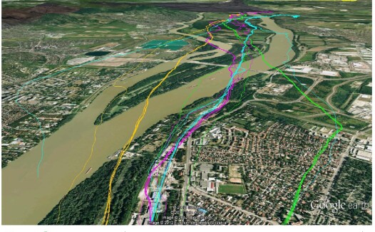
Figure 1: Snapshot of the flight of flocks of pigeon.

Fig. 1 presents such real-life flight trajectories, where each line represents a pigeon’s trajectory (pigeons belonging to the same flock are denoted by the same color). The presence of interleaving trajectories presents a serious challenge to mining algorithms (e.g., density-based algorithms [20]), as well as to humans (see Subsection 4.2). We denote a lagged co-cluster which includes a fuzzy correlation between a subset of objects over a subset of lagged attributes as a fuzzy lagged co-cluster. The problem, as later proved, is NP-complete for most interesting cases.

Similar fuzzy lagged behavior can be observed during the mining of a group of people that coordinate their movements within a crowd (e.g., a group of terrorists trying to move from point A to point B). The group would maintain a general lagged formation where each member follows the leader with some lag. However, due to obstacles, temporary loss of eye contact, and other difficulties, the group’s members would probably be compelled to deviate from that fixed lag. Additional motivation for studying fuzzy lagged co-clusters comes from the field of medicine within the context of disease relationships and causality. Given a dataset where an object is a disease, an attribute is an age, and an entry of the matrix is the number of occurrences of a disease in an age (the number of occurrences can be obtained from medical articles, hospital records, etc), the causality of diseases would be captured by a lagged co-cluster. However, the lag is expected to be of a fuzzy nature due to change in medical treatment, difference in disease development, inaccuracy of the dataset, etc. Mining such patterns can assist not only in the early detection of diseases, but also in providing better preventive treatment.

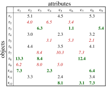
(a) Dataset

(b) Fuzzy lagged dataset

(c) Co-cluster

(d) Lagged co-cluster

(e) Fuzzy lagged co-cluster

Figure 2: Example of a fuzzy lagged dataset (based on [85]).

Fig. 2 presents an example of a fuzzy lagged dataset and various clusters within it. Fig. 2a depicts an example of a matrix dataset (for simplicity, certain cells have been left blank). Fig. 2b represents the same matrix after row permutation. Three clusters emerge, as follows. Fig. 2c (middle part of matrix 2b): a co-cluster with neither lag nor fuzziness. The value of a cluster entry, $A_{i,j}$, may deviates from being expressed as the sum of the column profile, $R_{i}$ (={3, 1, 2, 1} for row $i$={1, 4, 6, 11}, respectively), and the row profile, $C_{j}$ (={2, 1, 2} for column $j$={2, 5, 8}, respectively), by a maximum allowed error $\varepsilon\leq 0.5$. That is: $|(R_{i}+C_{j})-A_{i,j}|\leq\varepsilon=0.5$. Intuitively, the column profile indicates the regulation strength of the object, while the row profile indicates the regulatory intensity of the attribute. For example, the matrix entry of row $r_{4}$ and column $c_{8}$ is 3.2, which deviates from the expected value of: $R_{i}$+$C_{j}$=$R_{4}$+$C_{8}$=1+2=3, by an error of 0.2.

Fig. 2d (upper part of matrix 2b) exemplifies a lagged co-cluster, with no fuzziness. Here, the value of a cluster entry, $A_{i,j}$, may deviate from being expressed as $R_{i}+C_{j+T_{i}}$ by a maximum error of 0.5. That is: $|(R_{i}+C_{j+T_{i}})-A_{i,j}|\leq\varepsilon=0.5$. For example, the matrix entry of row $r_{7}$ and column $c_{3}$ is 8.4, which deviate from the expected value of: ($T_{7}$=–1) $R_{i}$+$C_{j+T_{i}}$=$R_{7}$+$C_{3+T_{7}}$=$R_{7}$+$C_{3-1}$=$R_{7}$+$C_{2}$=6+2=8, by an error of 0.4. Fig. 2e (lower part of matrix 2b) exemplifies a fuzzy lagged co-cluster. Here, the value of a cluster entry, $A_{i,j}$, not only may vertically deviate from being expressed as $R_{i}+C_{j+T_{i}}$ by a maximum error of 0.5, but also may horizontally deviate from $C_{j+T_{i}}$ by a maximum fuzziness, $F$, of two. That is: $|(R_{i}+C_{j+T_{i}+f_{i,j}})-A_{i,j}|\leq\varepsilon=0.5$, for some $\max_{i,j}\{f_{i,j}\}\leq 2$. For example, the matrix entry of row $r_{3}$ has a zero lag ($T_{3}$=0) and zero fuzziness over the columns $c_{3},c_{6}$ and $c_{9}$, i.e., $f_{3,j}=\{0,0,0\}$ (to ease readability, Fig. 2 does not present the fuzziness values). Relative to $r_{3}$, object $r_{8}$ has a lag of $T_{8}$=2 and fuzziness of $f_{8,j}=\{0,1,0\}$ (relative to $r_{3}$ columns); object $r_{10}$ has a lag of $T_{10}$=1 and fuzziness of $f_{10,j}=\{1,1,0\}$, and object $r_{12}$ has a lag of $T_{12}$=–1 and fuzziness of $f_{12,j}=\{-1,0,2\}$. For example, the matrix entry of row $r_{12}$ and column $c_{8}$ is 7.3, which deviate from the expected value of: ($T_{12}$=$-1$, $f_{12,c_{8}}$=2) $R_{i}$+$C_{j+T_{i}+f_{i,j}}$=$R_{12}$+$C_{8+T_{12}+f_{{12},8}}$=$R_{12}$+$C_{8-1+2}$=$R_{12}$+$C_{9}$=2+5=7, by an error of 0.3.

The main contribution of the paper is in introducing a polynomial time approximation algorithm for mining fuzzy lagged co-clusters, hereafter denoted as the FLC algorithm. To the best of our knowledge, this is the first attempt to develop such an algorithm. The input of the FLC algorithm is a real number matrix (where rows represent objects and columns represent attributes), a maximum error value and a maximum fuzziness degree. The algorithm uses a Monte-Carlo strategy to guarantee, with fixed probability, the mining of a fuzzy lagged co-cluster which encompasses the optimal fuzzy lagged co-cluster by a maximum 2 ratio columns overhead and completely no rows overhead. This guarantee holds for any monotonically increasing objective function defined over the cluster dimensions. Many of the inherent shortcomings common to non-fuzzy, non-lagged data [75, 12] are handled by the FLC algorithm, including noise (due to human or machine inaccuracies); missing values (e.g., equipment malfunction); anti-correlations (down-regulation, to adopt gene expression terminology) and overlapping patterns. The algorithm and its properties were extensively evaluated using both artificial and real-life datasets. The results not only corroborate the algorithm’s ability to efficiently mine relevant and accurate fuzzy lagged co-clusters, but also illustrate the importance of including fuzziness in the lagged-pattern model. With this inclusion, a significant improvement is achieved in both coverage and F₁ measures in comparison to using the regular (non-fuzzy) lagged co-clustering model. Moreover, the FLC algorithm presented classification capabilities which were superior to the ones presented by both the non-fuzzy lagged model and those of human subjects.

The remainder of the paper is organized as follows. Section 2 formally introduces the model and shows that most interesting variants of the problem are NP-complete. In Section 3 we present the algorithm followed by a run-time analysis, proof of the probabilistic guarantee to efficiently mine relevant fuzzy lagged co-clusters and extensions to the algorithm. Section 4 presents the experiments that were conducted and their results. In Section 5 we review related work. We conclude with a discussion and suggested directions for future research in Section 6.

2 Model

A lagged co-cluster of a real number matrix is a tuple $(I,T,J)$, representing a submatrix determined by a subset of the columns $J$ over a subset of the rows $I$ with their corresponding lags $T$ ($|T|$=$|I|$) [79] (see example in Fig. 2d). The fuzzy lagged co-clustering model augments the lagged co-cluster definition, enabling fuzziness in the lagged pattern.

Definition 1

A fuzzy lagged co-cluster of an $m\times n$ real number matrix $X$ is a tuple $(I,T,J,F)$, where $J$ is a subset of the columns, $I$ is a subset of the rows with their corresponding lags $T$, aligned to some fuzzy lagged mechanism by a maximal fuzziness degree of $F$ (see example in Fig. 2e). The fuzziness reflects the ability of a column to deviate from its lagged location, by a maximum of $F$ columns.

A fuzzy lagged regulatory mechanism holds if for all $j\in J$, each pair of rows $i_{1},i_{2}\in I$, their corresponding lags $T_{i_{1}},T_{i_{2}}$ and fuzziness $f_{i_{1},j},f_{i_{2},j}$, the proportion between the matrix entries is some constant, $C_{i_{1},i_{2}}$, dependent only on the rows $i_{1},i_{2}$ and independent of the columns $J$:

$$X_{i_{1},j+T_{i_{1}}+f_{i_{1},j}}/X_{i_{2},j+T_{i_{2}}+f_{i_{2},j}}=C_{i_{1},i_{2}}.$$

Let $G_{i}$ indicate the regulation strength of object $i$; $T_{i}$ indicate the influencing-lag of object $i$; $H_{j}$ indicate the regulatory intensity of attribute $j$; and $f_{i,j}$ indicate the fuzzy alignment of object $i$ to attribute $j$. Thus, the submatrix elements of a fuzzy lagged co-cluster should comply with the relation: $X_{i,j}\approx G_{i}H_{j+T_{i}+f_{i,j}}$ for all $i\in I$ and $j\in J$. We use the non-fuzzy lagged co-clustering relative error criteria [79, 70] to express the deviation of $X_{i,j}$ from the approximation of $G_{i}H_{j+T_{i}+f_{i,j}}$. Thus, our aim is to mine large submatrices which follow a fuzzy lagged regulatory mechanism, with a relative error below a pre-defined threshold:

$$\frac{1}{\eta}\leq\frac{G_{i}H_{j+T_{i}+f_{i,j}}}{X_{i,j}}\leq{\eta},\ \forall\ i\in I,\ j\in J.$$ (1)

To ease analysis, we move from a multiplicative model to an additive model. We do so by applying a logarithm transformation, setting $A_{i,j}$ = $\log(X_{i,j})$, $R_{i}$ = $\log(G_{i})$, $C_{j+T_{i}+f_{i,j}}$ = $\log(H_{j+T_{i}+f_{i,j}})$ and $\varepsilon$ = $\log(\eta)$. Therefore, our problem turns into finding $R_{i}$, $T_{i}$, $C_{j}$ and $f_{i,j}$, such that for all $i,j$:

$$-\varepsilon\leq R_{i}+C_{j+T_{i}+f_{i,j}}-A_{i,j}\leq\varepsilon.$$ (2)

The optimality of a submatrix depends on the objective function $\mu(I,J)$ being used. Examples of such common functions are: area: $\mu(I,J)=|I|\cdot|J|$; perimeter: $\mu(I,J)=|I|+|J|$; and $\mu(I,J)=|I|/{\psi}^{|J|},0<{\psi}<1$ [65, 53], which favors the inclusion of one column over the exclusion of a relatively large amount of rows. Such preferment of columns over rows appears mostly in biologically-oriented datasets where $m\gg n$ [40]. Nevertheless, for many fuzzy lagged datasets, assumptions relating to the number of rows vs. the number of columns is usually futile, i.e., a temporal dataset will usually contain thousands of time readings or, in an on-line version, an infinite stream of columns. Consequently, we allow the use of any monotonically growing objective function $\mu(I,J)$. Thus, our problem turns into mining an optimal size submatrix with a relative error below some given threshold.

Definition 2

The error of a submatrix $A$, defined by a subset $J$ of the columns, a subset $I$ of the rows and their corresponding lags $T$ is:

$$\varepsilon_{{}_{T,F}}(I,J)=\min_{R,C}\max_{i\in I,j\in J}|R_{i}+C_{j+T_{i}+f_{i,j}}-A_{i,j}|.$$ (3)

The error reflects the maximum deviation of a fuzzy lagged co-cluster’s entry, from being expressed as $R_{i}+C_{j+T_{i}+f_{i,j}}$.

At this point, we have all that is required to formally define a fuzzy lagged co-cluster. As mining small clusters, e.g., $[2\times 2]$, may not be of interest, we further extend the model to enable the user to specify the desired minimum dimensions: (1) minimum number of rows, expressed as a fraction of $m$, denoted $\beta$; and (2) minimum number of columns, expressed as a fraction of $n$, denoted $\gamma$.

Definition 3

Let $A$ be a matrix of size $m\times n$, $F\geq 0$ and $0<\beta,\gamma\leq 1$ constants independent of the matrix dimensions. A fuzzy lagged co-cluster of a matrix $A$ with an error $w\geq 0$ is a tuple $(I,T,J,F)$ with $J$ a subset of the columns, $I$ a subset of the rows with their corresponding lags $T$, which satisfies the following:

• Size: The number of rows is $2\leq\beta m\leq|I|$ and the number of columns is $2\leq\gamma n\leq|J|$.

• Fuzziness: $-F\leq f_{i,j}\leq F$, for all $i\in I$ and $j\in J$.

• Error: $\varepsilon_{{}_{T,F}}(I,J)\leq w$. i.e., for all $i\in I$ and $j\in J$ there exists $R_{i}$, $T_{i}$ and $C_{j}$, such that $|R_{i}+C_{j+T_{i}+f_{i,j}}-A_{i,j}|\leq w$. $R_{i},\ i\in I$ will be called a column profile, $T_{i},\ i\in I$ will be called a lagged column profile and $C_{j},\ j\in J$ will be called a row profile.

As a consequence, lagging row $i$ by $T_{i}$ and shifting it by $R_{i}$, will place each column $j\in J$, aligned with its fuzziness $f_{i,j}$, within a maximal error of $w$ of the row profile. The specific case of $f_{i,j}=0$ for all $i\in I$ and $j\in J$, is equivalent to the non-fuzzy lagged co-cluster definition given in the previous chapter.

2.1 Hardness Results

The complexity of the fuzzy lagged co-clustering problem depends on the nature of the cluster being mined, which is reflected by the objective function $\mu$ being used. Former literature has shown that many such non-fuzzy and non-lagged instances are NP-complete [49, 17, 70, 60].

Observation 1

Any hardness or inapproximability, resulting either from the non-fuzzy or the non-lagged problem, implies the same result for the fuzzy lagged problem.

Proof 2.1.

The fuzzy lagged co-clustering problem extends the lagged co-clustering problem ($f_{i,j}$=0, $\forall i\in I,j\in J$), which in turn extends the co-clustering problem ($T_{i}$=0, $\forall i\in I$). Thus, any valid instance of the non-fuzzy or the non-lagged problems can be seen as an instance of the fuzzy lagged problem. By negation, a polynomial time algorithm for the fuzzy lagged co-clustering problem would allow the lagged co-clustering problem or the co-clustering problem to be solved optimally in polynomial time – contradiction.

The following observation demonstrates a polynomial reduction between a fuzzy lagged instance and a non-fuzzy, non-lagged instance.

Observation 2

Let $A$ be a fuzzy lagged matrix of size $[m\times n]$ and for all ${i\in I}$, $|\{f_{i,j}:\forall j\in J,\ f_{i,j}\neq 0\}|\leq\log(mn)$. The matrix $A$ can be presented as a non-fuzzy, non-lagged matrix $A^{\prime}$, of size $[2mn{(2F+1)}^{\log(mn)}\times(3n+2F)]$.

Proof 2.2.

We duplicate each row $i\in A$, to represent all possible lags and fuzziness for that row. Each row $i$ $(1\leq i\leq m)$ can have $2n$ possible lags $(-n\leq$ lag $\leq n)$ and ${(2F+1)}^{\log(mn)}$ possible fuzziness (a maximum of $\log(mn)$ columns, each with a possible fuzziness assignment of: $-F\leq$ fuzziness $\leq F$), resulting in $(3n+2F)$ columns. Null entries resulting from such alignments, i.e., lag and fuzziness, are marked as missing values. The resulting non-fuzzy, non-lagged matrix $A^{\prime}$, is therefore of size $[m(2n){(2F+1)}^{\log(mn)}\times(3n+2F)]={\cal O}((mn)^{c})$ for some $c={\cal O}(\log(F))$. The result complies with a matrix of size $[2mn\times 3n]$ for the specific case of $F$=0 [70].

Corollary 2.3.

Let $A$ be a fuzzy lagged matrix. The problem of finding the largest square fuzzy lagged co-cluster $(I,T,$ $J,F)$ $(|I|$=$|J|)$ in $A$ is NP-complete.

Proof 2.4.

Following Observation 1, the fuzzy lagged co-clustering problem is NP-hard. Yet, verifying a submatrix of $A$ to be a fuzzy lagged co-cluster can be done in polynomial time by examining whether each entry holds the inequality of $-\varepsilon\leq R_{i}+C_{j+T_{i}+f_{i,j}}-A_{i,j}\leq\varepsilon$. Therefore the problem is NP-complete.

The following NP-complete approximations are worth mentioning [70]: approximating the size of the largest combinatorial square co-cluster with an approximation factor of $n^{1-\epsilon}$; approximating the size of the minimal sequential cluster-set for the co-clustering problem within a constant factor (Max-SNP-Hard); and, approximating the minimal set of combinatorial squares (co-cluster set) with an approximation factor of $n^{1-\epsilon}$.

3 The FLC Algorithm

We now present the FLC algorithm. This section also includes a proof for the algorithm’s guarantee to mine with fixed probability, in a polynomial number of iterations, a fuzzy lagged co-cluster that encompasses an optimal fuzzy lagged co-cluster. In addition, we supply a run-time analysis and several extensions.

3.1 The Algorithm

The input of the algorithm is: a matrix $A$ of real numbers; a maximum allowed error value $w$; a maximum allowed fuzziness degree $F$; a minimum fraction of the rows $\beta$; and, a minimum fraction of the columns $\gamma$. The algorithm itself uses a projected clustering approach. This common technique for mining co-clusters [49, 65] uses iterative random projection (i.e., a Monte-Carlo strategy) to obtain the cluster’s seed. It later grows the seed into a cluster. The output using this method is guaranteed, with fixed probability, to contain fuzzy lagged co-clusters that comply with the specified $\beta$, $\gamma$, $F$, and encompass the optimal fuzzy lagged co-cluster. Each mined cluster precisely obtains the rows and lags of the optimal cluster, with a maximum 2 ratio of its columns (i.e., a maximum addition of $J$ columns) and a maximum 2 ratio of its error.

Algorithm 1 presents the FLC algorithm. Generally, the algorithm can be divided into four stages, as follows. (1) Seeding (lines 1-1): a random selection of a row and a set of columns to serve as seeds. (2) Addition of rows (lines 1-1): we search for rows that reside within an error $w$ of the row and column profiles (see Def. 3). Unfortunately, these profiles are unknown. It may happen that the seed lies within the edge of the cluster. In such cases, rows situated on the other edge of the cluster would be within an error of $2w$. A naive exhaustive search is computationally not feasible, as there is an exponential number of combinations. To reduce this complexity, we use a sliding window technique. This technique enables a polynomial complexity. The window slides on the sorted set of events: $(A_{i,j+f}-A_{p,s})$, where $i\in m$, $j\in n$, $|f|\leq F$ and $s\in S$. In order to achieve an error of $2w$, we set the width of the sliding window to $4w$, which results in: $\varepsilon_{{}_{T,F}}(\{i,p\},J)=(\max_{j\in J}(A_{i,j+f}-A_{p,s})-\min_{j\in J}(A_{i,j+f}-A_{p,s}))/2=(4w)/2=2w$ (see Remark 3.16, below). (3) Addition of columns (lines 1-1): this is similar to the previous stage, but accumulating only columns that comply with the accumulated rows. (4) Polynomial repetition of the above steps (line 1) providing a guarantee to mine an encompassed optimal fuzzy lagged co-cluster.

1

Input: $A$, an $m\times n$ matrix of real numbers; $w$, the maximum acceptable error; $F$ the maximum degree of fuzziness; $\beta$, the minimum fraction of rows; and $\gamma$, the minimum fraction of columns.

2

Output: A collection of fuzzy lagged co-clusters $(I,T,J,F)$ whose error does not exceed $2w$.

3

Initialization: Setting $N$ and $|S|$ is thoroughly discussed in the following section.

4

5loop $N$ times

6      

7      // Initialization Phase

8      randomly choose a discriminating row $p:\ 1\leq p\leq m$

9       randomly choose a discriminating set of columns $S:\ S\subseteq n$

10       $I\leftarrow\{p\}$

11       $J\leftarrow S$

12      

13      // Row Addition Phase

14      foreach row $i:\ 1\leq i\leq m$ do

15             slide a $4w$ width window on $\{e_{s,j,f}\>|\>e_{s,j,f}=A_{i,j+f}-A_{p,s},\>\forall j\in n,\>\forall s\in S,\>-F\leq f\leq F\}$

16                   if $(\forall s\in S\ \exists t,\ \!t+\!s\!=\!j\!+\!f\;\wedge\;\exists e_{s,j,f}\!\in\!window)$ then

17                   // found a common lag $t$ for all $s\in\!S$

18                         add $(i,t)$ to $(I,T)$

19                        

20                  

21            

22      

23      // Column Addition Phase

24      randomly choose a discriminating column $s\in S$

25      

26      foreach column $j:\ 1\leq j\leq n$ do

27             slide a $4w$ width window on $\{e_{i}\>|\>e_{i}=A_{i,j+T_{i}+f}-A_{i,s+T_{i}},\>\forall i\in I,\>-F\leq f\leq F\}$

28                   if $(\forall i\!\in\!I\ \exists e_{i}\!\in\!window)$ then

29                         add $j$ to $J$

30                        

31                  

32            

33      

34      // Validation of Dimensions

35      if $|I|<\beta m$ or $|J|<\gamma n$ then

36             discard $(I,T,J,F)$

37            

38      

39

40return a collection of valid $(I,T,J,F)$

41

Algorithm 1 FLC algorithm

The FLC algorithm augments the (non-fuzzy) lagged co-clustering LC miner [70] to mine fuzzy lagged co-clusters. In addition, its improved design suggests a substantial improvement in run-time (in comparison to the LC miner) when mining non-fuzzy (i.e., $F$=0) clusters, from a run-time of ${\cal O}((mn)^{2-\log\gamma})$ [70, Section 6], to ${\cal O}((mn)^{1-\log\gamma}\>{\log}^{2}(mn))$ (see Subsection 3.2).

The nature of the FLC algorithm suggests that it is sensitive to the error being set. This key parameter needs to be carefully set in order to mine meaningful clusters. Setting it too high might result in many artifact clusters, while setting it too low might preclude valid clusters. To choose an appropriate error value, one can adopt any of the methods suggested for the non-fuzzy lagged co-clustering model [70].

Innately embedded within the algorithm are many desirable properties such as: (1) the ability to handle noise by allowing the fuzzy lagged co-cluster to deviate from the model (see Def. 3) by some pre-specified error. We accomplish this by using a window of width $4w$ as described above; (2) the ability to mine overlapping clusters by utilizing the Monte-Carlo strategy, which grows independent seeds into clusters on each repetitive run; (3) the ability to overcome missing values by calculating the coherence of a fuzzy lagged co-cluster on the non-missing values of the submatrix [83, 53]; and (4) anti-correlation (see Footnote 3). When both correlated and anti-correlated patterns may appear in the same fuzzy lagged co-cluster, one can exercise one of the following solutions: (i) duplicate each row of the input matrix to contain the anti-values of the row, i.e., for each row $i\in m$, add to the input matrix a new row containing the values of: $-A_{i,j},\ j\in n$; or (ii) the algorithm’s row addition phase (lines 1-1) should be modified into a two-pass sliding window. The first pass (similar to the current line 1) is over events of the type:
$\{e_{s,j,f}\>|\>e_{s,j,f}=A_{p,s}-A_{i,j+f},\>\forall j\in n,\>\forall s\in S,\>-F\leq f\leq F\},$
while the second pass is over events of the type:
$\{e_{s,j,f}\>|\>e_{s,j,f}=A_{p,s}+A_{i,j+f},\>\forall j\in n,\>\forall s\in S,\>-F\leq f\leq F\}.$
The intuition behind the second pass is that an anti-correlated value is basically the value of $(-A_{i,j})$. Therefore, the first sliding window pass, which includes events of $A_{p,s}-A_{i,j+f}$, should now be repeated over events of $A_{p,s}-(-A_{i,j+f})$, which equals to $A_{p,s}+A_{i,j+f}$.

3.2 Run-time

The row addition phase (lines 1-1) handles, for each of the $m$ rows, a sliding window of ${\cal O}(n\cdot|S|\cdot F)$ events. Therefore, its run-time is ${\cal O}(m\cdot{n|S|F}\cdot\log(n|S|F))$. In the same manner, the column addition phase (lines 1-1) handles, for each of the $n$ columns, a sliding window of ${\cal O}(mF)$ events. Therefore, its run-time is ${\cal O}(n\cdot{mF}\cdot\log(mF))$. Thus, the inner for-loops run-time is: ${\cal O}(mn\>\log(mn)\>\log(n)\>F)$.

The total number of iterations is bounded by Theorem 3.9 to $N={\cal O}(1/\beta\gamma^{|S|})$. Thus, for the constants $\beta$ and $\gamma$ independent of the matrix dimensions (see Def. 3), and the discriminating set $|S|={\cal O}(\log(mn))$ (see Theorem 3.6), the FLC’s total run-time is polynomial in the matrix size: ${\cal O}((mn)^{1-\log\gamma}\>{\log}^{2}(mn)\>F)$ which in many cases can be seen more permissibly as: ${\cal O}((mn)^{2-\log\gamma})$.

3.3 Sub-optimality of FLC Algorithm

Next, we analyze the ability of the FLC algorithm to mine coherent and relevant fuzzy lagged co-clusters. In particular we prove that the algorithm guarantees to mine, with fixed probability, in a polynomial number of iterations, a fuzzy lagged co-cluster that encompasses an optimal fuzzy lagged co-cluster. The mined cluster will acquire the rows of the optimal cluster and their lags with a maximum 2 ratio of its columns. Consequently, the mined cluster will have a maximum 2 ratio of the optimal cluster error. We demonstrate this guarantee with experiments on both artificial and real-life datasets in Section 4.

Since the FLC algorithm augments the non-fuzzy lagged co-clustering LC algorithm [70], its capabilities and theoretical analysis are deeply inspired by it. The structure of the proof consists of two major stages. The first stage is based on an important insight stating that a sufficient size for a discriminating set is logarithmic in the size of the set [65, 49]. Following this result, we show that by taking any small random subset of columns of size ${\cal O}(\log(mn))$, we can discriminate an optimal fuzzy lagged co-cluster with a probability of at least 0.5. The second stage utilizes the previous result to mine, in a polynomial number of iterations and with a probability of at least 0.5, clusters that encompass the optimal fuzzy lagged co-cluster.

The definition of a discriminating set for the fuzzy lagged model is given as follows.

Definition 3.5.

Let $(I,T,J,F)$ be a fuzzy lagged co-cluster with an error $w$ and $p\in I$. $S\subseteq J$ is a discriminating set for $(I,T,J,F)$ with respect to $p$ if it satisfies:

1. $\varepsilon_{{}_{T,F}}(\{i,p\},S)\leq w$ for all $(i,t)\in(I,T)$.

2. $\varepsilon_{{}_{T,F}}(\{i,p\},S)>w$ for all $(i,t)\notin(I,T)$.

The importance of using a discriminating set lies in its ability to discriminate, i.e., include fuzzy lagged rows which belong to the fuzzy lagged co-cluster and exclude those that do not. Therefore, as will be later shown, a discriminating set serving as a seed would grow in a deterministic way to a unique fuzzy lagged co-cluster, i.e., choosing a discriminating set more than once will yield the same fuzzy lagged co-cluster. Next, Theorem 3.6 states that for an optimal fuzzy lagged co-cluster $(I^{*},T^{*},J^{*},F)$, there is an abundance of small sub-sets of columns, each of which is a discriminating set with a probability of at least 0.5.

Theorem 3.6.

Let $(I^{*},T^{*},J^{*},F)$ be an optimal fuzzy lagged co-cluster of error $w$, with $\gamma\leq(|J^{*}|/n)<{\gamma^{\prime}}$, and let $p\in I^{*}$. Any randomly chosen columns subset $S$ of $J^{*}$, of size $|S|\geq\log(4mn)/\log(1/3{\gamma^{\prime}}(2F+1))$, is a discriminating set for $(I^{*},T^{*},J^{*},F)$, with respect to $p$, with a probability of at least $0.5$.

Let $(I^{*},T^{*},J^{*},F)$ be a fuzzy lagged co-cluster with a column profile $R^{*}_{i},\ i\in\!I^{*}$, a lagged column profile $T^{*}_{i},\ i\in\!I^{*}$ and a row profile $C^{*}_{j},\ j\in\!J^{*}$. We show that for any $S$ that satisfies the above, condition (1) of Def. 3.5 always holds and that the probability of condition (2) not to hold is less than $0.5$. This allows the probabilistic guarantee by the repeated execution.

Condition (1) is always satisfied, as $\{i,p\}\subseteq I^{*}$ and $S\subseteq J^{*}$. Therefore, $\varepsilon_{{}_{T,F}}(\{i,p\},S)\leq\varepsilon_{{}_{T^{*},F}}(I^{*},S)\leq\varepsilon_{{}_{T^{*},F}}(I^{*},J^{*})\leq w$, i.e., as being part of the optimal fuzzy lagged co-cluster, the error is not greater than $w$.

Moving to condition (2), we first extract an upper bound for the probability of $S$ to fail to be a discriminating set for $(I^{*},T^{*},J^{*},F)$ with respect to $p$, for a particular row, its corresponding lag and fuzziness. Based on all possible combinations of rows, lags and fuzziness, we calculate the lower bound for the probability of $S$ to discriminate, showing it to be greater than 0.5.

The subset $S$ fails to be a discriminating set for $(I^{*},T^{*},J^{*},F)$ with respect to $p$, only if there exists a fuzzy lagged row $i$ with it’s corresponding lag $t$, $(i,t)\notin(I^{*},T^{*})$, which fits the cluster, i.e., $\varepsilon_{{}_{T,F}}(\{i,p\},S)\leq w$. Next, we calculate a bound for the probability of this to hold for a particular row $i$, lag $t$ and fuzziness $f$. According to Def. 3, $\varepsilon_{{}_{T,F}}(\{i,p\},S)\leq w$ means that there are $R_{i}$, $T_{i}$, $f_{i,j}$, $R_{p}$, $T_{p}\>(=$0$)$, $f_{p,j}\>(=$$\{$0$\})$ and $C_{j},\ j\in S$, such that: $|A_{i,j}-R_{i}-C_{j+T_{i}+f_{i,j}}|\leq w$ and $|A_{p,j}-R_{p}-C_{j+T_{p}+f_{p,j}}|\leq w$ $\forall j\in S$. Shifting and aligning row $i\in I$ (in the first inequality) by $T_{i}$ and $f_{i,j}$ respectively, and subtracting the second inequality (of row $p$) we obtain, for all $j\in S$ and some $R\>(=R_{i}-R_{p})$:

$$|A_{i,j}-A_{p,j}-R|\leq 2w.$$ (4)

Next, we show that due to the optimality of the fuzzy lagged co-cluster, there are no more than $3|J^{*}|$ columns that satisfy the above equation for each row $i\in I$. If $|A_{i,j}-A_{p,j}-R|\leq 2w$ then: $-2w\leq A_{i,j}-A_{p,j}-R\leq 2w$. After adding $(A_{p,j}-C^{*}_{j}-R^{*}_{p})$ to both sides we obtain: $(A_{p,j}-C^{*}_{j}-R^{*}_{p})-2w\leq A_{i,j}-C^{*}_{j}-R^{*}_{p}-R\leq(A_{p,j}-C^{*}_{j}-R^{*}_{p})+2w$. Since $(I^{*},T^{*},J^{*},F)$ is an optimal fuzzy lagged co-cluster, then $|A_{p,j}-C^{*}_{j}-R^{*}_{p}|\leq w$ for all $j\in J^{*}$. Therefore, we obtain:

$$-3w\leq A_{i,j}-C^{*}_{j}-R^{*}_{p}-R\leq 3w.$$ (5)

We now present Lemma 3.7, which enables calculating a bound for the number of columns that satisfies Equation 5, i.e., columns that if considered to be part of the discriminating set will result in adding rows that do not belong to the optimal fuzzy lagged co-cluster.

Lemma 3.7.

Let $J\subseteq J^{*}$, and let $(i,t)\notin(I^{*},T^{*})$. If $|A_{i,j}-C^{*}_{j}-r|\leq w$ for some $r$ and all $j\in J$, then $J\subset J^{*}$.

Proof 3.8.

By negation, suppose that $(I,T,J,F)$ is a fuzzy lagged co-cluster that augments the optimal fuzzy lagged co-cluster $(I^{*},T^{*},J^{*},F)$ by using $J\supseteq J^{*}$, $I=I^{*}\cup\{i\}$ and $T=T^{*}\cup\{t\}$. The new cluster is a fuzzy lagged co-cluster of error $w$ satisfying $\mu(I,J)>\mu(I^{*},J^{*})$, hence contradicting the optimality of $(I^{*},T^{*},J^{*},F)$.

The result of Lemma 3.7 is that for a fuzzy lagged row $(i,t)\notin(I^{*},T^{*})$ there are at most $|J^{*}|$ columns that lie in an interval of length $2w$ (derived from $|A_{i,j}-C^{*}_{j}-r|\leq w$ of Lemma 3.7). Therefore, the interval $[-3w,3w]$ of Equation 5, which can be seen as the three intervals $[-3w,-w]$, $[-w,w]$ and $[w,3w]$, contains at most $3|J^{*}|$ columns that satisfy Equation 4. Choosing all columns of $S$ out of the above $3|J^{*}|$ columns would result in the inclusion of an undesirable fuzzy lagged row $(i,t)\notin(I^{*},T^{*})$. Therefore, choosing $|S|$ columns from the $3|J^{*}|$ columns out of the $n$ matrix columns has a probability which is bounded by: $(3|J^{*}|/n)^{|S|}\leq(3{\gamma^{\prime}})^{|S|}$.

The latter probability refers to a particular row $i$, lag $t$ and fuzziness $f$. The number of combinations for some row $i$ ($1\!\leq\!i\!\leq\!m$), some lag $t$ ($-n\!\leq\!t\!\leq\!n$) and some fuzziness $f$ ($-F\!\leq\!f\!\leq\!F$) is: $(m)(2n)(2F+1)^{|S|}$ (as each of the $|F|$ columns can be assignment with any fuzziness within the range $-F\!\leq\!f\!\leq\!F$). Therefore, the probability of not discriminating is bounded (after substituting $|S|\geq\log(4mn)/\log(1/3{\gamma^{\prime}}(2F+1))$) by: $2mn(2F+1)^{|S|}(3{\gamma^{\prime}})^{|S|}=2mn(3{\gamma^{\prime}}(2F+1))^{|S|}<0.5$.      This result of Theorem 3.6 is important since upon selecting $p\in I^{*}$ and $S\subseteq J^{*}$, we can deduce $I^{*}$ and $T^{*}$.

Moving to the second part of the proof, we show that when the FLC algorithm is run a polynomial number of iterations, it mines, with a probability of at least 0.5, a fuzzy lagged co-cluster encompassing the optimal fuzzy lagged co-cluster. We base this on Theorem 3.6, which shows the abundance of randomly selected discriminating sets of size ${\cal O}(\log(mn))$ with a discriminating probability of at least 0.5.

Theorem 3.9.

Let $S$ be a discriminating set for an optimal fuzzy lagged co-cluster $(I^{*},T^{*},J^{*},F)$ of error $w$. Provided $N\geq 2\ln 2/\beta\gamma^{|S|}$, the FLC algorithm will mine a fuzzy lagged co-cluster $(I,T,J,F)$ of error $2w$ such that: $I=I^{*}$, $T=T^{*}$, $J\supseteq J^{*}$ and $|J|\leq 2|J^{*}|$, with a probability of at least 0.5.

Since $|I^{*}|\geq\beta m$, the probability of choosing a row (see line 1) that satisfies $p\in I^{*}$ is at least $\beta$. As $|J^{*}|\geq\gamma n$, the probability of choosing a discriminating columns set (see line 1) which satisfies $S\subseteq J^{*}$ is at least $\gamma^{|S|}$. Following Theorem 3.6, any given $S\subseteq J^{*}$ is a discriminating set with a probability of at least $0.5$ with respect to $p$. Therefore, the probability that all $N$ iterations (see line 1) fail to find a discriminating row $p$ and a discriminating columns set $S$ is $(1-0.5\beta\gamma^{|S|})^{N}$. Substituting $N\geq 2\ln 2/\beta\gamma^{|S|}$ we obtain a maximum probability of $(1-0.5\beta\gamma^{|S|})^{2\ln 2/(\beta\gamma^{|S|})}$. Using the inequality $(1-1/x)^{x}<1/e$, for $x\geq 1$, with $x=\frac{2}{\beta\gamma^{|S|}}$ we get a probability that does not exceed $(1-\frac{\beta\gamma^{|S|}}{2})^{\frac{2}{\beta\gamma^{|S|}}\ln 2}<1/e^{ln2}=0.5$. It follows that the algorithm’s chances of mining a fuzzy lagged co-cluster upon a $p\in I^{*}$ and $S\subseteq J^{*}$ is at least $0.5$. When such a fuzzy lagged co-cluster is mined, we obtain from the discriminating property of $S$ (see Def. 3.5) that $I=I^{*}$ and $T=T^{*}$.

The following lemmas prove that the mined fuzzy lagged co-cluster contains $J^{*}$ and at most $|J^{*}|$ additional columns.

Lemma 3.10.

$|J|\leq 2|J^{*}|$, i.e., the size of the mined columns set $J$ is a maximum 2 factor of the size of the optimal cluster columns set $J^{*}$.

Proof 3.11.

A column $j$ is added to $J$ only if: $\max_{i}(A_{i,j+T_{i}+f}$-$A_{i,s+T_{i}})$-$\min_{i}(A_{i,j+T_{i}+f}$-$A_{i,s+T_{i}})$$\leq$4w (see lines 1-1), which is equal to $\varepsilon_{{}_{T,F}}(I,J)\leq 2w$ (see Remark 3.16, below, in the case of a matrix of two columns). Therefore, $\forall i\in I$ and $\forall j\in J$ there exists $R_{i}$, $T_{i}$, $C_{j}$ and $f_{i,j}$ such that: $-2w\leq R_{i}+C_{j+T_{i}+f_{i,j}}-A_{i,j}\leq 2w$. Since $I=I^{*}$, $T=T^{*}$ and initially $J=S\subseteq J^{*}$, we obtain from the optimality of $(I^{*},T^{*},J^{*},F)$, that for each of the intervals $[-2w,0]$ and $[0,2w]$, there are at most $|J^{*}|$ columns $j$ satisfying $|R^{*}_{i}+C^{*}_{j+T^{*}_{i}+f^{*}_{i,j}}-A_{i,j}|\leq w$. Thus, $J$ accumulates up to a maximum of $2|J^{*}|$ columns.

Lemma 3.12.

$J\supseteq J^{*}$, i.e., the mined columns set $J$ contains the optimal cluster columns set $J^{*}$.

Proof 3.13.

For each $j\in J^{*}$, we obtain from the optimality of ($I^{*},T^{*},J^{*},F)$ that $|A_{i,j}-R^{*}_{i}-C^{*}_{j+T^{*}_{i}+f^{*}_{i,j}}|\leq w$. Thus, $j$ will be added to $J$, namely $j\in J$.

As a consequence of Lemma 3.10, additional columns that are not in $J^{*}$ might be added. Yet the maximum number of added columns is $|J^{*}|$ (see Lemma 3.12) and the mined cluster will have a maximal error of $2w$.     

Remark 3.14.

The bound of $|S|\geq$ $\log(4mn)/$ $\log(1/3{\gamma^{\prime}}(2F+1))$ includes the parameter ${\gamma^{\prime}}$ whose value is not given as part of the problem input. In Subsection 4.1, we show experimentally that a random subset of size $0.6\log_{2}(4mn)-1$ will suffice, freeing the user from the burden of specifying the ${\gamma^{\prime}}$-related trade-off.

Remark 3.15.

Theorem 3.6 describes a discriminating set $S$ with a minimum discriminating probability of 0.5. In Subsection 4.1, we illustrate the relation between various magnitudes of $|S|$ and their discriminating probability.

Remark 3.16.

Theorem 3.6, Theorem 3.9 and Algorithm 1 all assume only the existence of the profiles $R^{*}_{i}$, $T^{*}_{i}$ and $C^{*}_{j}$. Although the actual values of the profile are not calculated in practice, an explicit calculation can be computed. In the case of a matrix $A$ of size [2$\times$k] (equivalent to [{i,p}$\times$S], see Def. 3.5), one can use the following polynomial technique [53, Subsection 4.1]. First, permute the columns of the matrix $A$ so that:

$$A_{1,1}-A_{2,1}\leq A_{1,2}-A_{2,2}\leq\cdots\leq A_{1,k}-A_{2,k}.$$

Next, set $w=[(A_{1,k}-A_{2,k})-(A_{1,1}-A_{2,1})]/2$, $h=[(A_{1,k}-A_{2,k})+(A_{1,1}-A_{2,1})]/2$ and let $\ell$ be such that: $A_{1,\ell}-A_{2,\ell}\leq h\leq A_{1,\ell+1}-A_{2,\ell+1}$. Then $R=<\!0,-h\!>$ and $C=<\!A_{1,1}+w,A_{1,2}+w,\ldots,A_{1,\ell}+w,A_{1,\ell+1}-w,\ldots,A_{1,k}-w\!>$. Therefore, we get $\varepsilon_{{}_{T,F}}(I,J)$=$[\max_{j\in J}(A_{1,j}-A_{2,j})-\min_{j\in J}(A_{1,j}-A_{2,j})]/2$, where $|I|$=2 and $|J|$=k.

For cases of a general matrix size, we refer the reader to Melkman et al. [53, Subsection 4.2], which is a discrete version of the Diliberto-Straus algorithm [18].

Remark 3.17.

Neither Theorem 3.6 nor Theorem 3.9 make any assumption whatsoever on the distribution of the data in the matrix nor on the distribution of the data in the fuzzy lagged co-cluster to be mined. The FLC algorithm is completely generic.

3.4 Extensions

Next, we present several extensions to the FLC algorithm and the resulting algorithmic modifications supporting these extensions.

3.4.1 Varying Fuzziness

A major characteristic of the FLC algorithm is the maximum allowed fuzziness $F$. This fuzziness is assumed to be common to all entries of the matrix. The algorithm can be extended to include a different maximum fuzziness for each row of the matrix, denoted ${F}_{i},\ i\in m$. To achieve this, the algorithm needs to be modified in the events which are later used by the sliding window (lines 1 and 1 of Algorithm 1). Essentially, the modification is in using the row’s maximum allowed fuzziness ${F}_{i}$ instead of the global fuzziness $F$. The modifications are as follows.

• Line 1, which accumulates rows, should be modified to:
  Slide a $4w$ width window on
  $\{e_{s,j,f}\>|\>e_{s,j,f}=A_{i,j+f}-A_{p,s},\>\forall j\in n,\>\forall s\in S,\>-{F}_{i}\leq f\leq{F}_{i}\}$.

• Line 1, which accumulates columns, should be modified to:
  Slide a $4w$ width window on
  $\{e_{i}\>|\>e_{i}=A_{i,j+T_{i}+f}-A_{i,s+T_{i}},\>\forall i\in I,\>-{F}_{i}\leq f\leq{F}_{i}\}$.

Similarly, the algorithm can also be extended to include a different maximum allowed fuzziness for each column of the matrix, denoted ${F}_{j},\ j\in n$.

3.4.2 Reduction in Size of the Discriminating Set

The discriminating set $S$, as shown by Theorem 3.6, is a small subset of size ${\cal O}(\log(mn))$. Nevertheless, the number of iterations $N$ required for achieving the probabilistic guarantee as shown by Theorem 3.9, is exponentially proportional to $|S|$. To improve the algorithm’s run-time, we propose to take a subset of the discriminating columns set $S$, denoted $S^{0}$, and assume it has zero fuzziness over all of the cluster’s rows, i.e., let $(I,T,J,F)$ be a fuzzy lagged co-cluster with a discriminating set of columns $S$, with the assumption that $f_{i,j}$=0, for all $i\in I,\ j\in S^{0}$. The assumption reduces the combinatorial number of rows that needs to be filtered by the discriminating set, and thus reduces the set size needed for the task (line 1 of Algorithm 1). However, this comes with the cost of limiting the nature of the clusters mined, i.e., fuzzy lagged co-clusters which do not have a minimum of $|S^{0}|$ columns of zero fuzziness would not be mined. To achieve that, we modify the FLC algorithm in the following way. Line 1, in addition to randomly choosing $S$, also randomly chooses $S^{0}\subseteq S$. Next, we modify line 1 to set the fuzziness $f$ such that if $s\in S^{0}$ then $f$=0, or otherwise $-F\!\leq\!f\!\leq\!F$. The results of an experiment to evaluate the effectiveness of this approach are reported in Subsection 4.1 (see Expt. II), revealing that even a moderated subset of $S$ for which a zero fuzziness is assumed, e.g., $|S^{0}|$=3, supplies a good balance between the gain in run-time and the constraint it implies on the model. Expt. IV suggests a technique which enables the use of an even lower discriminating set size.

3.4.3 Finding the Maximal Columns Set

As part of the process of column addition (lines 1-1 of Algorithm 1), each added column has its fuzziness setting. Nevertheless, when considering those settings in the context of a cluster, it may well happen that they do not co-exist. Take for example the following simple scenario: column $j_{1}$ has a fuzziness of $f_{i,j_{1}}$=$1$ and column $j_{2}$ has a fuzziness of $f_{i,j_{2}}$=$-1$, $\forall i\in I$. In the case of zero lag ($T_{i}$=0) and $j_{2}$=$j_{1}+1$, the cluster’s fuzziness setting would not be valid as although $j_{1}<j_{2}$, the actual matrix columns for $j_{1}$ and $j_{2}$ would be $j_{2}$ ($=j_{1}+1=j_{1}+f_{i,j_{1}}$) and $j_{1}$ ($=j_{2}-1=j_{2}+f_{i,j_{2}}$), respectively. In the case where $j_{1}<j_{2}$ are time points, we expect that their actual matrix entries will also maintain the same ordering relations (and not $j_{2}<j_{1}$).

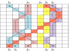
(a) A bridge matrix

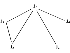
(b) Intersection graph

Figure 3: LABEL:sub@Algo:japaneses-bridges-example-matrix Example of a bridge matrix. Each color represents a different bridge. The lines related to each color represent the bridge graph. Take for example column $j_{2}$ and $j_{4}$. Assuming a zero lag (i.e., $T_{i}=0,\ \forall i\in I$), the column’s fuzziness is $\{0,1,0,0,1,0,0,0,0,-1,-1,0\}$ and $\{0,1,1,0,0,0,1,1,0,0,0,1\}$, respectively. LABEL:sub@Algo:japaneses-bridges-example-intersection The intersection graph of the bridge graph. The bridge of $j_{5}$ (red color) intersects all other bridges ($j_{1}$, $j_{2}$, $j_{3}$ and $j_{4}$). The bridges of $j_{1}$ (blue) and $j_{3}$ (wine) also intersect. All other bridges do not intersect (e.g., the bridges of $j_{2}$ (purple) and $j_{4}$ (yellow)). Therefore, the maximum non-intersecting set of bridges is either {$j_{1}$, $j_{2}$, $j_{4}$} or {$j_{3}$, $j_{2}$, $j_{4}$}.

One solution to this problem can be a post-processing step. We denote each of the columns’ fuzziness setting as a bridge, where the bridges are drawn on the discrete entries of the matrix $A$ (see example in Fig. 3a). We therefore wish to find the maximum non-intersecting set of bridges. To do so, consider the following problem: let $G$=$(V,E)$ be a bi-partite bridge graph with $|V|$=$n$ vertices on each side, and each edge $e$$\in$$E$ is a monotonic path between the upper and the lower side, i.e., a monotonous path of $\langle A_{i_{1},j_{1}},A_{i_{2},j_{2}},\ldots,A_{i_{k},j_{k}}\rangle$, where $i_{1}<i_{2}<\ldots<i_{k}$. The goal is to find the maximal set of non-intersecting edges in graph $G$. We do so by first showing in Lemma 3.18 that the intersection graph $\widehat{G}$ of the bridge graph $G$ (see example in Fig. 3b and 3a, respectively) is a perfect graph. Next, we conclude in Corollary 3.20 that the graph $G$ is also a perfect graph. As such, polynomial algorithms for finding a maximum clique can be applied, which results in finding the maximum set of non-intersecting columns’ bridges.

(a) Intersection Graph $\widehat{G}$

(b) Bridge Graph $G$

Figure 4: A graph is perfect if it cannot have a cycle of a minimum length of $5$ [66]. Fig. 4a presents a $5$-cycle intersection graph $\widehat{G}$. Fig. 4b illustrates the failure to draw the correlating $5$-cycle bridge graph $G$.

Lemma 3.18.

A bridge graph is a perfect graph.

Proof 3.19.

Let $\widehat{G}$ be the intersection graph of the bridge graph $G$. We show by negation that the intersection graph $\widehat{G}$ cannot have a cycle of a minimum length of $5$, and thus $\widehat{G}$ is a perfect graph [66]. Fig. 4 depicts the following steps.

1. By negation, let us assume that there is an intersection graph $\widehat{G}$ with a cycle of a minimum length $5$ (see Fig. 4a).

2. Let us denote the $5$ vertices of $\widehat{G}$ as $a$, $b$, $c$, $d$ and $e$.

3. Because $a$ and $c$ do not intersect, assume (w.l.o.g.) that $a$ is to the right of $c$ (see Fig. 4b).

4. Observe that because $c$ and $e$ do not intersect, $e$ cannot be to the left of $c$ as it should intersect $a$. Therefore $e$ is to the right of $c$.

5. $b$ intersects $c$ but does not intersect $e$. Therefore $e$ is to the right of $b$.

6. $d$ does not intersect $b$:

   (a) if $d$ is to the left of $b$ it cannot intersect $e$ – negation.

   (b) if $d$ is to the right of $b$ it must also be to the right of $a$ but then it cannot intersect $c$ – negation.

Corollary 3.20.

The algorithm’s column addition phase, which results in a maximum set of non-intersecting columns, has a polynomial run-time.

Proof 3.21.

Following Lemma 3.18, the intersection graph $\widehat{G}$ is a perfect graph. As the complement graph of a perfect graph is also a perfect graph [50], we can apply a maximum clique polynomial run-time procedure [29, 28] to the graph $G$ in order to acquire a maximum columns set.

4 Experiments

Next, we present an extensive evaluation of the FLC algorithm, using both artificial and real-life data.

4.1 Experiments with Artificial Data

In comparison to real-life data, the use of artificial data enables maximum control over the algorithm’s input and parameter settings, which in turn enables the verification and validation of the algorithm’s output. Specifically, the contributions of the experimentation used for the FLC algorithm with artificial data are threefold. First, it establishes default values for the various parameters. Second, it enables the verification of theoretical bounds. Finally, it demonstrates a feasible actual run-time.

Expt. I: Probability of Artifacts

An interesting question in the context of the fuzzy lagged model is how frequently artifacts are mined. An artifact is a submatrix that was formed not as a result of some hidden regulatory mechanism, but as a mere aggregation of noise. Such artifacts are undesirable as they add irrelevant output.

Given a matrix with randomly generated values (from a uniform distribution), the probability of mining an artifact fuzzy lagged co-cluster $(I,T,J,F)$ depends on several parameters: (1) the matrix dimensions, $[m\times n]$; (2) the fuzzy lagged co-cluster dimensions, $[|I|\times|J|]$; (3) the error $\varepsilon$, $0\%\leq\varepsilon\leq 100\%$; and (4) the fuzziness $F$. Intuitively, the larger the error $\varepsilon$, fuzziness $F$, and matrix size $m$ and $n$, and the smaller the requested cluster dimensions $I$ and $J$, the greater the chance of mining artifact clusters with an increasing probability of smaller clusters. To examine the correlation between these parameters, we present the following upper bound probability analysis.

Assume we know the column profile $p$. The probability of a column $j\in J$ of a fuzzy lagged row $i\in I$ to be within a surrounding of fuzziness $F$ and error $w$, encircling $p$ is: $1-(1-\min(2\varepsilon,1))^{2F+1}$. Hence, the probability of all columns $j\in J$ of a fuzzy lagged row $i\in I$ to be within a surrounding of fuzziness $F$ and error $w$, encircling $p$ is: $[1-(1-\min(2\varepsilon,1))^{2F+1}]^{|J|}$. Thus, the probability of all rows $I$ to form a fuzzy lagged co-cluster is: $[1-(1-\min(2\varepsilon,1))^{2F+1}]^{|I||J|}$. The probability of not having such a fuzzy lagged co-cluster is therefore: $1-[1-(1-\min(2\varepsilon,1))^{2F+1}]^{|I||J|}$. The representation of a fuzzy lagged matrix of size $[m\times n]$ as a non-lagged matrix, results in a matrix of size $[2mn\times 3n]$ (see Subsection 2.1). Thus, choosing a set size $|I|$ out of $(2mn)$ rows has $\binom{2mn}{|I|}$ combinations. Similarly, choosing a set size $|J|$ out of $(3n)$ columns has $\binom{3n}{|J|}$ combinations. Therefore, the probability that none of the possible sub-matrices of this size in the matrix forms a fuzzy lagged co-cluster is: $\{1-[1-(1-\min(2\varepsilon,1))^{2F+1}]^{|I||J|}\}^{\binom{2mn}{|I|}\binom{3n}{|J|}}$. Hence, an upper bound for the probability of at least one artifact fuzzy lagged co-cluster to exist is:

$$1-\{1-[1-(1-\min(2\varepsilon,1))^{2F+1}]^{|I||J|}\}^{\binom{2mn}{|I|}\binom{3n}{|J|}}.$$ (6)

As $\varepsilon$, $F$, $m$ and $n$ increase, the above probability will increase. As $I$ and $J$ increase the above probability will decrease.

To facilitate understanding of the formula, we present Fig. 5 and Fig. 6 (generated by Wolfram$|$Alpha [82]).

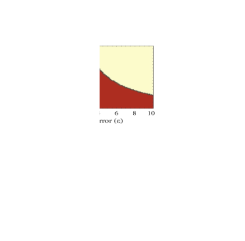
(a) $\beta$=1%, $\gamma$=1%.

(b) $\beta$=1%, $\gamma$=2%.

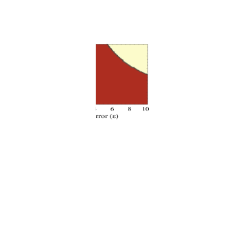
(c) $\beta$=1%, $\gamma$=4%.

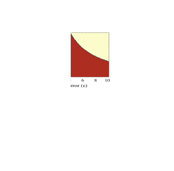
(d) $\beta$=2%, $\gamma$=1%.

(e) $\beta$=2%, $\gamma$=2%.

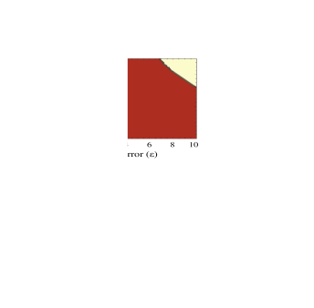
(f) $\beta$=2%, $\gamma$=4%.

(g) $\beta$=4%, $\gamma$=1%.

(h) $\beta$=4%, $\gamma$=2%.

(i) $\beta$=4%, $\gamma$=4%.

(j) $\beta$=7%, $\gamma$=7%.

Figure 5: Probability of an artifact fuzzy lagged co-cluster for various $\beta$ and $\gamma$, in a matrix of $[1000\times 1000]$. The red colored sections (bottom left area) represent a probability of 0.0. The light yellow colored sections (upper right area) represent a probability of 1.0. An interesting fact is the existence of a “phase transition”, where probabilities rapidly climb from 0.0 to 1.0, and its withdraw as $\beta$ and $\gamma$ increase. From the figures, we see that in this case a fuzzy lagged co-cluster of size greater than 0.5% of the matrix size has an insignificant probability to randomly appear.

(a) $\varepsilon$=1%, $F$=1.

(b) $\varepsilon$=1%, $F$=2.

(c) $\varepsilon$=1%, $F$=4.

(d) $\varepsilon$=5%, $F$=1.

(e) $\varepsilon$=5%, $F$=2.

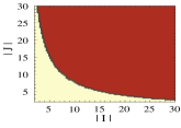
(f) $\varepsilon$=5%, $F$=4.

Figure 6: Probability of an artifact fuzzy lagged co-cluster for various $\varepsilon$ and $F$, in a matrix of $[1000\times 1000]$. The red colored sections (upper right area) represent a probability of 0.0. The light yellow colored sections (bottom left area) represent a probability of 1.0. The figures show the existence of the “phase transition”, where probabilities fall from 1.0 to 0.0, and its withdrawal as $\varepsilon$ and $F$ increase.

The main conclusion based on the figures is that fuzzy lagged co-clusters of small dimensions (i.e., clusters smaller than 0.5% of the matrix size) already have an insignificant probability of being caused by a random formation and presenting artifact patterns. Thus, fuzzy lagged co-clusters representing a regulatory mechanism, which are naturally large in dimensions, have an insignificant probability of being noise. Consequently, ordinary mining using practical dimensions has an insignificant probability of mining artifacts.

Expt. II: Discriminating Set Size

Theorem 3.6 provides us with the following bound for the discriminating set: $|S|\geq\log(4mn)/\log(1/3{\gamma^{\prime}}(2F+1))$, where ${\gamma^{\prime}}$ specifies the ratio between the number of columns in an optimal fuzzy lagged co-cluster and the number of matrix columns. The fact that the bound depends on ${\gamma^{\prime}}$ is undesirable, since this parameter is not part of the problem input and the user has no knowledge about it. To get a sense of the magnitude of feasible values for $|S|$, we conducted the following experiment. We first created random $[m\times n]$ matrices, with sizes ranging from $10^{2}$ to $10^{5}$ and values uniformly distributed in the range of $100$ to $1100$. We set the dimensions of the cluster size to $\beta,\gamma\in\{0.3,0.5,0.8\}$. Then, we generated a random fuzzy lagged co-cluster of error $\varepsilon$=1%, fuzziness $F$=1, size $[\beta m\times\gamma n]$ and put it at a random location in the matrix overriding the existing values. Then, a size - $k$ subset of the fuzzy lagged co-cluster columns was chosen at random $100$ times, to check whether it is a discriminating set according to Def. 3.5. This process was repeated for $k$=1,$\ldots$ until reaching a value for $k$ which the subset successfully discriminated in all of the $100$ trials. We repeated the above procedure for various sizes of $S^{0}$ in order to examine the effectiveness of $S^{0}$ in reducing the size of $S$ (see Subsection 3.4.2).

Fig. 7 presents the results of extensive experimentation relating to the trade-off between the size of the discriminating column set $|S|$ as a function of $\log_{2}(4mn)$ for various $|S^{0}|$.

Figure 7: The size of the discriminating column set $|S|$ as a function of $\log_{2}(4mn)$ for various $|S^{0}|$. The lower line of $|S^{0}|$$\rightarrow$$\infty$ represents the case of mining lagged clusters with no fuzziness ($F$=0).

The following important observations can be made from Fig. 7: (1) for each $|S^{0}|$ value used, we obtain the linear relationship derived from Theorem 3.6; (2) the decrease in size of the discriminating set $S$ is proportional to the size of $S^{0}$, i.e., the larger $|S^{0}|$ used, the lower $|S|$ needed. Setting $|S^{0}|$=3 seems to be the most effective in this case, as it offers a good balance between run-time reduction and the resultant limitation of the model (i.e., assuming $|S^{0}|$ non-fuzzy columns); and (3) we obtain an easy-to-use, ${\gamma^{\prime}}$ free, formula for setting $|S|$. For example, using $|S^{0}|$=3 we obtain: $|S|=0.6197\log_{2}(4mn)-1.0063\approx 0.6\log_{2}(4mn)-1$.

Expt. III: Discriminating Probability vs. Discriminating Set Size

The previous experiment considered a set of size $|S|$ to be discriminating if it successfully discriminated in all $N$ trials ($N$=100). In this experiment, we wish to explore the relationship between $|S|$ and its discriminating probability (i.e., in how many of the $N$ trials did the set actually discriminate). We do so by recording different sizes of $|S|$ and their ability to discriminate. The experiment was conducted using the same methodology as Expt. II, using $|S^{0}|$=3 as suggested.

Fig. 8 presents the discriminating probability as a function of the discriminating set size $|S|$.

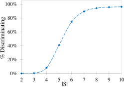
Figure 8: The discriminating probability as a function of the discriminating set size $|S|$. To facilitate reading, we only present the average results over $\beta,\gamma\in\{0.3,0.5,0.8\}$, as the results for the specific settings were of insignificant difference.

The main finding from Fig. 8 is that even for small sizes of $|S|$, a substantial discriminating probability is achieved (e.g., 89% for $|S|$=7). Since $|S|$ appears as an exponent in the estimated run-time, choosing a smaller $|S|$ will have a notable effect on the reduction of run-time, without having any major negative effects on the results.

Expt. IV: Discriminating Set Size vs. Number of Iterations Needed

Theorem 3.9 shows that the probability of the FLC algorithm to mine a fuzzy lagged co-cluster is at least 0.5. We refer to that probability as a “hit rate”. The hit rate depends on the discriminating probability $p$, of the discriminating set $S$, and the number of iterations $N$ being used: (hit rate) $=1-$ (miss rate) $=1-(1-p\beta\gamma^{|S|})^{N}$. Using Theorem 3.9, the number of iterations is $N$=$2\ln 2/\beta\gamma^{|S|}$, resulting in a hit rate of: $1-0.25^{p}$, i.e., (hit rate) $=1-(1-p\beta\gamma^{|S|})^{N}=1-(1-p\beta\gamma^{|S|})^{\frac{2\ln 2}{\beta\gamma^{|S|}}}=1-(1-p\beta\gamma^{|S|})^{\frac{p\cdot 2\ln 2}{p\cdot\beta\gamma^{|S|}}}\geq 1-\frac{1}{e^{2p\ln 2}}=1-\frac{1}{2^{2p}}=1-0.25^{p}$.

Expt. III implies that using a discriminating set smaller than the one recommended by Expt. II will not only exponentially decrease the run-time, but will also ensure a reasonable discriminating probability. However, a decrease in the discriminating set size results in a decrease in the hit rate. Therefore, in order to improve the hit rate, an increase in the number of iterations is required. In practice, by reducing the discriminating set size, it is possible to reduce the run-time by more than the increase needed to ensure the desired hit-rate.

We next present an analysis aimed at finding the best setting to achieve a minimum run-time. As a base line, we use Expt. II discriminating sets, with a discriminating probability of $\approx$100% and a size of 8.5 for matrices of size $[100\times 100]$. Such sets will yield a hit rate of $\approx$75%.

Based on the average curve, shown in Fig. 8, the discriminating probabilities of $|S|$={4, 5, 6, 7, 8, 9} are $P_{|S|}$={8.2%, 40.8%, 74.3%, 89.4%, 94.1%, 95.6%}, respectively. In order to reach a hit rate of 75%, we need to compensate for the loss in the above discriminating probability by increasing the number of iterations. Note that when the number of iterations $N$ is multiplied by $C$=$1/p$, the resulting hit rate becomes: $1-(1-p\beta\gamma^{|S|})^{(\frac{1}{p}\cdot N)}$ = $1-(1-p\beta\gamma^{|S|})^{\frac{2\ln 2}{p\beta\gamma^{|S|}}}$ $\geq$ $1-\frac{1}{e^{2\ln 2}}$ = $1-\frac{1}{2^{2}}$ = $0.75$. Therefore, by factoring the number of iterations ${N}(|S|)$=$2\ln{2}/(\beta\gamma^{|S|})$ by the inverse of the discriminating probability, we obtain for $|S|$={4, 5, 6, 7, 8, 9}, a ${C}_{|S|}$={1/8.2%, 1/40.8%, 1/74.3%, 1/89.4%, 1/94.1%, 1/95.6%}={12.24, 2.45, 1.35, 1.12, 1.06, 1.05}, respectively. Fig. 9 depicts the ratio between ${C}(|S|)$$\times$${N}(|S|)$ and the base line ${N}(8.5)$ for various $|S|\in[4-9]$. The ratio is independent of $\beta$ and equal to ${C}(|S|)\times{\gamma}^{(8.5-|S|)}$. The lower the ratio, the better the performance as less iterations are required.

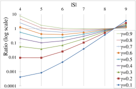
Figure 9: The ratio of iterations required for various $|S|$ to reach a 75% hit rate base line. The lower the ratio, the better the performance (i.e., less iterations required).

The main finding of the experiment is the ability to use discriminating sets with lower discriminating probability, compensated by a larger number of iterations to achieve the same hit rate levels while having lower run-time. An example from Fig. 9 is the preferable use of $|S|$=5 for $\gamma\leq$ 0.5 and $|S|$=6 for $\gamma\geq$ 0.6 over setting $|S|$=8.

Expt. V: Run-time, Number of Iterations and Hit Rate

Theorem 3.9 states that for any given discriminating set with a discriminating probability of 0.5 (see Theorem 3.6) and for $N\geq 2\ln{2}/(\beta\gamma^{|S|})$ trials, we are guaranteed to find a factor 2 optimal fuzzy lagged co-cluster with a probability of at least $0.5$. We report on the actual performance of the algorithm in mining an optimal fuzzy lagged co-cluster in terms of those three parameters.

The experiment was conducted by creating a random matrix of size $[100\times 100]$ and randomly placing random fuzzy lagged co-clusters of varying sizes (i.e., $\beta,\ \gamma\in\{0.3,0.5,0.8\}$) overriding the original values. To obtain sets with a discriminating probability of 0.5, we set $|S|$=5 with a discriminating probability of 40.8% (see Expt. III). While repeating the execution of the algorithm 10,000 times for each cluster size $\beta,\ \gamma\in$ {0.3, 0.5, 0.8}, we counted:

(1) hit rate: how many times out of the 10,000 repetitions the algorithm managed to mine the planted cluster; (2) iterations: how many iterations it took in practice to mine the optimal cluster; and (3) run-time: how long (in minutes) it took to mine the optimal cluster. The experiment was conducted using the platform: Intel core i7 @ 2.00GHz CPU with 6GB RAM, Windows 7 64 bit. The algorithm was programmed in Java 7.0. The results obtained are as follows.

• Hit Rate: An actual average hit rate of 44.0%, higher than the expected hit rate of 43.2% for a discriminating set with a discriminating probability of 40.8%.

• Number of Iterations:

  

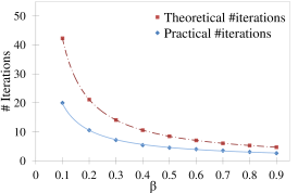
  Figure 10: Number of iterations required to mine a fuzzy lagged co-cluster vs. the theoretical bound. We present here only the results of $\gamma$=0.8, as the results for the other $\gamma$ values were insignificantly different. Since both $\gamma$ and $|S|$ were held fixed at $0.8$ and $5$, respectively, both theoretical and practical situations present a behavior of $N$=${\cal O}(1/\beta)$.

  Fig. 10 presents the actual number of iterations needed to mine the optimal fuzzy lagged co-cluster in relation to the theoretical boundary. On average, the actual number of iterations needed is 49% of the specified theoretical bound.

• Run-time: The run-time boundary, as specified by Subsection 3.2 is: $t$ = ${\cal O}((mn)^{2}/\gamma^{|S|})$. Fitting the actual run-time to an equation of type: $t$=$c/(\beta^{x}\gamma^{y})$ ($t$ in ms), where $c=(mn)^{2}$, we obtain: $x=0.83$, $y=4.49$ and $c=107.2$. As expected, the power of $\beta$ is close to 1 and the power of $\gamma$ is close to 5 (we set $|S|$=5). These results are better than the theoretical bound due to $\beta,\gamma\leq 1.0$.

To summarize, on our test set the FLC algorithm manages to mine fuzzy lagged co-clusters with a hit rate higher than the expected hit rate, less than 50% of the needed theoretical number of iterations, and does so within a feasible run-time.

Expt. VI: The Effect of Error and Fuzziness

The main objective of the previous experiments was to demonstrate properties of the fuzzy lagged co-clustering model while focusing on the correctness of the theoretical bounds of Algorithm 1. In this experiment, we wish to examine the extent of changes in the mining results as a function of the error and fuzziness used. To do so, we planted random fuzzy lagged co-clusters of specific error and fuzziness and set the miner’s parameters of error and fuzziness to various values.

To measure how well the miner performed in each setting, we used the complement of the RNIA score [59], defined as follows. Let $C_{1}$ and $C_{2}$ be fuzzy lagged co-clusters. $RNIA(C_{1},C_{2})=(|U|-|I|)/|U|$, where $U$ and $I$ are the matrix elements in the union and intersection of $C_{1}$ and $C_{2}$, respectively. Hence, $1\!-\!RNIA$$(C_{1},C_{2})$=$|I|/|U|$, achieves a score of $1$ when $C_{1}$ and $C_{2}$ are equal, and a score of $0$ when completely disjoint.

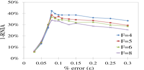
(a) Planted cluster: $\varepsilon$=0.1%, $F$=4.

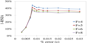
(b) Planted cluster: $\varepsilon$=0.01%, $F$=4.

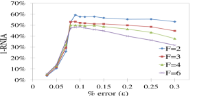
(c) Planted cluster: $\varepsilon$=0.1%, $F$=2.

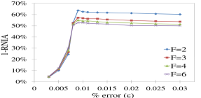
(d) Planted cluster: $\varepsilon$=0.01%, $F$=2.

Figure 11: The miner’s capability to capture fuzzy lagged co-clusters as a function of the miner’s settings of error and fuzziness (measured in terms of: $1\!-\!RNIA$).

Fig. 11 depicts the mining performance (measured in terms of: $1\!-\!RNIA$) of four different combinations of error and fuzziness of the planted clusters ($\varepsilon\!\in\!\{0.01\%,0.1\%\}$, $F\!\in\!\{2,4\}$) as a function of the miner’s configuration of error and fuzziness. Obviously the cluster in each configuration can be mined only if the fuzziness used by the miner is greater than or equal to the maximal fuzziness allowed when constructing the planted cluster. Therefore the miner’s fuzziness configuration was set to $F\geq 2$ in the case where the planted cluster was of maximum fuzziness of $2$ and $F\geq 4$ in the case of maximum fuzziness of $4$. The figure presents the average score over $100$ trials for each of the four combinations of the planted clusters’ parameters and for each configuration of the miner. The graphs demonstrate that, as expected, the best performances are achieved when the miner is set to the fuzziness of the planted cluster and to an error within the surrounding of the planted cluster. In addition, the higher the error or fuzziness to which the miner is set, the lower the performance achieved. This is due to increasing noise being added to the mined clusters. The charts in Fig. 11 are significant as they establish the importance of introducing fuzziness into the lagged-pattern model.

4.2 Experiments with Flight of Pigeon Flocks

In a second set of experiments, we examined the capability of the FLC algorithm to mine clusters from real-life data. One key goal for these experiments was to demonstrate the extent of improvement achieved in terms of mining coherency when transitioning from the lagged model to the fuzzy lagged model. For that purpose, we used two real-life datasets containing GPS readings of the flight of pigeon flocks [56] (see a snapshot in Fig. 12): (1) homing flight data, consisting of four different datasets recording the flights of pigeons from point A to point B; and (2) free flight data, consisting of 11 different datasets recording the flights of pigeons around the home loft, i.e., flight from point A back to point A. Each dataset (four of homing flight and 11 of free flight) represents a different flock release, containing an average of nine individuals.

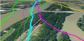
(a) homing flight

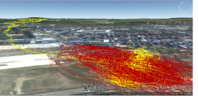
(b) free flight and homing flight

Figure 12: Snapshot of the homing flight and free flight datasets. Each line represents a pigeon’s trajectory. Pigeons belonging to the same flock are painted in the same color. The figures illustrate the presence of interleaving trajectories and therefore the difficulty in mining clusters which only contain pigeons of the same flock. These datasets present a serious challenge to mining algorithms (e.g., density-based algorithms such as DBSCAN [20], see Expt. 4.2.2 and 4.2.1), as well as to humans (see Expt. 4.2.2).

Generally speaking, a flock’s flight formation is a lagged pattern where the lag is the distance between the fliers. Nevertheless, clustering the pigeons according to their flock membership is not a trivial task. The trajectories of the flock members depend on multiple parameters: flier (e.g., physical ability, navigation capabilities, leader-follower relationships, threats) and weather conditions (e.g., wind streams, temperature). Many of these parameters change dramatically over time and space. The data are inherently noisy due to human error and equipment inaccuracy (e.g., GPS errors$/$inaccuracies$/$distortion, loss of signal, device failure). A further complication in the dataset is that flight trajectories are spatially close and highly interleaved. This is caused by the fact that flocks were all released (at different times) from a similar location heading to the same destination. For example, the homing flight pigeons followed the Danube river for about 15km until reaching their loft. This lack of spatial differentiation imposes a great mining challenge, especially to density-based algorithms, which might mistakenly merge trajectories that belong to different flocks. Therefore, mining such datasets for fuzzy lagged co-clusters is highly complex.

In the following experiments, we consider a cluster to be accurate if all the participating pigeons belong to the same flock. We note that it is unlikely to mine a cluster containing all pigeons in the flock as it is fairly common for pigeons to deviate from their flock for a substantial period of the flight (e.g., during flight no.3, two birds broke away from the group soon after release). Thus, such deviating pigeons cannot be accurately clustered.

4.2.1 Mixed Datasets: Homing Flight and Free Flight

The goal of the experiment is to test the error and fuzziness impact on the precision and recall of the mined clusters. To do so, we use a dataset compiled from mixed pairs of a homing flight and a free flight dataset (we compile $44$ different pairs of datasets which are the result of four homing flights and $11$ free flights dataset combinations, see example in Fig. 12b). We ran the FLC algorithm on each pair of datasets with various errors $\varepsilon$$\in$[0.005%–0.5%] and fuzziness $F$$\in$[0–10] combinations, recording the F₁ score of the mined clusters. In addition, we ran the DBSCAN algorithm [20] in order to compare its results to the FLC algorithm. The DBSCAN algorithm has two main parameters: (1) distance, denoted $Eps$, which represents the maximum neighborhood of a point; and (2) density, denoted $MinPts$, which represents the minimum number of points within the neighborhood of a point. The DBSCAN algorithm was run on each pair of datasets, with various combinations of distance $Eps$$\in$[0.001–10000] and density $MinPts$$\in$[2–10000], recording the F₁ score of the mined clusters.

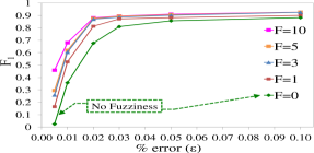
(a) FLC: F₁ vs. %error ($\varepsilon$).

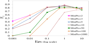
(b) DBSCAN: F₁ vs. distance ($Eps$).

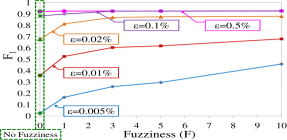
(c) FLC: F₁ vs. fuzziness ($F$).

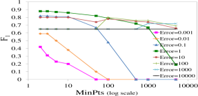
(d) DBSCAN: F₁ vs. density ($MinPts$).

Figure 13: F₁ score comparison of the FLC and DBSCAN algorithms. On the left, Fig. 13a and Fig. 13c depict the F₁ score as obtained by the FLC algorithm as a function of the error ($\varepsilon$) and fuzziness ($F$), respectively. On the right, Fig. 13b and Fig. 13d depict the F₁ score as obtained by the DBSCAN algorithm as a function of the distance ($Eps$) and density ($MinPts$), respectively.

Fig. 13a and 13c depict the F₁ score of the FLC algorithm as a function of the error ($\varepsilon$) and fuzziness ($F$), respectively. $F$=0 is in fact the case of mining lagged clusters with no fuzziness. As expected, any increase in $\varepsilon$ or $F$ results in an increase in the F₁ score as more data points are reachable from the cluster’s seed. An important finding obtained from the figures is that for relatively low errors, a significant increase in the F₁ score is recorded when fuzziness is used. For example, for $\varepsilon$=0.005%, we obtain for $F$={0, 1, 3, 5, 10} a score of F₁={0.024, 0.164, 0.259, 0.295, 0.458}, which reflects an increase of a factor of $\times$={1, 7, 10, 12, 19}, respectively. Figures 13b and 13d depict the equivalent performance of DBSCAN for the same settings (i.e., F₁ score as a function of the distance ($Eps$) and density ($MinPts$), respectively) used for generating figures 13a and 13c. Comparison of the FLC and DBSCAN algorithms reveals the stability of setting the FLC parameters vs. the sensitivity of configuring the DBSCAN parameters (surveyed in [12, 32]). In addition, even when considering the best configuration for the DBSCAN algorithm, the FLC algorithm still outperforms the best F₁ score achieved with DBSCAN. The comparison of Fig. 13a and Fig. 13b reveals the difference in the error (distance) behavior between the FLC and DBSCAN algorithms, respectively (note: the DBSCAN uses an Euclidean distance measure ($L_{2}$ norm), while the FLC uses the Manhattan distance measure ($L_{1}$ norm)). While the FLC algorithm maintains a high F₁ score as the error increases, the DBSCAN algorithm results in mining futile clusters of F₁=0.66 containing the entire dataset (the datasets used contain two classes with an equal number of members. Therefore, a cluster containing the entire dataset, will have a recall=1.0, precision=0.5 and thus F₁=0.66). The comparison of Fig. 13c and Fig. 13d reveals that while the fuzziness parameter of the FLC algorithm steadily increases the achieved F₁ score, the effect of the density parameter of the DBSCAN algorithm is not conclusive and depends on the adjacent error value.

The latter finding strengthens the importance and necessity of the fuzzy lagged model. The mining of non-fuzzy lagged co-clusters achieves a substantially lower F₁ score in comparison to the mining of fuzzy lagged co-clusters. Indeed, an increase in the F₁ measure can also be achieved by increasing the error $\varepsilon$; however, this is dangerous as any increase in $\varepsilon$ substantially increases the chance of mining artifacts. In addition, the increase in error may not always achieve a high F₁ score. For example, datasets with large spatial distances between the data points would require an error so large that it might cover the entire dataset, which in turn results in futile clusters. On the other hand, the use of fuzziness as part of the model, enables mining accurate and coherent clusters without increasing the allowable error. In addition, as illustrated in Fig. 13, a score close to $1$ for F₁ can be obtained even when considering moderate fuzziness.

4.2.2 Homing Flight Dataset

In order to examine the algorithm’s ability to properly classify each pigeon to its flock, we merged all four homing flight datasets resulting in a matrix of size $[37\times 13892]$, comprising 13892 GPS readings of 37 pigeons.

To demonstrate the difficulty of clustering the dataset into flocks (i.e., specifying how many flocks are present) we conducted the following experiment. We asked $25$ people, of differing sex, age, occupation and nationality, to specify how many flocks they could identify in the dataset. For that purpose, we enabled them to use Google Earth to view the pigeons’ trajectories (see Fig. 14 for sample snapshots of the user view). The subjects could use all functionalities within Google Earth (e.g., view the trajectories from different angles, enlarge, and so on), and were given $5$-minute to reach an answer. The average answer was $6.5$, with a standard deviation of $3.2$. Only $16\%$ of the subjects gave the correct answer (i.e., $4$ flocks). The results indicate that the dataset cannot be trivially mined.

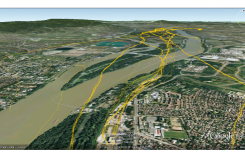
(a)

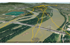
(b)

Figure 14: Snapshots of a user view of the homing flight dataset. The user was asked to specify the number of flocks (the correct answer is four).

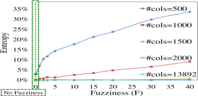
(a) Entropy vs. fuzziness.

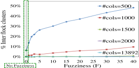
(b) Inter-flock vs. fuzziness.

Figure 15: Confusions of the mined clusters. Fig. 15a presents the entropy, while Fig. 15b presents the percentage of inter-flock clusters, i.e., clusters containing pigeons of different flocks. The lower the percentage, the higher the accuracy of the cluster.

To examine how many flocks the FLC algorithm would specify, we conducted the following experiment. We ran the FLC algorithm with an error set to $\varepsilon$=0.005% (following Fig. 13c, this error setting would enable the examination of the fuzziness effect) and various values of fuzziness $F$$\in${0, 1, 2, 3, 5, 10, 15, 20, 30, 40} for 20,000 trials. In addition, we wished to examine whether the use of partial knowledge (i.e., partial dataset), which necessarily reduces the overall mining run-time, would preserve the quality of the mining results. To do so, each of the above settings was run on various datasets comprising 4%, 7%, 11%, 14% and 100% of the dataset’s columns (500, 1000, 1500, 2000 and 13892 of dataset’s columns, respectively). Fig. 15 depicts the accuracy of the mined fuzzy lagged co-clusters. Fig. 15a presents the entropy of the mined clusters as a function of the fuzziness $F$ and the number of columns. The entropy of a cluster $C$ is computed as: $H(C)=-\sum\nolimits_{i=1}^{k}p(i|C)\cdot\log(p(i|C))$ for $k$ class labels in cluster $C$. Ideally, a cluster $C$ should contain objects of only one class and thus, have a zero entropy. For a set of clusters, we take the average entropy weighted by the number of objects per cluster. For readability, we normalize the entropy to the range of 0% to 100% by dividing by the maximum entropy, i.e., $H(C)/\log(k)$ [6, 69]. Fig. 15b presents the percentage of inter-flock clusters, i.e., clusters which contain pigeons from different flocks, as a function of the fuzziness $F$ and the number of columns. As the results demonstrate, due to the interleaving of the pigeons’ trajectories, using a small number of columns does not supply enough data to discriminate between pigeons belonging to different flocks. The probability of an inter-flock cluster for small number of columns (i.e., less than 1000, which is 7% of the dataset columns) is high. On the other hand, when using a large enough number of columns (i.e., more than 10% of the dataset columns) the probability of mining an inter-flock cluster is insignificant, even with respect to a growing fuzziness. Although we do not claim the generality of this approach, this latter finding is important in the aspect of run-time, as also the use of a partial dataset yields promising results. Moreover, we can use a post-process procedure which merges clusters that share common objects (i.e., clusters that had at least one pigeon in common were merged). Thus, with a high probability, the merged clusters will represent the different flocks. Fig. 16 presents the number of flocks (as yielded by the post-process stage) as a function of the fuzziness $F$ and the number of columns.

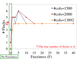
Figure 16: Number of flocks (as yielded by the post-process stage) as a function of the fuzziness and the number of columns. We notice that for $F$=0 (i.e., using the lagged co-clustering model) we do not obtain the correct answer (i.e., $4$), regardless of the number of columns being used. On the other hand, when using the fuzzy lagged co-clustering model, we quickly converge to the correct result, as the value of $F$ increases. Furthermore, we observe a quick convergence to the correct answer as the number of columns increases (e.g., for 13892 columns, we already obtain the correct result when using $F$=2).

We notice that for $F$=0 (i.e., using the lagged co-clustering model) we do not obtain the correct answer (i.e., four), regardless of the number of columns being used. On the other hand, when using the fuzzy lagged co-clustering model, we quickly converge to the correct result, as the value of $F$ increases. Furthermore, we observe a quick convergence to the correct answer as the number of columns increases (e.g., for 13892 columns, we already obtain the correct result when using $F$=2). As observed from the figure, the use of fuzziness led to the correct finding (four flocks) regardless of the number of columns used. Both the number of columns and the value of $F$ have a positive effect on the speed of convergence to the correct finding. In particular, with a large number of columns, only a very small level of fuzziness needs to be considered. In contrast, using the non-fuzzy model yielded on average only one group (one flock). As we next show, this is due to poor mining results as reflected by the coverage of $F$=0 in Fig. 17. Worth mentioning in this context is that human subjects gave an answer of (on average) 6.5 flocks.

A by-product of the post-process merging stage is the actual flock coverage, i.e., how many of the flock members have been covered by the mined clusters. Fig. 17 depicts the average flock coverage (over the numbers of columns$\in${1500, 2000, 13892}) for the homing flight dataset as a function of the fuzziness $F$.

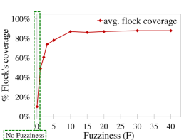
Figure 17: Average flock coverage vs. fuzziness for the homing flight dataset (we present only the average as the graphs for the various settings were insignificantly different). Compared to the non-fuzzy model, using the fuzzy model notably improves the coverage results. Even with the use of $F$=1, a substantial improvement is achieved in comparison to traditional methods that do not take the fuzziness into account (i.e., the regular lagged co-clustering approach). In this example, the improvement is from a coverage of 10% (with $F$=0) to a coverage of 50% with $F$=1. The use of higher fuzziness, e.g., $F$=40, brings the coverage up to $\sim$90%.

The results show a significant improvement in the accuracy and completeness of the mining process when using the fuzzy model ($F$$\geq$1) in comparison to the non-fuzzy model ($F$=0). Even the use of a fuzziness of a single column (i.e., $F$=1) has a notable impact of $\times$5 on the coverage. The use of high $F$, provides coverage of $\sim$90% of the flocks’ members.

To compare the performance of the FLC algorithm, we ran the DBSCAN algorithm [20] with various combinations of distance $Eps$$\in$[0.0001–10000] and density $MinPts$$\in$[2–500000].

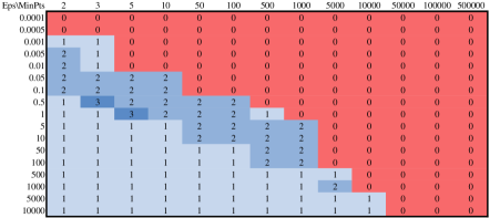
Figure 18: Number of flocks as obtained by the DBSCAN algorithm [20] as a function of the distance ($Eps$) and density ($MinPts$) as yielded by the post-process merging stage. Actual number of flocks is four.

Fig. 18 depicts the number of flocks as obtained by the DBSCAN algorithm (as yielded by the post-process stage) as a function of the distance and density used. For the vast majority of the settings, the DBSCAN algorithm either does not find any clusters (upper right portion – red color) or the clusters that it does find contain the entire dataset (lower left portion – blue color) and are therefore futile. Only for a negligible number of settings does the DBSCAN algorithm manage to report three flocks, which even then is not the correct answer of four. We note that the DBSCAN algorithm results as presented in Fig. 18 are based on a post-process merging stage, as the results without such a stage were considerably inferior. On the same range of settings as in Fig. 18, the obtained average number of flocks without the post-processing stage was $87$ with a standard deviation of $463$, where less than 0.5% of the settings yield the correct answer of $4$.

To summarize, mining this dataset is not a trivial task. This is evidenced by the poor classification results of the human subjects, the DBSCAN algorithm and the non-fuzzy lagged method. Furthermore, when using a non-fuzzy mining model, the obtained results are characterized by a low F₁ score and low coverage. On the other hand, the FLC algorithm performed well in mining fuzzy lagged co-clusters on various trajectories. It achieved a high F₁ score and high coverage, doing so with only a small number of artifact (inter-flock) clusters. Although prior domain knowledge can be useful in configuring the miner’s parameters, such knowledge is not mandatory. Subsection 3.3 provides default values for setting the parameters $|S|$ and $N$ (see Theorem 3.6 and 3.9, respectively). In order to choose an appropriate value of error, one can adopt any of the methods suggested for the non-fuzzy lagged co-clustering model [70], e.g., gradual increase, starting from a relatively small error. Setting the minimum cluster dimensions (i.e., $\beta$ and $\gamma$) to relatively small values would suffice for mining accurate clusters (e.g., $\beta$=2 and $\gamma$=10% as depicted by Fig. 15). When setting the fuzziness, the use of small values (e.g., $F$=1,2 as depicted by Fig. 16 and 17) already effects a considerable improvement in the clustering results over the non-fuzzy ones. In conclusion, the significant improvement in mining presented by the FLC algorithm, in comparison to the non-fuzzy algorithm, demonstrates the importance of including the fuzzy aspect in the model. The FLC algorithm can thus be used as a classifier in this domain.

5 Related Work

With the vast amount of routinely collected data, the need for clustering as a mining tool emerges in many fields: biology, physics, economics and computer science are but a short list of domains with a wealth of research in this direction [36, 47]. A typical mining problem is the extraction of patterns from a dataset, where the rows represent objects, the columns represent attributes and the data entries are the measurements of the objects over the attributes [36, 40].

Simple mining techniques look for a fully dimensional cluster: a subset of the objects over all attributes (or vice versa) [40, 64, 19, 71]. These techniques have several inherent vulnerabilities, e.g., difficulty in handling the common presence of irrelevant, noisy or missing attributes and inaccuracy due to the “curse of dimensionality” [10, 54, 72, 13, 45]. All these may be counter-productive as they increase background noise [40, 52].

Cheng and Church [17], in their seminal work in the field of gene expression data, introduced a mining technique which focus on mining biclusters (also known as co-clusters or co-regulations): a subset of the objects over a subset of the attributes. Their approach was followed by many researchers (see surveys by [52, 75, 54, 12, 40, 45]), using various models (additive vs. multiplicity, axis alignment, rows over columns preferment, cluster scoring function, overlapping, etc.), and applying various algorithmic strategies: greedy [17, 7], divide-and-conquer [33], projected clustering [49, 65], exhaustive enumeration [74], spectral analysis [43, 73], CTWC [22], bayesian networks [9], etc.

Due to the importance of datasets having a temporal nature (i.e., sequences of time series), specific efforts have been directed at utilizing the continuous nature of time as a natural order [39, 8, 38, 55], surveyed by [67, 81]. In particular, some have considered the delay (lag) between the object’s behaviors and suggested different approaches for mining lagged co-clusters. These include dynamic-programming and hierarchical-merging (with pruning) [85, 79], polynomial time Monte-Carlo strategies to mine lagged co-clusters which encompass the optimal lagged co-cluster [70], and the reduction to some finite alphabet [27]. Despite the efficiency of these approaches in mining lagged co-clusters, they become ineffective when the lagged pattern is fuzzy. This is due to their underlying assumption of non-noisy (i.e., fixed) lags.

Existing methods that are inherently designed for mining fuzzy lagged co-clusters can be categorized into three types, each imposing a different design limitation. The first is a group of methods designed for mining pairs of sequences using variants of the edit distance measures, such as the Longest Common Sub Sequence (LCSS) measure [78] and others [84, 16, 15], surveyed in [35]. However, post-processing merging requires a combinatorial solution which is both time consuming and heavily dependent on the closeness of the merit function [40, 71]. Furthermore, pairs of objects might lack the transitivity characteristic, e.g., two stocks may appear to be correlated, while in fact the correlation is to the index which dominates them in volatile trading days [71]. Investments based on this in nonvolatile times may lead to poor results. Moreover, pairs might simply be merged as a mere aggregation of noise and not due to some hidden regulatory mechanism [13, 70]. The second type uses a space reduction approach to some finite alphabet [26, 23, 2, 63, 62, 61, 37], e.g., each trajectory coordinate is approximated to a grid cell. The main limitation of such methods is the reduction magnitude. On one hand, coarse abstraction using a small alphabet may lead to greater errors and finer clusters being missed. On the other hand, using a large alphabet will have a dramatic influence on the run-time as it is exponentially dependent on the alphabet size. Finally, there are methods that assume sequentiality of the cluster’s columns, e.g., flock mining [48, 11].

A popular technique for mining clusters of trajectories is the density-based approach. This approach uses the spatial closeness between data points to associate them into clusters [31, 34, 61, 1]. A well known representative of this technique is the DBSCAN algorithm [20] (followed by derivative algorithms of a non-temporal [58, 3, 57, 86, 51, 76] and temporal [14, 68, 42, 48, 76] nature, surveyed in [12, 32]). The disadvantage of the density-based approach is its sensitivity to noise (e.g., signal distortion), outliers (e.g., erroneous GPS measurements), missing values (in real-life, devices may be voluntarily disconnected by their owners, or be subject to machine failures or lost signal), related objects which are spatially distant (e.g., a roaming group where members are far apart from each other) and crossing trajectories of unrelated objects (e.g., trajectories of different groups interleave). These algorithms will find the data used in Subsection 4.2 challenging as trajectories of different groups interleave. This may cause clusters to contain inter-group trajectories, and thus, fail classification.

We note that all the works cited above were also unable to find substantial previous reference to the fuzzy lagged co-clustering problem and that state-of-the art algorithms for this problem are either non-fuzzy [79, 70] or limited to data points which are spatially close [20].

On the application side, the last few years have witnessed an increasing interest in fuzzy lagged co-clustering. This is attributed to the dramatic increase in location-aware devices (e.g., cellular, GPS, RFID). Such devices leave behind spatio-temporal electronic trails. A dataset of such trajectories is of a fuzzy lagged nature. Commercial services such as Foursquare, Google Latitude, Microsoft GeoLife, and Facebook Places, use such data to maintain location-based social networks (LBSN), later used for personal marketing purposes. Another use of such data is to extract patterns (see surveys in [44, 32, 4]) which may suggest Places Of Interest (POI) [58, 42, 41, 26, 24]. This is mostly used for the purposes of tourism [25, 24, 26, 58, 5], urban planning [24, 26, 30], crowd control [26, 30], traffic management [58, 63, 62, 30] and behavioral sciences [21, 80, 46].

6 Discussion, Conclusions and Future Work

The importance of clustering is unquestionable and has been thoroughly discussed and demonstrated in cited prior work. Similarly, the extensive co-clustering literature includes many examples of the benefit of mining co-clusters as opposed to traditional approaches. The fuzzy lagged co-cluster model generalizes the lagged co-cluster model, enabling the inclusion of an additional important dimension, a fuzzy aspect, in the regulatory paradigm. The results reported in the previous section not only corroborate the algorithm’s ability to efficiently mine relevant and accurate fuzzy lagged co-clusters, but also illustrate the importance of including fuzziness in the lagged-pattern model. With the fuzziness dimension, a significant improvement is achieved in both coverage and F₁ measures in comparison to using the regular lagged co-clustering model. One important strength of the new model relates to the chance of mining artifacts. In order to enlarge the dimensions of the mined clusters, traditional non-fuzzy methods tend to increase the error which in turn increases the risk of mining artifacts. The fuzzy model provides the user with the capability of keeping a low level of error, while improving the achieved performance, without introducing artifacts.

As proved in Subsection 2.1, the complexity of mining fuzzy lagged co-clusters is NP-complete for most interesting optimality measures. Thus the importance of the algorithm presented in this paper lies in promising the probability of mining an optimal fuzzy lagged co-cluster and a theoretical bound to the polynomial number of iterations it will take. In addition, the algorithm demonstrates a set of important capabilities such as handling noise, missing values, anti-correlations and overlapping patterns. Moreover, even if lagged clusters with no fuzziness at all need to be mined, the FLC algorithm has a better run-time in comparison to former algorithms inherently designed for such cases [85, 79] (including the Monte-Carlo based algorithms [70]). It is notable that due to the Monte-Carlo nature of the FLC algorithm, its iterations (and therefore, the mined clusters) are independent of each other. The algorithm can thus be implemented to take advantage of parallel computing or special hardware in a straightforward manner.

The experiments using an artificial environment (reported in the previous section) reveal actual performance which is far better, in terms of accuracy and efficiency, than the theoretical bounds. In addition, they supply default values for the various configurable parameters of the algorithm, releasing the user from this burden. When used on real-life datasets, the FLC algorithm was demonstrated to mine precise, coherent and relevant fuzzy lagged co-clusters in a practicable run-time and with almost no artifacts. This is in contrast to inferior results obtained by using a non-fuzzy model and despite the fact the datasets were large, highly noisy, contained many missing values, and were rich in overlapping clusters. In addition, the FLC algorithm presented classification capabilities which were superior to the ones presented by the non-fuzzy lagged model, those of human subjects and to the DBSCAN algorithm. This encouraging result is important in the sense of model validation and suggests great potential for mining fuzzy lagged co-clusters in many other fields of science, business, technology and medicine.

As in the non-fuzzy lagged model, the ability of the FLC algorithm to mine lagged co-clusters offers important functionalities such as forecasting. However, when mining fuzzy lagged co-clusters, one may have to choose between possibly intersecting columns (see Subsection 3.4.3). One can utilize the intersecting mechanism to place weights on the matrix columns so as to enable the mining of more “recent” clusters. It is reasonable to assume that the latest (up-to-date) columns will contribute more to the accuracy of the forecast than old and possibly irrelevant ones. We believe there is far more that can be developed in this aspect in terms of future research.

Author Biographies

Eran Shaham In 1998, Eran Shaham received his B.Sc. degree in Mathematics and Computer Science from Ben-Gurion University, Israel. From 1999 to 2001, he worked at Parametric Technology Corporation (PTC), Israel. In 2004, he received his M.Sc. degree in Computer Science from Ben-Gurion University, Israel. From 2005 to 2008, he worked at the IBM Haifa Research Lab, Israel. He is currently a Ph.D. student at the Department of Computer Science, Bar-Ilan University, Israel. His research interests include data mining in general and its lagged aspects in particular.

David Sarne David Sarne is a senior lecturer in the Computer Science department in Bar-Ilan University, Israel. He received a B.Sc., M.Sc., and a Ph.D. degree in Computer Science from Bar-Ilan University, Israel. During 2005-2007 he was a post-doctoral fellow at Harvard University. His research interests include economic search theory, market mechanisms for forming cooperation (mechanism design) and multi-agent systems.

Boaz Ben-Moshe Boaz Ben-Moshe is a faculty member in the Department of Computer in Ariel University, Israel. He received the B.Sc., M.Sc., and Ph.D. degrees in Computer Science from Ben-Gurion University, Israel. During 2004-2005 he was a post-doctoral fellow at Simon Fraser University, Vancouver, Canada. His main research areas are: Computational Geometry and GIS algorithms. His research includes Geometric data compression, Optimization of wireless networks, Computing visibility graphs, and Vehicle routing problems. In 2008 he has founded the Kinematics and Computational Geometry Laboratory with Dr. Nir Shvalb, see: http://www.ariel.ac.il/sites/kcg.

Table: Notations used and their meaning.

Notation	Meaning
$m$	number of rows
$n$	number of columns
$X$	real number matrix of size $m\times n$
$I$	a subset of the rows, i.e., $I\subseteq m$
$T$	the corresponding lags of the rows in $I$ ($|T|=|I|$)
$J$	a subset of the columns, i.e., $J\subseteq n$
$F$	maximal fuzziness degree
$(I,T,J,F)$	a fuzzy lagged co-cluster of matrix $X$
$f_{i,j}$	the fuzzy alignment of object $i$ to sample $j$,
	i.e., $-F\leq f_{i,j}\leq F$, for all $i\in I$ and $j\in J$
$G_{i}$	a latent variable indicating object $i$’s regulation strength
$H_{j}$	a latent variable indicating the regulatory intensity of sample $j$
$\eta$	relative error
$A$	$X$ logarithm transformation, i.e., $A_{i,j}=\log(X_{i,j})$
$\varepsilon$	$\eta$ logarithm transformation, i.e., $\varepsilon=\log(\eta)$
$R_{i}$	$G_{i}$ logarithm transformation, i.e., $R_{i}=\log(G_{i})$
$C_{j}$	$H_{j}$ logarithm transformation, i.e., $C_{j}=\log(H_{j})$
$\mu(I,J)$	objective function of a cluster
$\varepsilon_{{}_{T,F}}(I,J)$	an error of a fuzzy lagged co-cluster
$\beta$	minimum number of the rows, expressed as a fraction of $m$
$\gamma$	minimum number of the columns, expressed as a fraction of $n$
$p$	discriminating row ($p\in I$)
$s$	discriminating column ($s\in J$)
$S$	discriminating column set ($S\subseteq J$)
$S^{0}$	a subset of $S$ having zero fuzziness over all cluster’s rows
$N$	number of iterations the FLC algorithm runs

Eran Shaham, Department of Computer Science, Bar-Ilan University, Ramat-Gan, 52900 Israel. Email: erans@macs.biu.ac.il.

References

- [1] G. Al-Naymat, S. Chawla, and J. Gudmundsson. Dimensionality reduction for long duration and complex spatio-temporal queries. In Symposium on Applied computing, pages 393–397, 2007.
- [2] L. Alvares, V. Bogorny, B. Kuijpers, J. de Macedo, B. Moelans, and A. Vaisman. A model for enriching trajectories with semantic geographical information. In International symposium on advances in geographic information systems, pages 1–8, 2007.
- [3] M. Ankerst, M. M. Breunig, H. P. Kriegel, and J. Sander. OPTICS: ordering points to identify the clustering structure. In International conference on Management of Data, pages 49–60, 1999.
- [4] C. Antunes and A. Oliveira. Temporal data mining: an overview. In KDD Workshop on Temporal Data Mining, pages 1–15, 2001.
- [5] Y. Asakura and T. Iryo. Analysis of tourist behaviour based on the tracking data collected using a mobile communication instrument. Transportation Research Part A: Policy and Practice, 41(7):684–690, 2007.
- [6] I. Assent, R. Krieger, E. Muller, and T. Seidl. DUSC: Dimensionality Unbiased Subspace Clustering. In International Conference on Data Mining, pages 409–414, 2007.
- [7] W. Ayadi, M. Elloumi, and J. Hao. BicFinder: a biclustering algorithm for microarray data analysis. Knowledge and Information Systems, pages 1–18, 2011.
- [8] Z. Bar-Joseph, D. Gifford, T. Jaakkola, and I. Simon. A new approach to analyzing gene expression time series data. In International conference on computational biology, pages 39–48, 2002.
- [9] Y. Barash and N. Friedman. Context-specific Bayesian clustering for gene expression data. Computational Biology, 9(2):169–191, 2002.
- [10] R. Bellman. Dynamic Programming. Science, 153(3731):34–37, 1966.
- [11] M. Benkert, J. Gudmundsson, F. Hubner, and T. Wolle. Reporting flock patterns. Computational Geometry, 41(3):111–125, 2008.
- [12] P. Berkhin. A survey of clustering data mining techniques. Grouping Multidimensional Data, pages 25–71, 2006.
- [13] K. Beyer, J. Goldstein, R. Ramakrishnan, and U. Shaft. When is “nearest neighbor” meaningful? Database Theory, pages 217–235, 1999.
- [14] D. Birant and A. Kut. ST-DBSCAN: An algorithm for clustering spatial-temporal data. Data and Knowledge Engineering, 60(1):208–221, 2007.
- [15] L. Chen and R. Ng. On the marriage of lp-norms and edit distance. In International conference on Very large data bases, pages 792–803, 2004.
- [16] L. Chen, M. TamerOzsu, and V. Oria. Robust and fast similarity search for moving object trajectories. In International conference on Management of data, pages 491–502, 2005.
- [17] Y. Cheng and G. M. Church. Biclustering of expression data. In International Conference on Intelligent Systems for Molecular Biology, pages 93–103, 2000.
- [18] S. Diliberto and E. Straus. On the approximation of a function of several variables by the sum of functions of fewer variables. Pacific Journal of Mathematics, 1(2):195–210, 1951.
- [19] S. Erdal, O. Ozturk, D. Armbruster, H. Ferhatosmanoglu, and W. Ray. A time series analysis of microarray data. In Symposium on bioinformatics and bioengineering, pages 366–378, 2004.
- [20] M. Ester, H. Kriegel, J. Sander, and X. Xu. A Density-Based Algorithm for Discovering Clusters in Large Spatial Databases with Noise. In International Conference on Knowledge Discovery and Data mining, pages 226–231, 1996.
- [21] D. Forsyth. Group dynamics. Wadsworth Pub Co, 2009.
- [22] G. Getz, E. Levine, and E. Domany. Coupled two-way clustering analysis of gene microarray data. National Academy of Sciences, 97(22):12079–12084, 2000.
- [23] F. Giannotti, M. Nanni, F. Pinelli, and D. Pedreschi. Trajectory pattern mining. In International conference on knowledge discovery and data mining, pages 330–339, 2007.
- [24] F. Girardin, F. Calabrese, F. Fiore, C. Ratti, and J. Blat. Digital footprinting: Uncovering tourists with user-generated content. Pervasive Computing, 7(4):36–43, 2008.
- [25] F. Girardin, F. Fiore, C. Ratti, and J. Blat. Leveraging explicitly disclosed location information to understand tourist dynamics: a case study. Location Based Services, 2(1):41–56, 2008.
- [26] F. Girardin, A. Vaccari, A. Gerber, and C. Ratti. Quantifying urban attractiveness from the distribution and density of digital footprints. Spatial Data Infrastructure Research, 4:175–200, 2009.
- [27] J. P. Gonçalves and S. C. Madeira. Heuristic approaches for time-lagged biclustering. In International Workshop on Data Mining in Bioinformatics, pages 1–9, 2013.
- [28] M. Grötschel, L. Lovász, and A. Schrijver. Polynomial algorithms for perfect graphs. Annals of Discrete Mathematics, 21:325–356, 1984.
- [29] M. Grötschel, L. Lovász, and A. Schrijver. Geometric Algorithms and Combinatorial Optimization. Springer, 1988.
- [30] J. Gudmundsson, P. Laube, and T. Wolle. Movement patterns in spatio-temporal data. Encyclopedia of GIS, pages 726–732, 2008.
- [31] J. Gudmundsson, M. van Kreveld, and B. Speckmann. Efficient detection of patterns in 2D trajectories of moving points. Geoinformatica, 11(2):195–215, 2007.
- [32] J. Han, M. Kamber, and A. Tung. Spatial Clustering Methods in Data Mining: A Survey. Geographic Data Mining and Knowledge Discovery, pages 33–50, 2001.
- [33] J. Hartigan. Direct clustering of a data matrix. Journal of the American Statistical Association, pages 123–129, 1972.
- [34] S. Hwang, Y. Liu, J. Chiu, and E. Lim. Mining mobile group patterns: A trajectory-based approach. Advances in Knowledge Discovery and Data Mining, pages 145–146, 2005.
- [35] Y. Ishikawa. Data Mining for Moving Object Databases. Mobile Intelligence, pages 237–263, 2010.
- [36] A. K. Jain, M. N. Murty, and P. J. Flynn. Data clustering: a review. ACM computing surveys, 31(3):264–323, 1999.
- [37] L. Ji and K. Tan. Identifying time-lagged gene clusters using gene expression data. Bioinformatics, 21(4):509–516, 2005.
- [38] D. Jiang, J. Pei, M. Ramanathan, C. Tang, and A. Zhang. Mining coherent gene clusters from gene-sample-time microarray data. In International conference on knowledge discovery and data mining, pages 430–439, 2004.
- [39] D. Jiang, J. Pei, and A. Zhang. Interactive exploration of coherent patterns in time-series gene expression data. In International conference on Knowledge discovery and data mining, pages 565–570, 2003.
- [40] D. Jiang, C. Tang, and A. Zhang. Cluster analysis for gene expression data: A survey. Transactions on Knowledge and Data Engineering, 16(11):1370–1386, 2004.
- [41] S. Kisilevich, D. Keim, and L. Rokach. A novel approach to mining travel sequences using collections of geotagged photos. Geospatial Thinking, pages 163–182, 2010.
- [42] S. Kisilevich, M. Krstajic, D. Keim, N. Andrienko, and G. Andrienko. Event-Based Analysis of People’s Activities and Behavior Using Flickr and Panoramio Geotagged Photo Collections. In International conference Information Visualisation, pages 289–296, 2010.
- [43] Y. Kluger, R. Basri, J. T. Chang, and M. Gerstein. Spectral biclustering of microarray data: coclustering genes and conditions. Genome Research, 13(4):703–716, 2003.
- [44] K. Koperski, J. Adhikary, and J. Han. Spatial data mining: progress and challenges survey paper. In Workshop on Research Issues on Data Mining and Knowledge Discovery, pages 55–70, 1996.
- [45] H. P. Kriegel, P. Kröger, and A. Zimek. Clustering high-dimensional data: A survey on subspace clustering, pattern-based clustering, and correlation clustering. ACM Transactions on Knowledge Discovery from Data, 3(1):1–58, 2009.
- [46] H. Lauw, E. Lim, T. Tan, and H. Pang. Mining social network from spatio-temporal events. In Workshop on Link Analysis, Counterterriorism and Security, pages 82–93, 2005.
- [47] S. Laxman and P. Sastry. A survey of temporal data mining. Sadhana, 31(2):173–198, 2006.
- [48] J. Lee, J. Han, and K. Whang. Trajectory clustering: a partition-and-group framework. In International conference on Management of data, pages 593–604, 2007.
- [49] S. Lonardi, W. Szpankowski, and Q. Yang. Finding biclusters by random projections. Theoretical Computer Science, 368(3):217–230, 2006.
- [50] L. Lovász. Normal hypergraphs and the perfect graph conjecture. Discrete Mathematics, 2(3):253–267, 1972.
- [51] D. Ma and A. Zhang. An adaptive density-based clustering algorithm for spatial database with noise. In International Conference on Data Mining, pages 467–470, 2004.
- [52] S. C. Madeira and A. L. Oliveira. Biclustering algorithms for biological data analysis: a survey. Transactions on Computational Biology and Bioinformatics, 1(1):24–45, 2004.
- [53] A. A. Melkman and E. Shaham. Sleeved CoClustering. In Knowledge discovery and data mining, pages 635–640, 2004.
- [54] G. Moise, A. Zimek, P. Kroeger, H. Kriegel, and J. Sander. Subspace and projected clustering: experimental evaluation and analysis. Knowledge and Information Systems, 21(3):299–326, 2009.
- [55] C. Moller-Levet, F. Klawonn, K. Cho, H. Yin, and O. Wolkenhauer. Clustering of unevenly sampled gene expression time-series data. Fuzzy sets and Systems, 152:49–66, 2005.
- [56] M. Nagy, Z. Ákos, D. Biro, and T. Vicsek. Hierarchical group dynamics in pigeon flocks. Nature, 464(7290):890–893, 2010.
- [57] R. Ng and J. Han. Efficient and effective clustering methods for spatial data mining. In International conference on Very Large Data Bases, pages 144–144, 1994.
- [58] A. Palma, V. Bogorny, B. Kuijpers, and L. Alvares. A clustering-based approach for discovering interesting places in trajectories. In Symposium on Applied computing, pages 863–868, 2008.
- [59] A. Patrikainen and M. Meila. Comparing subspace clusterings. Transactions on Knowledge and Data Engineering, 18(7):902–916, 2006.
- [60] R. Peeters. The maximum edge biclique problem is NP-complete. Discrete Applied Mathematics, 131(3):651–654, 2003.
- [61] N. Pelekis, I. Kopanakis, E. Kotsifakos, E. Frentzos, and Y. Theodoridis. Clustering trajectories of moving objects in an uncertain world. In International Conference on Data Mining, pages 417–427, 2009.
- [62] N. Pelekis, I. Kopanakis, E. Kotsifakos, E. Frentzos, and Y. Theodoridis. Clustering uncertain trajectories. Knowledge and Information Systems, pages 1–31, 2010.
- [63] N. Pelekis, I. Kopanakis, C. Panagiotakis, and Y. Theodoridis. Unsupervised trajectory sampling. Machine Learning and Knowledge Discovery in Databases, pages 17–33, 2010.
- [64] V. Plerou, P. Gopikrishnan, B. Rosenow, L. A. N. Amaral, and H. E. Stanley. Universal and nonuniversal properties of cross correlations in financial time series. Physical Review Letters, 83(7):1471–1474, 1999.
- [65] C. M. Procopiuc, M. Jones, P. K. Agarwal, and T. Murali. A Monte Carlo algorithm for fast projective clustering. In International conference on Management of Data, pages 418–427, 2002.
- [66] N. Robertson, R. Thomas, M. Chudnovsky, and P. Seymour. The strong perfect graph theorem. Annals of mathematics, 164(1):51–229, 2006.
- [67] J. Roddick and M. Spiliopoulou. A survey of temporal knowledge discovery paradigms and methods. Transactions on Knowledge and data engineering, 14(4):750–767, 2002.
- [68] J. Sander, M. Ester, H. Kriegel, and X. Xu. Density-Based Clustering in Spatial Databases: The Algorithm GDBSCAN and its Applications. Data Mining and Knowledge Discovery, 2(2):169–194, 1998.
- [69] K. Sequeira and M. Zaki. SCHISM: A New Approach to Interesting Subspace Mining. In International Conference on Data Mining, pages 186–193, 2004.
- [70] E. Shaham, D. Sarne, and B. Ben-Moshe. Sleeved co-clustering of lagged data. Knowledge and Information Systems, 31(2):251–279, 2012.
- [71] Y. Shapira, D. Kenett, and E. Ben-Jacob. The index cohesive effect on stock market correlations. European Physical Journal B-Condensed Matter and Complex Systems, 72(4):657–669, 2009.
- [72] Y. Shi and L. Zhang. COID: A cluster–outlier iterative detection approach to multi-dimensional data analysis. Knowledge and Information Systems, 28(3):709–733, 2011.
- [73] B. Takacs and Y. Demiris. Spectral clustering in multi-agent systems. Knowledge and information systems, 25(3):607–622, 2010.
- [74] A. Tanay, R. Sharan, and R. Shamir. Discovering statistically significant biclusters in gene expression data. Bioinformatics, 18(1):136–144, 2002.
- [75] A. Tanay, R. Sharan, and R. Shamir. Biclustering algorithms: A survey. Handbook of computational molecular biology, 9:1–261, 2005.
- [76] M. Tang, Y. Zhou, J. Li, W. Wang, P. Cui, Y. Hou, Z. Luo, J. Li, F. Lei, and B. Yan. Exploring the wild birds migration data for the disease spread study of H5N1: a clustering and association approach. Knowledge and Information Systems, 27(2):227–251, 2011.
- [77] C. Van Rijsbergen. Information retrieval. Butterworths, 2nd edition, 1979.
- [78] M. Vlachos, D. Gunopoulos, and G. Kollios. Discovering similar multidimensional trajectories. In International conference on data engineering, pages 673–684, 2002.
- [79] G. Wang, Y. Zhao, X. Zhao, B. Wang, and B. Qiao. Efficiently mining local conserved clusters from gene expression data. Neurocomputing, 73(7):1425–1437, 2010.
- [80] Y. Wang, E. Lim, and S. Hwang. Efficient mining of group patterns from user movement data. Data and Knowledge Engineering, 57(3):240–282, 2006.
- [81] T. Warren Liao. Clustering of time series data - a survey. Pattern Recognition, 38(11):1857–1874, 2005.
- [82] Wolfram Alpha LLC, access Feb 18, 2012.
- [83] J. Yang, H. Wang, W. Wang, and P. Yu. Enhanced biclustering on expression data. In Bioinformatics and Bioengineering, pages 321–327, 2003.
- [84] B. Yi, H. Jagadish, and C. Faloutsos. Efficient retrieval of similar time sequences under time warping. In International Conference on Data Engineering, pages 201–208, 1998.
- [85] Y. Yin, Y. Zhao, B. Zhang, and G. Wang. Mining time-shifting co-regulation patterns from gene expression data. In Advances in Data and Web Management, pages 62–73, 2007.
- [86] C. Zhou, D. Frankowski, P. Ludford, S. Shekhar, and L. Terveen. Discovering personally meaningful places: An interactive clustering approach. Transactions on Information Systems, 25(3):1–31, 2007.