The DiskMass Survey. VIII.
On the Relationship Between Disk Stability and Star Formation

Abstract

We study the relationship between the stability level of late-type galaxy disks and their star-formation activity using integral-field gaseous and stellar kinematic data. Specifically, we compare the two-component (gas$+$stars) stability parameter from Romeo & Wiegert ($Q_{\rm RW}$), incorporating stellar kinematic data for the first time, and the star-formation rate estimated from 21cm continuum emission. We determine the stability level of each disk probabilistically using a Bayesian analysis of our data and a simple dynamical model. Our method incorporates the shape of the stellar velocity ellipsoid (SVE) and yields robust SVE measurements for over 90% of our sample. Averaging over this subsample, we find a meridional shape of $\sigma_{z}/\sigma_{R}=0.51^{+0.36}_{-0.25}$ for the SVE and, at 1.5 disk scale lengths, a stability parameter of $Q_{\rm RW}=2.0\pm 0.9$. We also find that the disk-averaged star-formation-rate surface density ($\dot{\Sigma}_{e,\ast}$) is correlated with the disk-averaged gas and stellar mass surface densities ($\Sigma_{e,g}$ and $\Sigma_{e,\ast}$) and anti-correlated with $Q_{\rm RW}$. We show that an anti-correlation between $\dot{\Sigma}_{e,\ast}$ and $Q_{\rm RW}$ can be predicted using empirical scaling relations, such that this outcome is consistent with well-established statistical properties of star-forming galaxies. Interestingly, $\dot{\Sigma}_{e,\ast}$ is not correlated with the gas-only or star-only Toomre parameters, demonstrating the merit of calculating a multi-component stability parameter when comparing to star-formation activity. Finally, our results are consistent with the Ostriker et al. model of self-regulated star-formation, which predicts $\dot{\Sigma}_{e,\ast}/\Sigma_{e,g}\propto\Sigma_{e,\ast}^{1/2}$. Based on this and other theoretical expectations, we discuss the possibility of a physical link between disk stability level and star-formation rate in light of our empirical results.

1. Introduction

Stars are formed by the collapse of gas. In galaxy disks, a gas cloud should be gravitationally unstable if (1) it cannot adjust its internal pressure to balance the local gravitational pressure on timescales shorter than a free-fall time and (2) it occupies an area smaller than the scale on which differential rotation will shear it apart. Toomre (1964) codified these concepts into a criterion for the stability of an infinitely thin, rotating, self-gravitating, fluid disk:

$$Q=\frac{\kappa\sigma}{\pi G\Sigma}>1,$$ (1)

where

$$\kappa^{2}=2\frac{v_{c}}{R}\left(\frac{v_{c}}{R}+\frac{\partial v_{c}}{\partial R}\right)$$ (2)

is the epicyclic frequency, $v_{c}$ is the circular speed of the potential, $\sigma$ is the radial velocity dispersion, $\Sigma$ is the mass surface density, and $G$ is the gravitational constant. However, self-gravity is only one major player in the star-formation process, with chemodynamical processes, turbulence, and magnetic fields also significantly affecting the dynamics (see McKee & Ostriker, 2007, and references therein). The relative importance of these physical properties to the star-formation law is a matter of ongoing debate.

Empirical studies of the star-formation law in disk galaxies have predominantly focused on observations of their gaseous components. In a seminal article, Kennicutt (1998, hereafter K98) demonstrated that the star-formation rate per unit area ($\Sigma_{\rm SFR}$), or equivalently the time derivative of the stellar mass surface density ($\dot{\Sigma}_{\ast}\equiv\Sigma_{\rm SFR}$), is well correlated with the surface density of the hydrogen gas, $\Sigma_{\rm H}=\Sigma_{\mbox{\rm\footnotesize H{i}}}+\Sigma_{\rm H_{2}}$, following the star-formation law suggested by Schmidt (1959). Considering the proportionality from equation 1, one might expect such a relation if star-formation is driven by self-gravity. Owing much to the flood of relevant data, the quantitative details of the star-formation law in galaxy disks and its relation to the Kennicutt-Schmidt (KS) law ($\dot{\Sigma}_{\ast}\propto\Sigma_{\rm H}^{1.4}$; K98, ) have been greatly scrutinized. This scrutiny has lead to a number of alternatives to this paradigm; see compilations by, e.g., Leroy et al. (2008) and Zheng et al. (2013).

Many of these alternatives involve consideration of gas properties, such as accounting for the dust-to-gas ratio (Leroy et al., 2013), or use of specific gas tracers. Wong & Blitz (2002) and Bigiel et al. (2008) have shown that $\dot{\Sigma}_{\ast}$ is more tightly correlated with $\Sigma_{\rm H_{2}}$ than with $\Sigma_{\rm H}$. Therefore, the star-formation law will also be affected by the ability of the interstellar medium to convert H i to H₂ (Blitz & Rosolowsky, 2004, 2006), which can be related to the hydrostatic pressure in the disk plane (Elmegreen, 1989, 1993). As an inherently dynamical process, the star-formation law should also be influenced by relevant dynamical timescales, such as the local free-fall time (Krumholz et al., 2012). K98 considered a star-formation law that incorporated the orbital timescale (Silk, 1997; Elmegreen, 1997), which is relevant in a scenario where dynamical processes in the disk (such as bars and spiral arms) are a primary driver of star formation.

Here, we explore the role of the disk stability level in the star-formation process. Although the star-formation law may be written to show an explicit dependence on the gas stability parameter ($Q_{g}$; see, e.g., Krumholz & McKee, 2005), the most relevant assessment of the stability level includes both the gas and the stars (Li et al., 2005). Indeed, Boissier et al. (2003) have shown that the two-component (gas$+$stars) stability parameter of 16 galaxies is a better estimator of the star-formation threshold than one incorporating the gas alone. In general, however, the effect of the stellar component on the star-formation law is not well-understood: Boissier et al. (2003) have also shown that a star-formation law that considers only the gas component (the KS law) is statistically indistinguishable from one proposed by Dopita & Ryder (1994) that incorporates the total disk mass surface density. More recently, Shi et al. (2011) have shown an explicit dependence of $\dot{\Sigma}_{\ast}$ on $\Sigma_{\ast}$. Their “extended Schmidt law” — one that incorporates the dependence on $\Sigma_{\ast}$ — is consistent with the self-regulation model proposed by Ostriker et al. (2010, hereafter OML10), who find $\dot{\Sigma}_{\ast}\propto\Sigma_{g}\Sigma_{\ast}^{1/2}$ for galaxies with a constant-scale-height stellar disk (see also Kim et al., 2011, 2013). In their model, the explicit dependence of the star-formation law on $\Sigma_{\ast}$ is via its contribution to the vertical gravitational field of the disk. Therefore, we also consider the correlation between the star-formation activity of a disk and its stellar mass surface density.

Previous studies considering the relation of the two-component stability level of disks and/or stellar mass surface density to the star-formation law have lacked the kinematic data necessary to measure either of these quantities dynamically. Instead, they have used stellar mass estimates from stellar-population-synthesis modeling, which have not been directly calibrated by dynamical mass measurements in external disk galaxies (see discussion in Bershady et al., 2010a, hereafter Paper I). However, with its unparalleled stellar kinematic data in the dynamically cold regime of galaxy disks and its ancillary gas data, the DiskMass Survey (Paper I) is well suited to studying the effect of the stellar component (via its mass surface density and stability level) on star formation in galaxy disks.

Our paper is organized as follows: We briefly discuss the relevant observational data in Section 2. We describe our dynamical modeling in Section 3.1; however, a more detailed discussion of this modeling approach will be presented in a forthcoming paper. For now, we provide a brief summary of the equations used in the dynamical model in Appendix A, and we discuss the details of our sampling of the posterior probability of the model in Appendix B. Our probabilistic modeling is the basis for our calculations of the disk stability parameter and stellar mass surface density. These calculations, the stability results, and a comparison of the star-formation properties of our galaxy sample with the “Normal Spirals” from K98 are discussed in Section 3. We explore any correlations among disk stability level, stellar mass surface density, and star-formation rate in Section 4. Among other findings, we show that the two-component disk stability parameter is anti-correlated with the star-formation activity of the disk. In Section 5, we show that this anti-correlation can be predicted by considering a closed system of empirical scaling relations. Finally, we summarize and briefly discuss our results in Section 6.

2. Observational Data

Our galaxy sample is described by Martinsson et al. (2013b, hereafter Paper VI). However, here we limit our analysis to the 27 galaxies with available measurements of the 21cm radio-continuum flux density, $S_{21}$, which we use as our star-formation-rate estimator (see Section 3.2). Fifteen measurements of $S_{21}$ are taken from our Survey data (Martinsson, 2011) and the remaining twelve are drawn from the NRAO/VLA Sky Survey (NVSS; Condon et al., 1998); when data were available from both NVSS and the DiskMass Survey (nine galaxies), we chose the measurement with the smallest error.

The additional data products used in this study are (1) SparsePak integral-field spectroscopy (IFS) from 6480-6890 Å (at a resolution of $\lambda/\delta\lambda\sim 11500$) used to obtain ionized-gas kinematics, (2) PPak IFS from 4975-5375 Å ($\lambda/\delta\lambda\sim 7700$) used to obtain stellar kinematics (Paper VI), (3) Spitzer MIPS imaging at 24$\mu$m used to obtain the molecular-mass surface density (Westfall et al., 2011, hereafter Paper IV), and (4) Westerbork and Very Large Array (VLA) radio synthesis imaging of the 21cm emission line used to obtain the atomic-mass surface density. Atlases of the data are provided by Martinsson (2011), Paper VI, and Martinsson et al. (2013a, hereafter Paper VII). For three of the galaxies, we have not yet determined the atomic-mass surface densities observationally. For these galaxies, we approximate the atomic-mass surface density following the procedure provided in Section 3.1 of Paper VII.

We refer the reader to the referenced papers for a full description of our handling of the raw data and the subsequent analysis leading to our primary data products. However, we make two brief comments: (1) Although slightly modified, the determination of the 24$\mu$m surface brightness profiles and the subsequent calculation of the molecular-mass surface density is nearly identical to the analyses done in Papers IV and VII. (2) Using ¹²CO(1–0) observations of five galaxies in our sample obtained from 7–9 Jan 2012 using the IRAM 30m telescope, our preliminary analysis confirms that the 24$\mu$m-to-CO calibration from Paper IV has an error of roughly 30%, which is included in our error analysis. This error is systematic for individual galaxies, but the systematic errors are distributed normally within our full sample. Throughout this paper we assume $H_{0}=73\pm 5$ km s^-1 Mpc^-1, $\Omega_{M}=0.27$, $\Omega_{\Lambda}=0.73$, and we adopt a CO-H₂ conversion factor of $X_{\rm CO}=(2.7\pm 0.9)\times 10^{20}$ cm^-2 (K km s^-1)^-1 (Paper IV).

3. Analysis

Our results hinge on the dynamical modeling of our integral-field data, which follows a holistic, Bayesian approach. A full description of this approach is beyond our present scope and will be presented in a forthcoming paper. Here, we discuss the basic setup of our dynamical model in Section 3.1, along with a brief outline of the analytic equations in Appendix A and a detailed description of how we produce samples of the probabilistic model in Appendix B. The goal of our modeling for this paper is to constrain the disk stability level and dynamical mass surface density, $\Sigma_{\rm dyn}$, as a function of radius for each galaxy. However, these quantities are not explicit elements of our dynamical model. Instead, they are calculated using the posterior distribution of the model, as described in Section 3.2. Section 3.2 also discusses our star-formation-rate measurements. As a reference point for the subsequent discussion of the star-formation activity, we compare our galaxy sample to the set of “Normal Spirals” from K98 and the expectation of the KS law in Section 3.3. Finally, we discuss our disk stability results in Section 3.4.

3.1. Probabilistic Modeling

Our dynamical assumptions are virtually identical to those from Paper IV; however, our analysis is now done following Bayesian statistics. The statistical background provided by MacKay (2003), the practical examples provided by Hogg et al. (2010), and the sampling algorithm provided by Foreman-Mackey et al. (2013, and extensions thereof) have been invaluable resources in our application of this approach.

In Appendix A, we briefly present the defining equations of our dynamical model, derived by adopting a set of hypotheses, $\mathcal{H}$, that result in a set of parameters, $\boldsymbol{\theta}$. The goal of our fitting procedure is to determine the probability, $P$, that a model with parameters $\boldsymbol{\theta}$ could have generated our observational data, $\mathcal{D}$. That is, our goal is to obtain the conditional probability $P(\boldsymbol{\theta}|\mathcal{D},\mathcal{H})$, read as “the probability of $\boldsymbol{\theta}$ given $\mathcal{D}$ and $\mathcal{H}$” and termed the posterior probability. We calculate the posterior probability using Bayes’ theorem,

$$P({\boldsymbol{\theta}}|\mathcal{D},\mathcal{H})\propto P(\mathcal{D}|{\boldsymbol{\theta}},\mathcal{H})P({\boldsymbol{\theta}}|\mathcal{H}),$$ (3)

where $\mathcal{L}=P(\mathcal{D}|{\boldsymbol{\theta}},\mathcal{H})$ is the likelihood of the model and $P({\boldsymbol{\theta}}|\mathcal{H})$ is the prior probability of the model. Our analysis ignores the proportionality constant, $P(\mathcal{D}|\mathcal{H})$, called the “evidence” or “marginal likelihood,” which is the integral of the right-hand side of equation 3 over the full parameter space. We ignore the “evidence” because its primary use is in comparing hypotheses (“model comparison”), which we have not done for this paper.

Calculations using equation 3 are analytic for our generative — fully probabilistic — model. The dynamical model described in Appendix A produces all the line-of-sight (LOS) kinematics — stellar velocity, $V_{\ast}$; stellar velocity dispersion, $\sigma_{\ast}$; ionized-gas velocity, $V_{g}$; and ionized-gas velocity dispersion, $\sigma_{ig}$ — and the radial profile of the cold-gas mass surface density, $\Sigma_{g}=1.4(\Sigma_{\mbox{\rm\footnotesize H{i}}}+\Sigma_{\rm H_{2}})$. These model quantities are compared to the data using the likelihood function, $\mathcal{L}$, which we define as the product of all Gaussian probabilities representing the data. Our generative model includes intrinsic scatter in $V_{\ast}$, $\sigma_{\ast}$, $V_{g}$, and $\sigma_{ig}$, but not $\Sigma_{g}$. The uncertainty in $\Sigma_{g}$ is dominated by systematic error such that intrinsic scatter is contraindicated. The variance of each kinematic measurement used to calculate $\mathcal{L}$ is thus the quadrature sum of the measurement error and the relevant intrinsic scatter (see, e.g., equations 9, 10, and 35 from Hogg et al., 2010). Our inclusion of intrinsic scatter ensures that the posterior probability is not strongly affected by stochastic deviations of the data about our simplistic model.

For most model parameters, we adopt (nominally) “noninformative” priors (either linearly or log-linearly uniform; see MacKay, 2003) with upper and lower limits that have effectively zero posterior probability. To constrain the inclination, however, we assume our galaxies follow the Tully-Fisher (TF) relation from Verheijen (2001). The inclination is therefore not an explicit parameter, but calculated using equation 3 from Paper IV. The absolute $K$-band magnitude and TF zero-point used in this calculation are normally distributed about their measured value according to the measurement error (see Table 5 from Paper VI) and TF scatter (0.27 dex), respectively. Our homoscedastic TF scatter is based on a conservative estimate of the intrinsic scatter in the relation and the distance error for the Ursa Major cluster. This TF prior is critical to the projection calculations for galaxies with inclinations lower than $\sim$20 degrees (cf. Andersen & Bershady, 2013). Although it is rarely an issue, we also force $\Sigma_{\rm dyn}>\Sigma_{g}$ at 1.5 scale lengths; we assume $\Sigma_{\rm dyn}=\Sigma_{g}+\Sigma_{\ast}$ such that this constraint forces $\Sigma_{\ast}>0$.

Although the calculations of the posterior probability based on $\mathcal{L}$ and our chosen priors are analytic, the statistics relevant to our discussion below, such as the median and confidence intervals of the posterior probability marginalized over specific parameters, require integrals of equation 3 that are non-trivial. Therefore, we use a Markov Chain Monte Carlo (MCMC) method to generate coordinates $\boldsymbol{\theta}$ that are drawn in proportion to the posterior probability. With such samples, it becomes straight-forward to perform the relevant integrals by computing cumulative distributions in one or more dimensions.

To sample from the posterior, we use the stretch-move MCMC sampler from Foreman-Mackey et al. (2013) in combination with a parallel-tempering algorithm as implemented by these authors (see http://dan.iel.fm/emcee/). The parallel-tempering scheme proves to better sample probability densities that exhibit significant curvature — non-linear correlations between parameters in the model. Our analysis uses our own C++ implementation of these algorithms. We provide the detailed method we use to produce the samples of the posterior probability in Appendix B.

Our prior for the meridional shape of the SVE is uniform in the range $0.01\leq\alpha=\sigma_{z}/\sigma_{R}\leq 3.0$; however, we do not expect $\alpha$ to be greater than one. Throughout the remainder of this paper, we omit two galaxies (out of 27) from consideration — UGC 7917 and 11318 — because our probabilistic modeling has produced unsatisfactory constraints on $\alpha$. UGC 11318 is very nearly face-on ($i\sim 6\arcdeg$) such that the in-plane motions are highly projected, likely leading to an erroneous $\alpha$ that is significantly larger than unity ($\alpha=1.9^{+0.5}_{-0.4}$). For UGC 7917, the marginalized probability distribution for $\alpha$ is biased by our prior assumption of $\alpha<3$, suggesting that the likelihood function would prefer values that are even larger than this limit. The reason for this unphysical result is unclear; however, we note that UGC 7917 has a strong bar and is largely devoid of ionized gas near its center. This yields a poor measurement of asymmetric drift, which is a crucial measurement in our dynamical model. We find reasonable assessments of the disk SVE for the remaining subsample of 25 galaxies; these galaxies show a marginalized median and 68% confidence interval of $\alpha=0.51^{+0.36}_{-0.25}$. A full discussion of our SVE results will be the focus of a forthcoming paper.

Finally, we note that the probabilistic modeling discussed so far only produces posterior distributions for each parameter in our dynamical model. However, neither all quantities of interest nor all elements of the calculations discussed in the next section are direct parameters of that model. For example, we calculate the scale height, $h_{z}$, based on the measured scale length, $h_{R}$, using the oblateness relation from Bershady et al. (2010b, hereafter Paper II; see their equation 1); in this example, we adopt a normal distribution for $h_{R}$ according to its measured value and error. There are three classes of derived quantities of interest: (1) $\boldsymbol{\phi}$ — those that are independent of any other quantity (e.g., $h_{R}$); (2) $\boldsymbol{\varphi}$ — those that are only dependent on $\boldsymbol{\phi}$ (e.g., $h_{z}$); and (3) $\boldsymbol{\psi}$ — those that are dependent on both the new quantities and the parameters of our dynamical model (e.g., $\Sigma_{\rm dyn}$). Given that $\mathcal{L}$ is only dependent on $\boldsymbol{\theta}$, the posterior probability that includes these extra quantities is

$$P(\boldsymbol{\phi},\boldsymbol{\varphi},\boldsymbol{\psi},\boldsymbol{\theta}|\mathcal{D})=P(\boldsymbol{\theta}|\mathcal{D})\ P(\boldsymbol{\psi}|\boldsymbol{\phi},\boldsymbol{\varphi},\boldsymbol{\theta})\ P(\boldsymbol{\varphi}|\boldsymbol{\phi})\ P(\boldsymbol{\phi}),$$ (4)

where we have omitted the dependence on $\mathcal{H}$ for clarity. Therefore, we determine the posterior probability of each derived quantity using the samples of the posterior probability of our dynamical model and samples of the additional known prior probability distributions, $P(\boldsymbol{\phi})$. Unless otherwise noted, such as the $\Sigma_{\rm dyn}>\Sigma_{g}$ constraint discussed above, the prior probabilities $P(\boldsymbol{\psi}|\boldsymbol{\phi},\boldsymbol{\varphi},\boldsymbol{\theta},\mathcal{H})$ and $P(\boldsymbol{\varphi}|\boldsymbol{\phi},\mathcal{H})$ in equation 4 are assumed to be uniform.

3.2. Calculations of Disk Stability, Mass Surface Density, and Star-Formation Rate

We assume each galaxy disk consists of two components, a thin cold-gas disk and a thin stellar disk. We assume the mass surface densities of all other disk components (such as the thick stellar disk) are much smaller with stability levels that are much higher than either of these two components. The atomic- and molecular-gas disks are subsumed into a single cold-gas disk, with the implied assumption being that they have roughly the same vertical mass distribution and velocity dispersion (Caldú-Primo et al., 2013).

The stability parameter we calculate here, generally signified by $Q$ as in equation 1, was derived by Romeo & Wiegert (2011, see also ). In their formulation, one corrects the stability parameter for the disk thickness by calculating

$$\mathcal{T}_{j}=\left\{\begin{array}[]{rl}0.8+0.7\ \alpha_{j}&{\rm for}\ \ 0.5<\alpha_{j}\leq 1\\[6.0pt] 1.0+0.6\ \alpha_{j}^{2}&{\rm for}\ \ 0.0<\alpha_{j}\leq 0.5\end{array}\right.$$ (5)

such that $\mathcal{T}_{j}\geq 1$ for each component $j$, where $\alpha_{j}=\sigma_{z,j}/\sigma_{R,j}$ is the meridional shape of its velocity ellipsoid. For the gas, we assume the velocity ellipsoid is isotropic such that $\mathcal{T}_{g}=1.5$. The thickness-corrected stability parameter is $\mathcal{T}_{j}Q_{j}$; from equation 1, $Q_{g}=\kappa\sigma_{cg}/(\pi G\Sigma_{g})$, where $\sigma_{cg}$ is the velocity dispersion of the cold gas, and $Q_{\ast}=\kappa\sigma_{R}/(\pi G\Sigma_{\ast})$. The thickness corrections do not strongly depend on the assumed vertical density profile or the oblateness, within the empirical expectations for these disk properties (Romeo, 1992, private communication). The two-component (gas$+$stars) stability parameter is then

$$Q_{\rm RW}^{-1}=\left\{\begin{array}[]{ll}w_{\sigma}/\mathcal{T}_{\ast}Q_{\ast}+1/\mathcal{T}_{g}Q_{g}&{\rm for}\ \mathcal{T}_{\ast}Q_{\ast}>\mathcal{T}_{g}Q_{g}\\[6.0pt] 1/\mathcal{T}_{\ast}Q_{\ast}+w_{\sigma}/\mathcal{T}_{g}Q_{g}&{\rm for}\ \mathcal{T}_{\ast}Q_{\ast}<\mathcal{T}_{g}Q_{g}\end{array}\right.,$$ (6)

where the weight of the most stable component is

$$w_{\sigma}=\frac{2\sigma_{R}\sigma_{cg}}{\sigma_{R}^{2}+\sigma^{2}_{cg}}.$$ (7)

Thus, calculations of $Q_{\rm RW}$ require the circular-speed curve ($v_{c}$ is needed to obtain the epicyclic frequency, $\kappa$), the radial velocity dispersion of the cold gas and stars ($\sigma_{cg}$ and $\sigma_{R}$), and the mass surface densities of the cold gas and stars ($\Sigma_{g}$ and $\Sigma_{\ast}$); $v_{c}$ and $\sigma_{R}$ are direct products of the dynamical model.

Our data only provide the ionized-gas dispersion, $\sigma_{ig}$, whereas our disk-stability calculations incorporate the cold-gas velocity dispersion, $\sigma_{cg}$. We can roughly match the mode of the distribution of H$\alpha$ velocity dispersions from Andersen et al. (2006, Figure 6) to that of the H i and CO velocity dispersion distribution from Caldú-Primo et al. (2013, Figure 5) by setting $\sigma_{cg}\approx\sigma_{ig}/2$. This assumption yields cold-gas velocity dispersions of $6.5\leq\sigma_{cg}\leq 10.5$ km s^-1 for our sample, which is consistent with direct measurements (e.g., Ianjamasimanana et al., 2012). As evident from equation 1, systematic errors in this assumption yield equivalent systematic errors in $Q_{g}$.

We obtain direct measurements of $\Sigma_{g}$ from our observations (see Paper VII, ); however, we use our model parameterization of $\Sigma_{g}$ in the following analysis for consistency (e.g., between $\Sigma_{g}$ and $v_{c}$, see Appendix A). The stellar surface mass density is $\Sigma_{\ast}=\Sigma_{\rm dyn}-\Sigma_{g}$, where we use $\Sigma_{\rm dyn}=\sigma_{z}^{2}/(\pi kGh_{z})$ to calculate the dynamical mass surface density (see van der Kruit, 1988, and earlier papers in this series). The integration constant $k$ depends on the assumed vertical mass density profile. Following the discussion in Section 2.2.1 of Paper II, we adopt $k=1.5$, the integration constant for the purely exponential vertical mass distribution $\rho(z)\propto\exp(-z/h_{z})$. We assume the scale height, $h_{z}$, is constant at all radii and we calculate its value using the measured $h_{R}$ and the oblateness relation from Paper II. In our probabilistic model, we adopt normal distributions for the scale length and the zero-point of the oblateness relation.

Table 1 Effective Star-formation Rates, Mass Surface Densities, and Disk Stabilities

	Hubble	$D_{25}$	$\log\dot{\Sigma}_{e,\ast}$	$\log\Sigma_{e,g}$	$\log\Sigma_{e,\ast}$	$\log(\dot{\Sigma}_{e,\ast}/\Sigma_{e,g})$	$\log(\dot{\Sigma}_{e,\ast}\Sigma_{e,g}^{-1}\Sigma_{e,\ast}^{-1/2})$
UGC	Type	[arcsec]	[$\mathcal{M}_{\odot}$ pc-2 Gyr-1]	[$\mathcal{M}_{\odot}$ pc-2]	[$\mathcal{M}_{\odot}$ pc-2]	[Gyr-1]	[$(G/{\rm pc})^{1/2}$]	$\log Q_{\rm RW}^{\rm min}$
448	SABc	99.6	$0.11^{+0.15}_{-0.19}$	$0.93^{+0.02}_{-0.02}$	$1.52^{+0.14}_{-0.15}$	$-0.83^{+0.15}_{-0.19}$	$-3.42^{+0.17}_{-0.20}$	$0.25^{+0.06}_{-0.08}$
463	SABc	99.6	$1.10^{+0.12}_{-0.16}$	$1.36^{+0.04}_{-0.04}$	$1.64^{+0.15}_{-0.18}$	$-0.25^{+0.12}_{-0.16}$	$-2.90^{+0.15}_{-0.18}$	$0.13^{+0.06}_{-0.06}$
1087	Sc	90.8	$0.47^{+0.14}_{-0.18}$	$0.82^{+0.02}_{-0.02}$	$1.02^{+0.18}_{-0.22}$	$-0.35^{+0.15}_{-0.18}$	$-2.68^{+0.18}_{-0.20}$	$0.44^{+0.07}_{-0.07}$
1529	Sc	106.7	$-0.16^{+0.15}_{-0.18}$	$0.92^{+0.02}_{-0.02}$	$1.15^{+0.18}_{-0.22}$	$-1.08^{+0.15}_{-0.18}$	$-3.48^{+0.18}_{-0.20}$	$0.40^{+0.05}_{-0.05}$
1635	Sbc	111.7	$-0.15^{+0.17}_{-0.22}$	$0.58^{+0.02}_{-0.02}$	$1.01^{+0.18}_{-0.19}$	$-0.73^{+0.17}_{-0.22}$	$-3.06^{+0.20}_{-0.24}$	$0.50^{+0.10}_{-0.11}$
1908	SBc	79.1	$0.95^{+0.12}_{-0.16}$	$1.21^{+0.04}_{-0.04}$	$1.58^{+0.22}_{-0.34}$	$-0.27^{+0.13}_{-0.16}$	$-2.88^{+0.21}_{-0.21}$	$0.30^{+0.06}_{-0.06}$
3140	Sc	117.0	$0.57^{+0.12}_{-0.16}$	$1.11^{+0.02}_{-0.03}$	$2.07^{+0.17}_{-0.15}$	$-0.54^{+0.13}_{-0.16}$	$-3.40^{+0.15}_{-0.18}$	$0.02^{+0.10}_{-0.10}$
3701	Scd	114.3	$-0.47^{+0.16}_{-0.20}$	$0.85^{+0.01}_{-0.01}$	$0.51^{+0.48}_{-0.80}$	$-1.32^{+0.16}_{-0.20}$	$-3.47^{+0.34}_{-0.39}$	$0.31^{+0.07}_{-0.09}$
3997	Im	73.8	$-0.33^{+0.21}_{-0.29}$	$0.84^{+0.02}_{-0.02}$	$1.09^{+0.22}_{-0.30}$	$-1.17^{+0.21}_{-0.29}$	$-3.53^{+0.26}_{-0.31}$	$0.40^{+0.08}_{-0.10}$
4036	SABbc	122.5	$0.39^{+0.13}_{-0.17}$	$0.95^{+0.02}_{-0.02}$	$1.86^{+0.12}_{-0.13}$	$-0.56^{+0.13}_{-0.17}$	$-3.32^{+0.14}_{-0.18}$	$-0.02^{+0.10}_{-0.10}$
4107	Sc	88.7	$0.27^{+0.13}_{-0.16}$	$1.11^{+0.03}_{-0.03}$	$1.48^{+0.15}_{-0.16}$	$-0.84^{+0.13}_{-0.17}$	$-3.41^{+0.15}_{-0.18}$	$0.29^{+0.05}_{-0.05}$
4256	SABc	134.3	$0.99^{+0.12}_{-0.16}$	$1.39^{+0.03}_{-0.04}$	$2.06^{+0.22}_{-0.21}$	$-0.40^{+0.12}_{-0.16}$	$-3.26^{+0.17}_{-0.19}$	$-0.23^{+0.06}_{-0.06}$
4368	Scd	140.7	$0.40^{+0.15}_{-0.20}$	$0.92^{+0.01}_{-0.02}$	$1.32^{+0.21}_{-0.27}$	$-0.52^{+0.15}_{-0.20}$	$-3.00^{+0.21}_{-0.22}$	$0.36^{+0.08}_{-0.11}$
4380	Scd	70.5	$-0.17^{+0.18}_{-0.24}$	$0.88^{+0.02}_{-0.02}$	$1.02^{+0.29}_{-0.45}$	$-1.05^{+0.18}_{-0.24}$	$-3.38^{+0.28}_{-0.29}$	$0.42^{+0.05}_{-0.05}$
4458	Sa	114.3	$0.26^{+0.12}_{-0.16}$	$0.85^{+0.02}_{-0.02}$	$2.15^{+0.11}_{-0.11}$	$-0.60^{+0.12}_{-0.16}$	$-3.50^{+0.14}_{-0.17}$	$0.22^{+0.11}_{-0.11}$
4555	SABbc	97.3	$0.13^{+0.14}_{-0.17}$	$0.98^{+0.02}_{-0.02}$	$1.65^{+0.16}_{-0.19}$	$-0.84^{+0.14}_{-0.17}$	$-3.49^{+0.17}_{-0.19}$	$0.31^{+0.08}_{-0.12}$
4622	Scd	84.8	$-0.29^{+0.18}_{-0.22}$	$0.75^{+0.02}_{-0.02}$	$0.85^{+0.15}_{-0.18}$	$-1.04^{+0.18}_{-0.22}$	$-3.29^{+0.20}_{-0.24}$	$0.37^{+0.07}_{-0.08}$
6903	SBcd	157.8	$-0.15^{+0.13}_{-0.16}$	$0.79^{+0.01}_{-0.01}$	$1.78^{+0.21}_{-0.38}$	$-0.94^{+0.13}_{-0.16}$	$-3.65^{+0.22}_{-0.20}$	$0.11^{+0.26}_{-0.17}$
6918	SABb	140.7	$1.04^{+0.12}_{-0.16}$	$1.43^{+0.04}_{-0.04}$	$1.69^{+0.14}_{-0.12}$	$-0.39^{+0.13}_{-0.16}$	$-3.07^{+0.14}_{-0.17}$	$0.23^{+0.09}_{-0.08}$
7244	SBcd	95.1	$-0.35^{+0.19}_{-0.25}$	$0.83^{+0.02}_{-0.02}$	$1.40^{+0.18}_{-0.21}$	$-1.18^{+0.19}_{-0.25}$	$-3.70^{+0.22}_{-0.27}$	$0.28^{+0.09}_{-0.14}$
8196	Sb	92.9	$0.78^{+0.12}_{-0.16}$	$0.72^{+0.02}_{-0.02}$	$2.36^{+0.10}_{-0.10}$	$0.06^{+0.12}_{-0.16}$	$-2.95^{+0.13}_{-0.17}$	$-0.12^{+0.10}_{-0.10}$
9177	Scd	84.8	$0.51^{+0.17}_{-0.21}$	$0.77^{+0.02}_{-0.02}$	$1.63^{+0.18}_{-0.19}$	$-0.26^{+0.17}_{-0.21}$	$-2.90^{+0.19}_{-0.23}$	$0.23^{+0.12}_{-0.13}$
9837	SABc	109.2	$0.02^{+0.14}_{-0.18}$	$1.03^{+0.01}_{-0.02}$	$0.40^{+0.50}_{-10.0}$	$-1.01^{+0.14}_{-0.18}$	$-3.19^{+0.35}_{-10.0}$	$0.45^{+0.06}_{-0.06}$
9965	Sc	73.8	$0.39^{+0.13}_{-0.17}$	$1.12^{+0.03}_{-0.03}$	$1.17^{+0.25}_{-0.38}$	$-0.74^{+0.14}_{-0.17}$	$-3.14^{+0.22}_{-0.22}$	$0.36^{+0.06}_{-0.06}$
12391	SABc	111.7	$0.12^{+0.13}_{-0.17}$	$0.98^{+0.02}_{-0.03}$	$1.51^{+0.15}_{-0.18}$	$-0.86^{+0.13}_{-0.17}$	$-3.44^{+0.16}_{-0.18}$	$0.24^{+0.06}_{-0.09}$

In the future, we plan to flux calibrate our H$\alpha$ spectroscopy and calculate spatially resolved star-formation rates, using our 24$\mu$m data to correct for dust-enshrouded star formation. However, in this work, we use the integrated 21cm continuum luminosity, $L_{21}$, to produce global star-formation rates, $\dot{\mathcal{M}}_{\ast}$, based on the calibration provided by Yun et al. (2001). Yun et al. produced this calibration by matching the local 21cm luminosity density to the local star-formation density. The simple linear relationship provided by Yun et al. (2001, see their equation 13) is sufficient for our study. However, we note that the $L_{21}$-$\dot{\mathcal{M}}_{\ast}$ calculation has been improved to account for the systematic underestimate of the star-formation rate in low luminosity galaxies by Bell (2003). The luminosity range of our galaxies is such that the adoption of the Bell (2003, see his equation 6) relation yields a maximum difference of a factor of two at the low luminosity end and has a negligible effect on our conclusions.

We calculate $L_{21}$ using the distance, $D$, and $S_{21}$, and then we calculate $\log(\dot{\mathcal{M}}_{\ast})=\log(L_{21})+Z_{\rm SFR}$ using the zero-point, $Z_{\rm SFR}$ derived by Yun et al. (2001). We assume galaxies follow the Hubble flow such that the distance is $D=(V_{\rm sys}-V_{\rm pec})/H_{0}$, where $V_{\rm pec}$ is the peculiar velocity taken from NED (Mould et al., 2000). We calculate $\dot{\mathcal{M}}_{\ast}$ for each sample of $V_{\rm sys}$ in the dynamical model and use normal distributions for the other parameters in the calculation ($S_{21}$, $V_{\rm pec}$, $H_{0}$, and $Z_{\rm SFR}$) with a known or adopted error. Finally, similar to K98, we calculate an “effective” star-formation rate surface density, $\dot{\Sigma}_{e,\ast}=\dot{\mathcal{M}}_{\ast}/\pi R_{25}^{2}$, where $R_{25}$ is based on the diameter at which $\mu_{B}=25$ mag arcsec^-2, $D_{25}$, from NED (Table 1).

For comparison with $\dot{\Sigma}_{e,\ast}$, we calculate “effective” mass surface densities for each component $j$,

$$\Sigma_{e,j}=\frac{2}{R_{25}^{2}}\int_{0}^{R_{25}}R\Sigma_{j}dR.$$ (8)

We also calculate an effective star-formation efficiency (SFE), $\dot{\Sigma}_{e,\ast}/\Sigma_{e,g}$, and the quantity $\dot{\Sigma}_{e,\ast}\Sigma_{e,g}^{-1}\Sigma_{e,\ast}^{-1/2}$. The quantities used in our discussion are based on the median (50% growth) and 68% confidence interval (the difference between 16% and 84% growth) of the marginalized distributions for each quantity. We have inspected the covariance among different parameters in our posterior distribution; however, these are not discussed further because they do not influence the conclusions we draw in this paper. The results of our analysis are provided in Table 1.

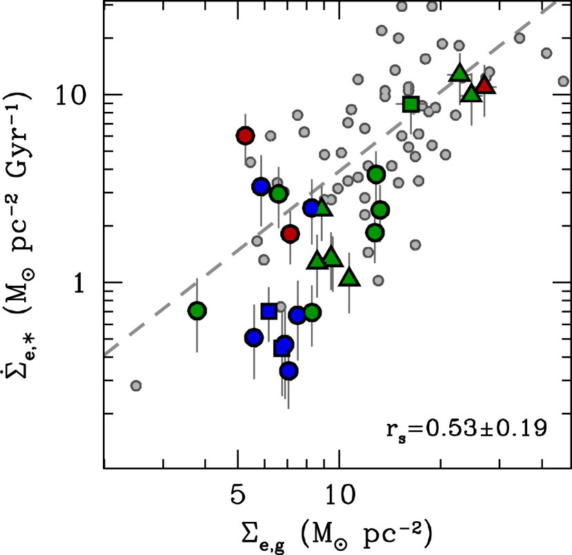
Figure 1.— Relation between $\dot{\Sigma}_{e,\ast}$ and $\Sigma_{e,g}$ for 25 galaxies from the DiskMass Survey. Green points are “bc” and “c” type spirals, with red and blue points being earlier and later types, respectively. Circles, triangles, and squares are unbarred (S), weakly barred (SAB), and barred (SB) galaxies, respectively. We provide the rank correlation coefficient, $r_{s}$, for our sample in the bottom-right corner. Gray points are the “Normal Spirals” from K98 and the gray dashed line is the nominal KS law. Both the data and fit from K98 have been offset to account for the factor of 1.4 we use to obtain the total gas mass.

3.3. Comparison with K98

We compare our sample to the “Normal Spirals” presented by K98 in Figure 1, where we have accounted for the factor of 1.4 difference between our calculation of $\Sigma_{e,g}$ and the hydrogen-only surface densities calculated by K98. Our galaxies are roughly consistent with the scatter seen in the K98 sample. Additionally, those galaxies with $\dot{\Sigma}_{e,\ast}<1\mathcal{M}_{\odot}$ pc^-2 Gyr^-1 (approximately one-third of our sample) are consistent with the well-known drop in $\dot{\Sigma}_{e,\ast}$ with respect to the nominal KS law at low $\Sigma_{e,g}$ (e.g., Bigiel et al., 2008, Figure 15). Most important to this comparison, our galaxy sample shows that $\dot{\Sigma}_{e,\ast}$ and $\Sigma_{e,g}$ are correlated.

We characterize the correlation between two quantities using the Spearman rank-order correlation coefficient ($r_{s}$, see Section 14.6.1 of Press et al., 2007). Exact (anti-)correlation yields $r_{s}=(-)1$. By using ranks, $r_{s}$ is independent of whether or not one considers the logarithmic or linear distribution of the data. Additionally, $r_{s}$ benefits over the linear (or Pearson) correlation coefficient because each datum (rank) is drawn from a known probability distribution, leading to a more straight-forward interpretation of the significance of the correlation as quantified via the $p$-value (Press et al., 2007). We estimate the error in the correlation coefficient using $10^{3}$ bootstrap simulations. The value of $r_{s}$ for our $\dot{\Sigma}_{e,\ast}$ and $\Sigma_{e,g}$ measurements is provided in Figure 1.

Although the correlation coefficient measured between $\Sigma_{e,g}$ and $\dot{\Sigma}_{e,\ast}$ is rather significant for our data (the $p$-value rejects the null hypothesis — no correlation — at better than 99% confidence), the robustness of the measurement is rather low (with $r_{s}$ being less than three times its error). The sample of “Normal Spirals” from K98 exhibit a much stronger correlation, both in terms of significance and robustness, with $r_{s}=0.66\pm 0.07$; however, the calculated $r_{s}$ for the two samples are consistent within the errors. If we fit a Schmidt relation to our data, we find a power-law slope that is within the error of the KS law, but we find a significantly different normalization. This can be attributed to the fact that approximately 80% of the galaxies in our sample fall below the nominal KS law. Throughout this paper, we therefore prefer to discuss the correlation between two quantities, as opposed to fitting regressions. We work under the assumption that the correlations we measure should be within the error of those found for larger samples. We will fit parameterized forms to our data — incorporating independent errors along both axes using Fitexy from Section 15.3 from Press et al. (2007) — when useful for comparing our data with a previous result or prediction from the literature, but these results are provided primarily for illustration purposes.

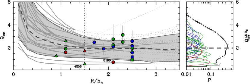
Figure 2.— Left — The multi-component disk stability parameter, $Q_{\rm RW}$, as a function of $R/h_{R}$, determined by the median of the posterior from our dynamical model of each galaxy. Regions directly constrained by $\sigma_{\ast}$ are shown as solid gray lines, whereas regions beyond this (dotted gray lines) are either constrained by the rotation curves or extrapolations of the model. The minimum value between $0.1\leq R/h_{R}\leq 2.5$, $Q_{\rm RW}^{\rm min}$, is marked for each galaxy; we have labeled the results for UGC 4256 and 8196. Colors and symbol types are the same as in Figure 1. The gray dashed line is the median of the marginalized distributions of $Q_{\rm RW}$ versus $R/h_{R}$ and the light-gray region shows the 68% confidence interval. The vertical dotted black line marks $R=1.5h_{R}$. Right — The probability distribution of $Q_{\rm RW}$ at 1.5 $h_{R}$ for each galaxy, color coded by Hubble type as in Figure 1. The black histogram is the probability distribution of $Q_{\rm RW}$ marginalized over all galaxies, with the integral normalized to unity; the gray dashed line is the median of this distribution. All other probability distributions have been normalized relative to their contribution to the total marginalized probability.

3.4. Stability Results

We calculate $Q_{\rm RW}$ as a function of radius (in units of the scale length, $h_{R}$) for 25 of the 27 galaxies in our sample as shown in Figure 2. The median radial profile of $Q_{\rm RW}$ marginalized over all galaxies is high near the center (largely driven by the epicyclic frequency) and asymptotes to a nearly constant value beyond $\sim$1 $h_{R}$.

Two galaxies — UGC 4256 and UGC 8196 — exhibit $Q_{\rm RW}<1$ over the majority of their disks, which is difficult to interpret. Either the dynamical assumptions made by our modeling approach have led to a value of $Q_{\rm RW}$ that is systematically in error or the disks of these two galaxies are, in actuality, unstable according to the criterion derived by Romeo & Wiegert (2011). In the case of UGC 4256, it might be reasonable to expect the latter because it has a rather massive molecular component (as measured by its 24$\mu$m surface brightness) relative to its stellar disk (Paper VII). Also, UGC 4256 likely suffered a recent interaction and it exhibits a one-armed, asymmetric morphology. However, these latter two observations contradict the assumptions made by our dynamical model, such that we might expect that the low $Q_{\rm RW}$ values are systematically in error. In the case of UGC 8196, the galaxy is bulge-dominated and an outlier in our maximality analysis with an overly massive baryonic disk; see Bershady et al. (2011, hereafter Paper V) and additional discussion of this galaxy in Paper VII. We continue to consider the results for these two galaxies below, but advise the reader to keep these caveats in mind.

For the remainder of the paper, we focus on two fiducial measurements of the stability level. First, we determine the minimum over the range $0.1\leq R/h_{R}\leq 2.5$, $Q_{\rm RW}^{\rm min}$. For 12 galaxies, the value of $Q_{\rm RW}^{\rm min}$ is taken at $2.5h_{R}$ because $Q_{\rm RW}$ continues to decrease beyond this radius such that the true minimum of $Q_{\rm RW}$ is not well constrained by the data. The determined values of $Q_{\rm RW}^{\rm min}$ are shown in Figure 2 and provided in Table 1. Second, we calculate $Q_{\rm RW}$ at 1.5 scale lengths, $Q_{\rm RW}^{1.5h_{R}}$, which is expected to be an optimal disk value, well away from any bulge component and often within the radial regime of our stellar velocity dispersion measurements. The conclusions we reach in Section 4 are very similar when considering either $Q_{\rm RW}^{\rm min}$ or $Q_{\rm RW}^{1.5h_{R}}$; however, the correlations with $Q_{\rm RW}^{\rm min}$ are strongest. Additionally, we are motivated to use $Q_{\rm RW}^{\rm min}$ such that we can more directly compare our measurements to the theoretical results from Li et al. (2006).

At $R=1.5h_{R}$, we find a full range of $0.6<Q_{\rm RW}^{1.5h_{R}}<3.4$ and a marginalized median of $2.0\pm 0.9$. This value for the disk stability parameter is close to the values often found in N-body simulations of galaxy disks (e.g., Roškar et al., 2012). However, we emphasize that this is a two-component stability level with corrections for disk thickness, whereas the majority of N-body simulations consider only the collisionless, single-component criterion from Toomre (1964). The stability parameter in equation 1 can be corrected such that it is valid for a single-component collisionless stellar system by calculating $\mathcal{Q}_{\ast}=\pi Q_{\ast}/3.36$ (Toomre, 1964). At 1.5$h_{R}$, we find marginalized median values of $Q_{g}=2.0^{+1.1}_{-0.7}$ and $\mathcal{Q}_{\ast}=2.9^{+5.0}_{-1.8}$ with ranges of $0.5\leq Q_{g}\leq 4.7$ and $0.5\leq\mathcal{Q}_{\ast}\leq 25$. We also find that $Q_{g}<\mathcal{Q}_{\ast}$ for approximately 65% of our sample, such that the calculation of $Q_{\rm RW}^{1.5h_{R}}$ is often dominated by the contribution of the gaseous component.

Our marginalized median value of $\langle Q_{\rm RW}^{1.5h_{R}}\rangle=2.0\pm 0.9$ agrees well with other empirical assessments. In particular, Romeo & Falstad (2013, see their Figure 5) studied the stability parameter in the galaxy sample presented by Leroy et al. (2008) and found a median value of $Q_{\rm RW}\sim 2$ over most of the optical radius. However, they also concluded that it is the stellar component that typically dominates the calculation of the two-component $Q_{\rm RW}$, whereas we find that it is the gas component that most often dominates. It is more likely that this difference is due to our different analysis methods rather than an intrinsic difference in the galaxy samples.

In terms of Hubble type, our galaxies range from Sa to Im (Table 1) and the Leroy et al. (2008) sample has a comparable range from Sab to Im type. However, our galaxies are more strongly concentrated toward Sc and Scd types, whereas the Leroy et al. (2008) is evenly distributed between Sb and Sd with a peak at Im types.

With respect to the stability level of the stellar component, Romeo & Falstad (2013) adopted the stellar mass surface densities and velocity dispersions calculated by Leroy et al. (2008). Leroy et al. assumed a $K$-band mass-to-light ratio of $\Upsilon_{K}=0.50\ \mathcal{M}_{\odot}/{L}_{\odot}^{K}$, an oblateness relation of $h_{R}/h_{z}=7.3$, and an isothermal disk ($k=2.0$) to calculate $\sigma_{R}$ using the adopted stellar surface density and $\alpha=0.6$. The most significant difference with respect to our approach is that, as shown in Section 3.4 of Paper VII, our dynamical calculations of the surface mass density yield a mean value of $\langle\Upsilon_{K}\rangle=0.31\ \mathcal{M}_{\odot}/{L}_{\odot}^{K}$. In total, we expect the approach of Romeo & Falstad (2013) leads to values of $\mathcal{Q}_{\ast}$ that are, on average, a factor of 0.8 times our own.

A more significant difference is in the calculation of $Q_{g}$. Our analysis assumes $\Sigma_{g}=1.4\Sigma_{H}$, $\sigma_{cg}=\sigma_{ig}/2$ (leading to a mean value of 8.3 km s^-1), and $X_{\rm CO}=2.7\times 10^{20}$ cm^-2 (K km s^-1)^-1; however, Leroy et al. (2008) adopt $\Sigma_{g}=\Sigma_{H}$, $\sigma_{cg}=11$ km s^-1, and $X_{\rm CO}=2.0\times 10^{20}$ cm^-2 (K km s^-1)^-1. The differences between our calculation and that from Romeo & Falstad (2013) are at their extrema when one assumes the gas is either fully atomic or fully molecular, such that their calculations of $Q_{g}$ should be, on average, factors of 1.9–2.5 times our own. This is likely why we find more galaxies with $Q_{g}<\mathcal{Q}_{\ast}$ than in the two-component analysis from Romeo & Falstad (2013, see also ).

We are confident in our calculations of $\mathcal{Q}_{\ast}$ due to our reliance on stellar kinematic data, as opposed to an inferred $\Upsilon_{K}$; yet our calculations of $Q_{g}$ (as well as those produced by Romeo & Falstad, 2013) do, unfortunately, depend on assumed factors. All of our assumptions are justified; however, our analysis would benefit from more direct constraints on the gas-phase metallicity, $\sigma_{cg}$, and $X_{\rm CO}$ for each galaxy.

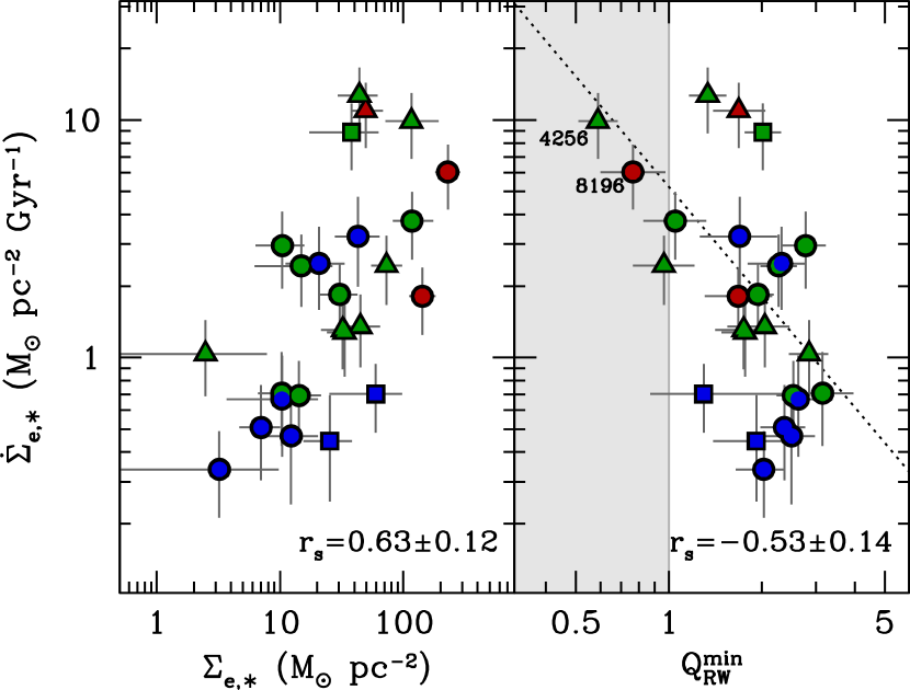
Figure 3.— The effective star-formation-rate surface density, $\dot{\Sigma}_{e,\ast}$, as a function of effective stellar mass surface density, $\Sigma_{e,\ast}$, and the minimum disk stability parameter, $Q_{\rm RW}^{\rm min}$. Colors and symbol types are the same as in Figure 1. The light-gray region denotes nominal disk instability. We provide $r_{s}$ in the bottom-right corner of each panel. The two galaxies with $Q_{\rm RW}<1$ over the majority of their disks (see Figure 2) are labeled in the right panel. The dotted line is the best fitting power-law relationship with a fixed power-law slope of -1.54 (Li et al., 2006). Our data appear to show a much steeper relationship (with a power-law slope of approximately -3).

4. (Anti-)Correlations with Star-Formation Rate

In this section, we explore correlations between $\dot{\Sigma}_{e,\ast}$, $\Sigma_{e,\ast}$, and $Q_{\rm RW}^{\rm min}$. We are the first to explore these correlations using measurements of stellar mass surface density and disk stability levels that are directly constrained by stellar kinematics.

Figure 3 demonstrates that our data show significant and robust correlations of $\Sigma_{e,\ast}$ and $Q_{\rm RW}^{\rm min}$ with $\dot{\Sigma}_{e,\ast}$; however, both panels in Figure 3 exhibit large scatter, with a range of up to 1.5 dex seen in $\dot{\Sigma}_{e,\ast}$ at fixed $\Sigma_{e,\ast}$ or fixed $Q_{\rm RW}^{\rm min}$. By comparison, this range is reduced to approximately 1 dex when considering $\dot{\Sigma}_{e,\ast}/\Sigma_{e,g}$ (the SFE, see Figure 4) instead. Nonetheless, the correlation between $\Sigma_{e,\ast}$ and $\dot{\Sigma}_{e,\ast}$ shown in Figure 3 is the strongest and most robust of those presented in this paper. We find $\dot{\Sigma}_{e,\ast}$ is anti-correlated with $Q_{\rm RW}^{\rm min}$ at better than 99% confidence considering both the null hypothesis and the error in $r_{s}$; however, neither gas-only nor star-only stability calculations exhibit such a correlation. Thus, we find that in relating disk stability levels to star formation, it is important to incorporate both components, gas and stars, in the stability assessment.

Based on GADGET N-body simulations of gaseous disk galaxies (using smoothed particle hydrodynamics), Li et al. (2006) find $\dot{\Sigma}_{\ast}\propto[Q_{sg,{\rm min}}(\tau_{\rm SF})]^{-1.54}$. In their analysis, they adopt the stability parameter derived by Rafikov (2001), using the wavenumber of the perturbation that yields the minimum two-component (gas$+$stars) disk stability level, and they refer to this as $Q_{sg}$. Romeo & Falstad (2013) have shown that $Q_{\rm RW}$ is a good approximation to this usage of the Rafikov (2001) formulation, but without the need to determine the minimizing wavenumber. The value $Q_{sg,{\rm min}}(\tau_{\rm SF})$ provided by Li et al. (2006) is the minimum value of $Q_{sg}$ over all radii at one $e$-folding time of the star-formation rate, $\tau_{\rm SF}$. Under the expectation that our galaxies are all quiescently star-forming and that the evolution of $Q_{sg}$ is moderate at $t>\tau_{\rm SF}$, the above proportionality from Li et al. (2006) should be reflected in Figure 3. A caveat to this comparison is that the galaxy simulations in Li et al. (2006) were of largely unstable disks with $Q_{sg,{\rm min}}(\tau_{\rm SF})\lesssim 1$.

The dotted line in Figure 3 is a fit to our data done by fixing the slope to that expected by Li et al. (2006). Our data appear to follow a much steeper relation, with a power-law slope that is approximately -3. However, we note that the correlation seen between $Q_{\rm RW}^{\rm min}$ and $\dot{\Sigma}_{e,\ast}$ depends rather strongly on the two galaxies with $Q_{\rm RW}<1$ over most of the disk.

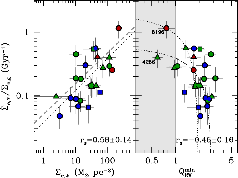
Figure 4.— The star-formation efficiency (SFE), $\dot{\Sigma}_{e,\ast}/\Sigma_{e,g}$, as a function of effective stellar mass surface density, $\Sigma_{e,\ast}$, and minimum disk stability parameter, $Q_{\rm RW}^{\rm min}$. Colors, symbol types, and the light-gray region are the same as in Figure 3. In the left panel, the dotted line is the best-fitting power law with a power-law slope of 0.5, showing consistency with the expectation of OML10; the gray dashed line is the relation from Shi et al. (2011). In the right panel, the dotted line shows the best-fitting linear relationship with a slope of -1.0 (Li et al., 2006), whereas the dot-dashed line shows the best fit when both the slope and intercept are free parameters. Both panels exhibit a correlation; however, the correlation between $Q_{\rm RW}^{\rm min}$ and the SFE is rather weak.

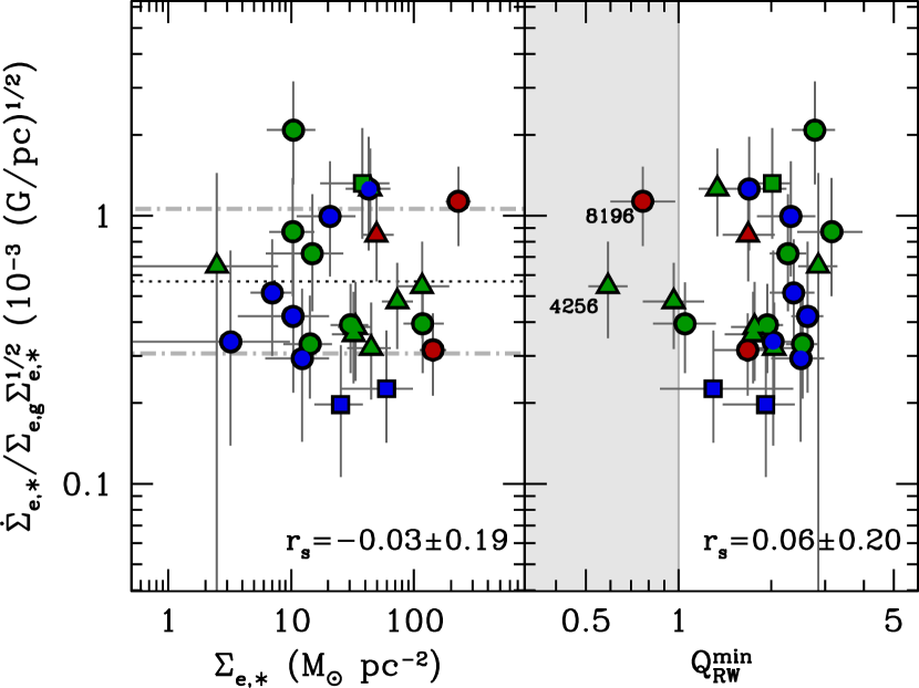
Figure 5.— The expected constant of proportionality for $\dot{\Sigma}_{e,\ast}/\Sigma_{e,g}\propto\Sigma_{e,\ast}^{1/2}$ as a function of effective stellar mass surface density, $\Sigma_{e,\ast}$, and minimum disk stability parameter, $Q_{\rm RW}^{\rm min}$. Colors, symbol types, and the light-gray region are the same as in Figure 3. The dotted line and the gray dot-dashed lines in the left panels gives the error-weighted geometric mean and standard deviation, respectively: $\langle\log(\dot{\Sigma}_{e,\ast}\Sigma_{e,g}^{-1}\Sigma_{e,\ast}^{-1/2})\rangle=-3.25\pm 0.27$ in units of $(G/{\rm pc})^{1/2}$.

Li et al. (2006) also predict a linear relationship between $\dot{\Sigma}_{e,\ast}/\Sigma_{e,g}$ and $Q_{\rm RW}^{\rm min}$. Leroy et al. (2008) found no evidence for such a correlation using spatially resolved observations. However, Figure 4 shows that our data exhibit a weak correlation between $\dot{\Sigma}_{e,\ast}/\Sigma_{e,g}$ and $Q_{\rm RW}^{\rm min}$, which is again highly dependent on the two galaxies with $Q_{\rm RW}^{\rm min}<1$. Figure 4 shows the best-fitting linear relationship with a slope of -1.0 (dotted line; as expected by Li et al., 2006) and the result after fitting both the slope and intercept (we find a best-fitting slope of -0.2; dot-dashed line). Thus, our data are at least suggestive of the relation expected by Li et al. (2006), albeit qualitatively.

Figure 4 also shows the correlation of $\dot{\Sigma}_{e,\ast}/\Sigma_{e,g}$ with $\Sigma_{e,\ast}$. Our data are consistent with the empirical result from Shi et al. (2011), and with a proportionality derived by OML10 for the outer parts of stellar-dominated, constant-scale-height disks, $\dot{\Sigma}_{e,\ast}/\Sigma_{e,g}\propto\Sigma_{e,\ast}^{1/2}$. The dotted line in the left panels of Figures 4 and 5 show the result of fitting this proportionality to our data. Given the order of magnitude range in $\dot{\Sigma}_{e,\ast}\Sigma_{e,g}^{-1}\Sigma_{e,\ast}^{-1/2}$, we might expect other correlations to exist. However, we find no residual correlations of this quantity with respect to, e.g., $h_{z}$, $v_{c}$, $\kappa$, $\sigma_{R}$, $\sigma_{cg}$, $\alpha$, $\Sigma_{e,g}$, $\Sigma_{e,\ast}$, $\Sigma_{e,g}/\Sigma_{e,\ast}$, or $Q_{\rm RW}^{\rm min}$ (Figure 5): the significance of all correlations are low with $|r_{s}|<0.2$ and the measurements of $r_{s}$ are all consistent with no correlation according to their error. In units of $(G/{\rm pc})^{1/2}$, we find an error-weighted geometric mean of $\langle\log(\dot{\Sigma}_{e,\ast}\Sigma_{e,g}^{-1}\Sigma_{e,\ast}^{-1/2})\rangle=-3.25\pm 0.27$. This result is further discussed in Section 6.

5. An Expectation from Scaling Relations

Instead of exploring a theoretical understanding of the correlation between $\dot{\Sigma}_{e,\ast}$ and $Q_{\rm RW}$ shown in Section 4, we ask two questions. Given other (selected) ensemble properties of late-type galaxies, should we expect an anti-correlation between $\dot{\Sigma}_{e,\ast}$ and $Q_{\rm RW}$? If so, does that expectation match our direct measurements? We address these questions by building a closed system of empirical scaling relations (i.e., the number of equations matches the number of unknowns) from which we can compute $Q_{\rm RW}$ for a given $\dot{\Sigma}_{\ast}$ in an idealized galaxy.

5.1. Calculation Details

Equations 1, 2, and 5–7 require $v_{c}$, $\sigma_{cg}$, $\sigma_{R}$, $\Sigma_{g}$, and $\Sigma_{\ast}$ to produce $Q_{\rm RW}$. For the calculation, we ignore the effects of any bulge component and assume a constant $K$-band mass-to-light ratio, $\Upsilon_{K}$ (cf. Paper VII, ). We assume $\sigma_{cg}$ is constant and we set it directly. The remaining four quantities are determined by setting $\dot{\mathcal{M}}_{\ast}$, the disk central surface brightness ($\mu_{0,K}$), $h_{R}$, $R_{25}$, $\Upsilon_{K}$, and $\alpha$ and combining these quantities with a set of empirical scaling relations as described below. We emphasize that we are not suggesting that our seven input parameters are the fundamentally relevant physical quantities of a galaxy (in the same sense as mass, age, and chemical composition are relevant to a star); these are simply the quantities that we need to calculate $Q_{\rm RW}$.

The input parameters set $\Sigma_{\ast}(R)=\Sigma_{\ast,0}\exp(-R/h_{R})$ directly, where $\Sigma_{\ast,0}=\Upsilon_{K}I_{0,K}$, $\log I_{0,K}=-0.4(\mu_{0,K}-M_{\odot,K}-21.57)$, and $M_{\odot,K}=3.3$ is the absolute $K$-band magnitude of the sun (Paper IV); $\Upsilon_{K}$ is in solar units ($\mathcal{M}_{\odot}/{L}_{\odot}^{K}$) and $I_{0,K}$ is in units of ${L}_{\odot}^{K}~{}\!$pc^-2. We calculate $\sigma_{R}(R)=\sigma_{z}(R)/\alpha$ using the input value of $\alpha$ and

$$\sigma_{z}=(\pi\ k\ G\ h_{z}\ \Sigma_{\rm dyn})^{1/2},$$ (9)

where $\Sigma_{\rm dyn}=\Sigma_{\ast}+\Sigma_{g}$ and $k=1.5$ for an exponential mass distribution (van der Kruit, 1988); we determine $h_{z}$ using its scaling with $h_{R}$ from Paper II.

We parameterize the circular-speed curve by a hyperbolic tangent function that has two parameters: the asymptotic rotation speed ($V_{\rm rot}$) and the radius ($h_{\rm rot}$) at which $v_{c}=\tanh(1.0)V_{\rm rot}=0.76V_{\rm rot}$. We have chosen this form so that we can set its parameters based on two scaling relations. First, Andersen & Bershady (2013, Figure 17) find

$$\log h_{\rm rot}=\log h_{R}-0.714\log\left[\frac{V_{\rm rot}}{\mbox{{km$~{}\!$s${}^{-1}$}}}\right]+1.47,$$ (10)

which is in good agreement with the scaling relation found by Amorisco & Bertin (2010) but adds a secondary dependence on the rotation velocity. Second, we use the relation between disk maximality ($\mathcal{F}^{2.2}_{\rm bary}=V_{\rm bary}/V_{c}$ at $R=2.2h_{R}$) and $\mu_{0,K}$ from Paper VII: $\mathcal{F}^{2.2}_{\rm bary}=0.56-0.08(\mu_{0,K}-18)$. We calculate the baryonic disk rotation speed,

$$V_{\rm bary}=0.88\left(1-0.28\frac{h_{R}}{h_{z}}\right)(\pi G\Sigma_{{\rm dyn},0}h_{R})^{2},$$ (11)

following Paper V. Equation 11 assumes that $\Sigma_{\rm dyn}$ follows a pure exponential with a scale length equal to that of the stars. However, this is only explicitly true in the limit where there is no gas disk. For our calculations, we adopt the rough approximation

$$\Sigma_{{\rm dyn},0}=\Sigma_{g,R}\exp(R/h_{R})+\Sigma_{\ast,0},$$ (12)

where $\Sigma_{g,R}$ is the gas mass surface density at radius $R$ (see below). We numerically solve for $V_{\rm rot}$ and $h_{\rm rot}$ given the input $\mu_{0,K}$, $\Upsilon_{K}$, and $h_{R}$, and the calculated $\Sigma_{{\rm dyn},0}$.

We use two approaches to define the functional form of $\Sigma_{g}(R)$, which is then normalized by the star-formation law (see below). First, Bigiel & Blitz (2012) found the total hydrogen mass is well described by a single exponential with an $e$-folding length of $0.61R_{25}$. We term this the “BB” approach. Second, we separate the hydrogen mass into its molecular and atomic components according to the scaling relation found by Saintonge et al. (2011):

$$\log\left[\frac{\mathcal{M}_{\mbox{\rm\footnotesize H{i}}}}{\mathcal{M}_{\odot}}\right]=1.01\left(\log\left[\frac{\mathcal{M}_{\mbox{\footnotesize H${}_{2}$}}}{\mathcal{M}_{\odot}}\right]+0.42-\log\left[\frac{X_{\rm CO}}{2.0}\right]\right),$$ (13)

where $\mathcal{M}_{\mbox{\rm\footnotesize H{i}}}+\mathcal{M}_{\mbox{\footnotesize H${}_{2}$}}$ is the total hydrogen mass and we have generalized the relation for any (constant) $X_{\rm CO}$ in units of $10^{20}$ cm^-2 (K km s^-1)^-1; Paper VII shows equation 13 is fully consistent with our galaxy sample. We assume $\Sigma_{\rm H_{2}}$ follows an exponential with the same scale length as the stars (Regan et al., 2001), and $\Sigma_{\mbox{\rm\footnotesize H{i}}}$ follows a Gaussian in radius with a center and dispersion of, respectively, $0.39R_{\mbox{\rm\footnotesize H{i}}}$ and $0.35R_{\mbox{\rm\footnotesize H{i}}}$ (Martinsson, 2011). We calculate $R_{\mbox{\rm\footnotesize H{i}}}$ — the radius at which $\Sigma_{\mbox{\rm\footnotesize H{i}}}\sim 1$ $\mathcal{M}_{\odot}~{}\!$pc^-2— using the relation derived by Verheijen & Sancisi (2001):

$$\log\left[\frac{R_{\mbox{\rm\footnotesize H{i}}}}{\rm kpc}\right]=(\log\left[\frac{\mathcal{M}_{\mbox{\rm\footnotesize H{i}}}}{\mathcal{M}_{\odot}}\right]-7.26)/1.86.$$ (14)

Finally, we use Brent’s minimization method (Press et al., 2007) to solve the set of non-linear equations that yield the defining parameters for $\Sigma_{\mbox{\rm\footnotesize H{i}}}(R)$ and $\Sigma_{\rm H_{2}}(R)$. We term this the “MA” approach. In both approaches, we set $\Sigma_{g}=1.4\Sigma_{\rm H}=1.4(\Sigma_{\mbox{\rm\footnotesize H{i}}}+\Sigma_{\rm H_{2}})$.

Finally, we use two star-formation laws to determine the normalization of the hydrogen mass surface density profile. First, we adopt the KS law from K98:

$$\log\left[\frac{\Sigma_{\rm e,H}}{\mathcal{M}_{\odot}{\rm pc}^{-2}}\right]=0.71\ \log\left[\frac{\dot{\Sigma}_{e,\ast}}{\mathcal{M}_{\odot}{\rm pc}^{-2}{\rm Gyr}^{-1}}\right]+0.47,$$ (15)

where $\Sigma_{\rm e,H}$ is the effective hydrogen mass surface density within $R_{25}$ and we calculate $\dot{\Sigma}_{e,\ast}=\dot{\mathcal{M}}_{\ast}/\pi R_{25}^{2}$, as done for our data. Second, we assume

$$\log\left[\frac{\Sigma_{\rm e,H}}{\mathcal{M}_{\odot}{\rm pc}^{-2}}\right] = \log\left[\frac{\dot{\Sigma}_{e,\ast}}{\mathcal{M}_{\odot}{\rm pc}^{-2}{\rm Gyr}^{-1}}\right]+1.15$$ (16)

$$-0.48\log\left[\frac{\Sigma_{e,\ast}}{\mathcal{M}_{\odot}{\rm pc}^{-2}}\right]$$

from Shi et al. (2011, see their Equation 6), where we have adjusted for their factor of 1.36 used to obtain the total gas mass surface density from the hydrogen mass surface density. We follow their nomenclature by referring to this as the “extended Schmidt” (ES) law. The combinatorics of the two star-formation laws and the two approaches used to distribute the hydrogen mass lead to four methods for calculating $Q_{\rm RW}$.

Table 2 $\delta Q$ Quartiles

	Approach
Growth	KS:MA	KS:BB	ES:MA	ES:BB
0.25	0.12	0.12	0.18	0.14
0.50	0.21	0.24	0.23	0.23
0.75	0.44	0.38	0.45	0.47
1.00	0.72	0.55	1.55	0.70

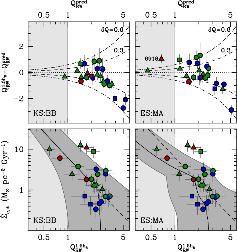
Figure 6.— Comparison of predicted $Q_{\rm RW}$ with the measured values at $1.5h_{R}$; panels to the left and right use the KS:BB and ES:MA approaches, respectively. Colors, symbol types, and the light-gray region are the same as in Figure 3. The top panels show the difference between the measured $Q_{\rm RW}^{1.5h_{R}}$ and the prediction. The dashed and dot-dashed lines show a ratio of the two axes equal to $\pm 0.3$ and $\pm 0.6$, respectively. The bottom panels show the measurements of $\dot{\Sigma}_{e,\ast}$ and $Q_{\rm RW}^{1.5h_{R}}$. The solid black line in each panel predicts the correlation between these two quantities assuming the mean properties of our galaxy sample; the black dashed line, shown in both panels, is a power-law fit to the KS:BB result between $0.5<Q_{\rm RW}^{\rm pred}<2.0$. The dark-gray region is the envelope encompassing all correlations generated when using the values of $\Upsilon_{K}$, $\mu_{0,K}$, $h_{R}$, $R_{25}$, $\alpha$, and $\sigma_{cg}$ specific to each galaxy.

5.2. Results

We first compare our measurements of $Q_{\rm RW}$ from the modeling of our data to the predictions based on the calculations described above. Any difference can be directly attributed to the systematic errors in our simplifying assumptions; e.g., the assumption for the detailed form of the surface density profiles. To focus the following discussion, we compare the data, $Q_{\rm RW}^{1.5h_{R}}$, and the prediction, $Q_{\rm RW}^{\rm pred}$, at a single radius, 1.5$h_{R}$, and define the quantity $\delta Q=\left|Q_{\rm RW}^{1.5h_{R}}/Q_{\rm RW}^{\rm pred}-1\right|$. Our comparison of the data with the model at 1.5$h_{R}$ is unimportant to our conclusions because both the model and the data (Figure 2) exhibit a slow change in $Q_{\rm RW}$ beyond this radius.

We provide quartiles of $\delta Q$ in Table 2, the left-most column gives the growth of $\delta Q$ and the remaining columns give its value for the four different approaches to the calculation. The predicted disk stability parameters are within 25% of the measured values for half of our galaxy sample, regardless of the approach used. For the entire sample however, Table 2 shows the KS:BB and ES:MA methods are, respectively, the best and worst approaches for predicting $Q_{\rm RW}$. Interestingly, KS:BB is the simplest approach and ES:MA is the most complex. We continue by only comparing these two approaches and discussing their predictions.

The top two panels of Figure 6 show the individual results in the comparison of $Q_{\rm RW}^{1.5h_{R}}$ and $Q_{\rm RW}^{\rm pred}$. Lines are provided that denote $\delta Q=0.0$, 0.3, and 0.6. Thus, we show that the maximum value for $\delta Q$ when using the ES:MA method is largely due to the outlying prediction for UGC 6918 (labeled in the top-right panel of Figure 6). We also find three late-type spirals that have a rather large $Q_{\rm RW}^{\rm pred}$ for the KS:BB method; this is likely due to their significantly larger value of $\Sigma_{e,g}$ than that predicted by the KS law (see Figure 1). Despite these caveats, our prediction of $Q_{\rm RW}^{1.5h_{R}}$ is reasonable in either approach with $\delta Q\approx 0.35$ at 68% growth.

The bottom two panels of Figure 6 compare the measured and predicted trend of $Q_{\rm RW}$ with $\dot{\Sigma}_{e,\ast}$. Our combination of empirical scaling relations predict an anti-correlation between $\dot{\Sigma}_{e,\ast}$ and $Q_{\rm RW}$: Adopting the (unweighted) average properties of our sample — $\sigma_{cg}=8.3$ km s^-1, $\mu_{0,K}=17.8$ mag arcsec^-2, $h_{R}=4.3$ kpc, $R_{25}=18.0$ kpc, $\Upsilon_{K}=0.36\mathcal{M}_{\odot}/{L}_{\odot}^{K}$, and $\alpha=0.57$ — we vary $\dot{\mathcal{M}}_{\ast}$ to produce the black line in each of the bottom panels of Figure 6. However, the behavior of the two methods is different.

Both methods exhibit an inflection in the trend at $Q_{\rm RW}^{\rm pred}>2$, which occurs because the calculation of $Q_{\rm RW}$ transitions to the regime where $\mathcal{T}_{\ast}Q_{\ast}<\mathcal{T}_{g}Q_{g}$ at higher $Q_{\rm RW}^{1.5h_{R}}$ (see Equation 6). For $Q_{\rm RW}^{\rm pred}<2$, the KS:BB approach yields a well-behaved relationship between $\dot{\Sigma}_{e,\ast}$ and $Q_{\rm RW}^{\rm pred}$ due to its simple description of the gas distribution: a power-law slope of -2.07 is an excellent fit to the KS:BB results between $0.5<Q_{\rm RW}^{\rm pred}<2.0$ (as shown by the dashed line).

The behavior of the ES:MA method is more complex, exhibiting a second inflection of the trend at $Q_{\rm RW}^{\rm pred}<2$. This inflection occurs because, as $\dot{\Sigma}_{e,\ast}$ increases, the dependence of the H i distribution on its total mass results in a transition from an H i-dominated $\Sigma_{g}$ to an H₂-dominated $\Sigma_{g}$ at $1.5h_{R}$. The dependence of the H i distribution on its total mass in the MA approach significantly contributes to its larger $\delta Q$. The MA approach suggests two-thirds of the galaxies have $R_{\mbox{\rm\footnotesize H{i}}}/R_{25}<1$, whereas our direct measurements show $R_{\mbox{\rm\footnotesize H{i}}}/R_{25}>1$ for all galaxies (Martinsson, 2011). This failing is due to the low $\Sigma_{e,g}$ predicted by the ES and KS laws at low $\dot{\Sigma}_{e,\ast}$, not due to our adoption of equation 14. The $\mathcal{M}_{\mbox{\rm\footnotesize H{i}}}$-$R_{\mbox{\rm\footnotesize H{i}}}$ relation is very tight such that, when considered as an isolated sample, our galaxies exhibit a very similar scaling relation (Martinsson, 2011).

Instead of adopting the mean properties of our sample, we have also calculated the trend of $Q_{\rm RW}^{\rm pred}$ with $\dot{\Sigma}_{e,\ast}$ when adopting the specific properties of each galaxy. We represent the range in the resulting trends using the dark-gray envelope about the black line in the lower two panels of Figure 6. Galaxies should populate this region in so far as our galaxy sample is representative of the range of $\Upsilon_{K}$, $\mu_{0,K}$, $h_{R}$, $R_{25}$, $\alpha$, and $\sigma_{cg}$ for late-type galaxies (Paper I) and considering the systematic errors in $Q_{\rm RW}^{\rm pred}$. Therefore, our results show that one should expect a correlation between $Q_{\rm RW}$ and $\dot{\Sigma}_{e,\ast}$ in a galaxy population, particularly at $Q_{\rm RW}^{1.5h_{R}}<2$.

6. Summary & Discussion

6.1. Summary of Analyses and Empirical Findings

In this paper, we have used data from the DiskMass Survey, briefly described in Section 2, to study the relationship between dynamical properties of galaxy disks and their star-formation activity. Unlike other local-universe surveys, the DiskMass Survey has directly measured the stellar kinematics in a sample of galaxy disks, which are critical to dynamical calculations of both stellar surface mass density and disk stability level. Our calculations are based on a generative — fully probabilistic — model of the relevant gaseous and stellar observations, adopting a simple analytical model for the disk dynamics. We introduce our probabilistic modeling approach in Section 3.1, we briefly outline the dynamical model in Appendix A, and we discuss our usage of a sophisticated MCMC algorithm to sample the probabilistic model in Appendix B. A more complete discussion of our modeling approach will be the subject of a forthcoming paper.

We calculate the star-formation rate, $\dot{\mathcal{M}}_{\ast}$, for each of our galaxies using measurements of the 21cm radio continuum (NVSS; Martinsson, 2011) and the calibrations from Yun et al. (2001) (see Section 3.2). These calculations are performed by including appropriate probability distributions for the relevant quantities in our probabilistic model (equation 4). We calculate an effective star-formation-rate surface density, $\Sigma_{\rm SFR}\equiv\dot{\Sigma}_{e,\ast}$, where the surface area of the disk is determined by $R_{25}$ measurements from NED (Table 1). Combined with effective gas mass surface densities from our probabilistic model (equation 8), we compare our galaxy sample to the “Normal Spirals” from K98 in Section 3.3 (see Figure 1). We find that the galaxies in our sample have low star-formation rates relative to the KS law, but are fully consistent with the low star-formation end of the data presented by Bigiel et al. (2008).

We calculate the disk stability parameter derived by Romeo & Wiegert (2011), $Q_{\rm RW}$, which incorporates both the gaseous and stellar components (see Section 3.2) and includes corrections for the disk thickness. In Section 3.4, we find a stability parameter of $Q_{\rm RW}=2.0\pm 0.9$ at 1.5 $h_{R}$ marginalized over all galaxies in our sample. This result is comparable to other empirical assessments from the literature. In particular Romeo & Falstad (2013) similarly find $Q_{\rm RW}\sim 2$ for their sample; however, they also find that the stellar component most often dominates the disk stability level. This is contrary to our results, which show that the gas-only stability parameter is lower than the star-only stability parameter ($Q_{g}<\mathcal{Q}_{\ast}$) for 65% of our sample. These different findings are more likely because of differences in the data used and the detailed analysis methods, as described in Section 3.4, not because of an intrinsic difference in our galaxy samples.

A stability parameter of $Q_{\rm RW}\sim 2$ is also comparable to expectations from N-body simulations; however, it should be noted that these theoretical studies typically calculate the nominal (infinitely thin, single-component, collisionless) Toomre (1964) criterion ($\mathcal{Q}_{\ast}$), as opposed to our calculations for a multi-component, non-zero thickness disk. An important avenue for numerical simulations of galaxy disks is to study the stability levels of disks that include realistic gas components.

The primary goal of this paper has been to explore any dependence of the star-formation rate on two dynamical properties of our sample, $\Sigma_{e,\ast}$ and $Q_{\rm RW}$ (see Section 4). Our primary findings are:

• There is a clear correlation between $\Sigma_{e,\ast}$ and $\dot{\Sigma}_{e,\ast}$ and a clear anti-correlation of $Q_{\rm RW}^{\rm min}$ with $\dot{\Sigma}_{e,\ast}$ (Figure 3).

• The anti-correlation between $Q_{\rm RW}^{\rm min}$ and $\dot{\Sigma}_{e,\ast}$ is expected given a theoretical study by Li et al. (2006). However, our galaxies exhibit significantly higher stability levels than in their simulations and our data show a steeper power-law slope in the relation.

• We find that the star-formation efficiency (SFE; $\dot{\Sigma}_{e,\ast}/\Sigma_{e,g}$) is correlated with $\Sigma_{e,\ast}$ (Figure 4), which is expected both observationally (Shi et al., 2011) and theoretically (OML10). In detail, our data are consistent with the proportionality $\dot{\Sigma}_{e,\ast}/\Sigma_{e,g}\propto\Sigma_{e,\ast}^{1/2}$, which is a limiting behavior of the theory derived by OML10; see also Kim et al. (2011, 2013).

• If star formation in our galaxy sample is not strongly affected by other physical properties, the quantity $\dot{\Sigma}_{e,\ast}\Sigma_{e,g}^{-1}\Sigma_{e,\ast}^{-1/2}$ should be roughly constant. Indeed, we find that this quantity is effectively uncorrelated with the large number of physical quantities we have calculated (listed in Section 4; see the examples of $\Sigma_{e,\ast}$ and $Q_{\rm RW}^{\rm min}$ in Figure 5). However, the scatter in the data is large. We find an error-weighted geometric mean of $\langle\log(\dot{\Sigma}_{e,\ast}\Sigma_{e,g}^{-1}\Sigma_{e,\ast}^{-1/2})\rangle=-3.25\pm 0.27$ in units of $(G/{\rm pc})^{1/2}$ and a range of $-3.7\leq\log(\dot{\Sigma}_{e,\ast}\Sigma_{e,g}^{-1}\Sigma_{e,\ast}^{-1/2})\leq-2.7$.

• Although the correlation is weak, we also find an indication that the SFE is anti-correlated with $Q_{\rm RW}^{\rm min}$ (Figure 4). This contradicts previous observational studies (Leroy et al., 2008), but is roughly consistent with the expectation provided by Li et al. (2006).

The anti-correlation between star-formation rate and disk stability parameter from Figure 3 is not seen if we instead consider the gas-only ($Q_{g}$) or star-only ($\mathcal{Q}_{\ast}$) stability parameters. In terms of the effect on star formation, this result is reasonable in that neither $Q_{g}$ nor $\mathcal{Q}_{\ast}$ includes the gravitational effects of the other component. Thus, our results show the importance of considering both components in assessing the effect of the disk stability level on star formation.

In Section 5, we quantitatively predict $Q_{\rm RW}$ at 1.5$h_{R}$ for the galaxies in our sample based on a closed system of scaling relations and the following global quantities for our galaxies: $\dot{\mathcal{M}}_{\ast}$, $\Upsilon_{K}$, $\mu_{0,K}$, $h_{R}$, $R_{25}$, $\sigma_{cg}$, and $\alpha=\sigma_{z}/\sigma_{R}$. The accuracy of the prediction depends on the details of the assumed mass distributions; however, all four approaches we discuss exhibit systematic errors of roughly 35% (68% confidence interval). Assuming our galaxy sample is representative of the overall population (Paper I), our calculations demonstrate that one should expect an anti-correlation between $\dot{\Sigma}_{e,\ast}$ and $Q_{\rm RW}$, particularly for $Q_{\rm RW}^{1.5h_{R}}<2$.

6.2. A Physical Link Between Disk Stability Level and Star Formation?

Our use of empirical scaling relations to predict the anti-correlation between $\dot{\Sigma}_{e,\ast}$ and $Q_{\rm RW}^{1.5h_{R}}$ suggests that this outcome is consistent with the physical drivers of other morphological and dynamical outcomes of late-type-galaxy evolution. However, does the anti-correlation imply a physical link between disk stability level and star formation?

The studies of Li et al. (2005, 2006) are particularly relevant because the star-formation in their simulations is, in fact, driven by gravitational instabilities, and our data are roughly consistent with their predictions (Figures 3 and 4). However, most of our galaxies are very stable, in the regime in which Li et al. (2005) find that it is difficult to form stars ($Q_{\rm RW}^{\rm min}\gtrsim 1.6$). A comparison of Figure 10 from Li et al. (2006) with our Figure 3 shows that our galaxies exhibit higher stability levels at the low star-forming end. Part of this discrepancy is due to systematic differences in our calculation of the stability parameter (e.g., our applied corrections for disk thickness); however, our data should yield relatively large stability values even after removing these systematic differences. Thus, just as seen via ultraviolet radiation in the very extended parts of disks (Thilker et al., 2007), our measurements suggest that star-formation occurs in locales with high stability levels. One theory that addresses this phenomenon is provided by OML10.

OML10 (see also Kim et al., 2011) present a model for star formation where the interstellar medium (ISM) is divided into self-gravitating and diffuse components. The pressure in the diffuse gas — regulated by heating, cooling, and supernova-driven turbulence — is assumed to be balanced by the vertical gravitational forces of the disk. A fundamental assumption is that the surface density of gravitationally bound clouds is converted to stars over a star-formation timescale; however, this timescale ($\sim$2 Gyr) is much longer than the free-fall time. The proportionality $\dot{\Sigma}_{\ast}/\Sigma_{g}\propto\Sigma_{\ast}^{1/2}$ is a limiting behavior of their model, assuming the star-formation rate in all galaxies is similarly affected by chemical composition, turbulence, and magnetic fields. We have shown in Figure 4 that this proportionality is consistent with our data, albeit with significant scatter. We have not assessed the variations in metallicity, turbulent pressure, or magnetic field strength in our sample, such that this may explain some of the scatter seen in our data.

The correspondence of our data with the limiting behavior of the OML10 prediction suggests that our galaxies form stars at a rate that maintains the pressure balance in the diffuse ISM. Such star formation does not require large-scale gravitational instabilities, but it does require the vertical gravitational field, largely effected by the stellar component in most cases, to maintain the total pressure in the disk midplane. Thus, star-formation can be active in the disks of our galaxies, despite our rather large measurements of $Q_{\rm RW}$. This may argue against a physical link between $Q_{\rm RW}$ and $\dot{\Sigma}_{e,\ast}$ at large $Q_{\rm RW}$.

However, the consistency of the trend seen in Figure 3 with the prediction of Li et al. (2006) at low $Q_{\rm RW}$ is suggestive of the role gravitational instabilities play in this small subset ($\sim$15%) of our sample. Therefore, a direct physical link between the stability level of galaxy disks and their star-formation activity may only be relevant to a small subset of the galaxies in the local universe; however, the story is most likely very different at earlier cosmic epochs (see, e.g., Agertz et al., 2009).

6.3. Spiral Structure Effects

A detailed analysis of the spiral-arm strength in our galaxy sample is beyond the scope of this paper; however, Figure 9 from Paper I shows that spiral arms are easily discernible in all of our sample galaxies. From N-body simulations, we expect spiral structure to be more easily generated in disks with lower $\mathcal{Q}_{\ast}$. If we assume that the same is true for $Q_{\rm RW}^{\rm min}$, we might expect effects related to spiral arms to be more evident in galaxies with lower $Q_{\rm RW}^{\rm min}$.

In their appendix, OML10 discuss the effects of spiral structure on their equilibrium model. They find that the azimuthally averaged (or disk-averaged) star-formation-rate surface density should be significantly lower than the true value if the contrast between the arm and inter-arm gas mass surface density is sufficiently high. If this effect were evident in our data, we may expect the residuals of our galaxy sample about $\dot{\Sigma}_{e,\ast}\Sigma_{e,g}^{-1}\Sigma_{e,\ast}^{-1/2}=10^{-3.25}$ $(G/{\rm pc})^{1/2}$ to be related to the strength of the spiral structure and therefore to $Q_{\rm RW}^{\rm min}$. However, Figure 5 shows no such relation. This may be because (1) $Q_{\rm RW}^{\rm min}$ is not a good proxy for the mass-loading of spiral-arm density waves, (2) our galaxies have all been similarly affected by spiral structure such that these properties have only changed the mean value of $\dot{\Sigma}_{e,\ast}\Sigma_{e,g}^{-1}\Sigma_{e,\ast}^{-1/2}$, (3) the timescales involved in the passage or lifetime of spiral arms is such that the equilibrium is never fully realized or substantially altered within the spiral-arm regions, or (4) the scatter in $\dot{\Sigma}_{e,\ast}\Sigma_{e,g}^{-1}\Sigma_{e,\ast}^{-1/2}$ caused by spiral arms or other physical processes has obscured the relation. Some of the scatter in our measurements of $\dot{\Sigma}_{e,\ast}\Sigma_{e,g}^{-1}\Sigma_{e,\ast}^{-1/2}$ can be attributed to systematic error; however, there is room for intrinsic scatter as well. It is of great interest to understand the scatter in $\dot{\Sigma}_{e,\ast}\Sigma_{e,g}^{-1}\Sigma_{e,\ast}^{-1/2}$, as it relates to spiral structure and/or other physical properties that can affect how stars form.

Appendix A Dynamical Model

Our dynamical model assumes a simple planar geometry of the disk defined in the cylindrical coordinate system, $\{R,\theta,z\}$, with the disk inclination defined as the angle $i$ between the disk normal and the line-of-sight (LOS), as in Andersen & Bershady (2013).

We parameterize the projected stellar rotation curve using a PolyEx function (Giovanelli & Haynes, 2002),

$$\mathcal{V}_{\ast}=\mathcal{V}_{\ast,0}\ \left[1-\exp\left(\frac{-R}{h_{v}}\right)\right]\ \left[1+\eta\frac{R}{h_{v}}\right],$$ (A1)

such that the LOS stellar velocity is $V_{\ast}=\mathcal{V}_{\ast}\cos\theta$. We parameterize $\sigma_{R}$, $\sigma_{ig}$, and $\Sigma_{g}$ using a sum of exponentials, as in

$$\sigma_{R}=\sum_{j=0}^{N_{e}-1}\sigma_{R,j,0}\exp(s_{j}R),$$ (A2)

where the “order” of the function ($N_{e}$) is either one or two. The “order” of $\sigma_{R}$, $\sigma_{ig}$, and $\Sigma_{g}$ has been chosen for each galaxy individually based on a visual inspection of the azimuthally averaged data. When $N_{e}=1$, we force $s_{0}<0$ (via our prior). When $N_{e}=2$, we force $s_{1}<s_{0}$ to prohibit degeneracy between the components. When $N_{e}=2$ for $\Sigma_{g}$, one of normalizations is allowed to be negative to allow for a deficit of gas in the galaxy center.

The SVE is assumed to be aligned with the cylindrical coordinate system such that the LOS stellar velocity dispersion is

$$\sigma^{2}_{\ast}=\sigma^{2}_{R}\left[(\sin^{2}\theta+\beta^{2}\cos^{2}\theta)\sin^{2}i+\alpha^{2}\cos^{2}i\right]$$ (A3)

where we have defined $\alpha=\sigma_{z}/\sigma_{R}$ and $\beta=\sigma_{\theta}/\sigma_{R}$. We assume $\alpha$ is independent of $R$. The gaseous velocity dispersion ellipsoid is assumed to be isotropic such that there are no equivalent projection effects.

We assume the stellar orbits follow the epicycle approximation such that

$$\beta^{2}=\frac{1}{2}\left(\partial_{R}\ln\mathcal{V}_{\ast}+1\right),$$ (A4)

where

$$\partial_{R}\ln x\equiv\frac{R}{x}\frac{\partial x}{\partial R}.$$ (A5)

Assuming that (1) the disk has a constant scale height, such that $\Sigma_{\rm dyn}\propto\rho\propto\sigma^{2}_{z}$ (van der Kruit, 1988), and that (2) there is no change in the $Rz$ velocity cross-terms with height $z$ above the disk, we derive a simplified asymmetric-drift equation and calculate the projected circular speed following

$$\mathcal{V}_{c}^{2}=\mathcal{V}_{\ast}^{2}+\sigma_{R}^{2}\sin^{2}i\left[\beta^{2}-1-4\partial_{R}\ln\sigma_{R}\right].$$ (A6)

We then calculate the projected rotation speed of the gas,

$$\mathcal{V}_{g}^{2}=\mathcal{V}_{c}^{2}+\sigma^{2}_{ig}\sin^{2}i(2\partial_{R}\ln\sigma_{ig}+\partial_{R}\ln\Sigma_{g}),$$ (A7)

following Dalcanton & Stilp (2010); for this correction we assume the logarithmic derivative of the cold-gas mass surface density is the same as for the ionized-gas. The LOS gas velocity is $V_{g}=\mathcal{V}_{g}\cos\theta$.

Appendix B Convergence of the Generative Model

Here we describe our usage of the stretch-move sampler (Foreman-Mackey et al., 2013) in combination with a parallel-tempering algorithm to sample the posterior probability of the dynamical model for each galaxy, following the discussion in Section 3.1.

The stretch-move sampler uses a set of “walkers” in parameter space that are advanced in series by proposing new positions based on the posterior probabilities of the other walkers. We define a “draw” from this sampler as advancing one walker once and a “full step” as advancing all walkers once. The parallel-tempering algorithm runs multiple stretch-move samplers in parallel, where each sampler is assigned a “temperature”, $T$, within a temperature ladder usually following a geometric sequence. This temperature alters the target probability density to $P_{T}({\boldsymbol{\theta}}|\mathcal{D},\mathcal{H})\propto\mathcal{L}^{1/T}P({\boldsymbol{\theta}}|\mathcal{H})$, such that a sampler with $T=1$ samples the nominal posterior and one with $T=\infty$ samples a posterior that is identical to the prior. Adjacent samplers within the temperature ladder trade walkers $m$ and $n$ (selected randomly without replacement) with probability

$${\rm min}\left\{1,\left(\frac{1}{T_{j}}-\frac{1}{T_{j-1}}\right)(\mathcal{L}_{j-1,m}-\mathcal{L}_{j,n})\right\},$$ (B1)

where $T_{j}<T_{j-1}$, after applying a full step to each sampler.

We converge to the generative model of the data for each galaxy using the parallel-tempering algorithm with five samplers, each with 200 walkers and with a temperature ladder separated by factors of two, $T=\{16,8,4,2,1\}$. The parameter-space coordinates of the walkers are initialized only for the $T=1$ sampler, with the walkers of other samplers in the temperature ladder initialized to exactly the same coordinates. To begin, walkers are distributed according to rough estimates of the model parameters and a normal error distribution. The error is assumed to be rather large so that the walkers occupy a large volume. For convergence, we iteratively generate a number of sample sets. Before beginning a new iteration, we “reinitialize” the $T=1$ sampler by selecting the 200 highest posterior probability samples from among the unique parameter-space coordinates; the walkers in the remaining samplers are reinitialized to exactly the same parameter-space coordinates.

A single execution of the MCMC is done in two stages. (1) We draw $10^{4}$ samples — perform a full step of each sampler 50 times — and calculate the autocorrelation time, $t_{\rm AC}$, of all the parameters. The autocorrelation time indicates how many times one needs to draw a sample before obtaining an independent sample of the target probability density. We iteratively add $10^{4}$ samples until $t_{\rm AC}$ for these samples is of order unity for all the model parameters. We then reinitialize the samplers. (2) We draw $10^{5}$ samples — perform a full step of each sampler 500 times — and iterate, by increasing the scale parameter of the stretch-move sampler (see equation 10 from Foreman-Mackey et al., 2013), until the acceptance fraction is in the range 0.2–0.5. If the acceptance fraction is too low, the MCMC yields samples that are not sufficiently independent; if it is too high, the samples follow a random walk through the parameter space. In both extremes, the MCMC has not performed its primary function, which is to produce independent samples of the parameter space drawn in proportion to the posterior. An acceptance fraction of 0.2–0.5 is recommended by Foreman-Mackey et al. (2013), and we typically achieve this without need for iteration.

We run through these two stages multiples times to ensure that the MCMC has passed its “burn-in” phase. This is the phase when the MCMC is effectively searching for the maximum probability density, before it starts to sample the parameter space in proportion to the target probability density.

References

- Agertz et al. (2009) Agertz, O., Teyssier, R., & Moore, B. 2009, MNRAS, 397, L64
- Amorisco & Bertin (2010) Amorisco, N. C., & Bertin, G. 2010, A&A, 519, 47
- Andersen & Bershady (2013) Andersen, D. R., & Bershady, M. A. 2013, ApJ, 768, 41
- Andersen et al. (2006) Andersen, D. R., Bershady, M. A., Sparke, L. S., Gallagher, III, J. S., Wilcots, E. M., van Driel, W., & Monnier-Ragaigne, D. 2006, ApJS, 166, 505
- Bell (2003) Bell, E. F. 2003, ApJ, 586, 794
- Bershady et al. (2011) Bershady, M. A., Martinsson, T. P. K., Verheijen, M. A. W., Westfall, K. B., Andersen, D. R., & Swaters, R. A. 2011, ApJ, 739, L47
- Bershady et al. (2010a) Bershady, M. A., Verheijen, M. A. W., Swaters, R. A., Andersen, D. R., Westfall, K. B., & Martinsson, T. 2010a, ApJ, 716, 198
- Bershady et al. (2010b) Bershady, M. A., Verheijen, M. A. W., Westfall, K. B., Andersen, D. R., Swaters, R. A., & Martinsson, T. 2010b, ApJ, 716, 234
- Bigiel & Blitz (2012) Bigiel, F., & Blitz, L. 2012, ApJ, 756, 183
- Bigiel et al. (2008) Bigiel, F., Leroy, A., Walter, F., Brinks, E., de Blok, W. J. G., Madore, B., & Thornley, M. D. 2008, AJ, 136, 2846
- Blitz & Rosolowsky (2004) Blitz, L., & Rosolowsky, E. 2004, ApJ, 612, L29
- Blitz & Rosolowsky (2006) —. 2006, ApJ, 650, 933
- Boissier et al. (2003) Boissier, S., Prantzos, N., Boselli, A., & Gavazzi, G. 2003, MNRAS, 346, 1215
- Caldú-Primo et al. (2013) Caldú-Primo, A., Schruba, A., Walter, F., Leroy, A., Sandstrom, K., de Blok, W. J. G., Ianjamasimanana, R., & Mogotsi, K. M. 2013, AJ, 146, 150
- Condon et al. (1998) Condon, J. J., Cotton, W. D., Greisen, E. W., Yin, Q. F., Perley, R. A., Taylor, G. B., & Broderick, J. J. 1998, AJ, 115, 1693
- Dalcanton & Stilp (2010) Dalcanton, J. J., & Stilp, A. M. 2010, ApJ, 721, 547
- Dopita & Ryder (1994) Dopita, M. A., & Ryder, S. D. 1994, ApJ, 430, 163
- Elmegreen (1989) Elmegreen, B. G. 1989, ApJ, 338, 178
- Elmegreen (1993) —. 1993, ApJ, 411, 170
- Elmegreen (1997) Elmegreen, B. G. 1997, in Revista Mexicana de Astronomia y Astrofisica, vol. 27, Vol. 6, Revista Mexicana de Astronomia y Astrofisica Conference Series, ed. J. Franco, R. Terlevich, & A. Serrano, 165
- Foreman-Mackey et al. (2013) Foreman-Mackey, D., Hogg, D. W., Lang, D., & Goodman, J. 2013, PASP, 125, 306
- Giovanelli & Haynes (2002) Giovanelli, R., & Haynes, M. P. 2002, ApJ, 571, L107
- Hogg et al. (2010) Hogg, D. W., Bovy, J., & Lang, D. 2010, arXiv:1008.4686
- Ianjamasimanana et al. (2012) Ianjamasimanana, R., de Blok, W. J. G., Walter, F., & Heald, G. H. 2012, AJ, 144, 96
- Kennicutt (1998) Kennicutt, Jr., R. C. 1998, ApJ, 498, 541
- Kim et al. (2011) Kim, C.-G., Kim, W.-T., & Ostriker, E. C. 2011, ApJ, 743, 25
- Kim et al. (2013) Kim, C.-G., Ostriker, E. C., & Kim, W.-T. 2013, ApJ, 776, 1
- Krumholz et al. (2012) Krumholz, M. R., Dekel, A., & McKee, C. F. 2012, ApJ, 745, 69
- Krumholz & McKee (2005) Krumholz, M. R., & McKee, C. F. 2005, ApJ, 630, 250
- Leroy et al. (2008) Leroy, A. K., Walter, F., Brinks, E., Bigiel, F., de Blok, W. J. G., Madore, B., & Thornley, M. D. 2008, AJ, 136, 2782
- Leroy et al. (2013) Leroy, A. K., et al. 2013, AJ, 146, 19
- Li et al. (2005) Li, Y., Mac Low, M.-M., & Klessen, R. S. 2005, ApJ, 626, 823
- Li et al. (2006) —. 2006, ApJ, 639, 879
- MacKay (2003) MacKay, D. J. C. 2003, Information Theory, Inference, and Learning Algorithms (Cambridge University Press), available from http://www.inference.phy.cam.ac.uk/mackay/itila/
- Martinsson (2011) Martinsson, T. P. K. 2011, PhD thesis, Univ. of Groningen
- Martinsson et al. (2013a) Martinsson, T. P. K., Verheijen, M. A. W., Westfall, K. B., Bershady, M. A., Andersen, D. R., & Swaters, R. A. 2013a, A&A, 557, A131
- Martinsson et al. (2013b) Martinsson, T. P. K., Verheijen, M. A. W., Westfall, K. B., Bershady, M. A., Schechtman-Rook, A., Andersen, D. R., & Swaters, R. A. 2013b, A&A, 557, A130
- McKee & Ostriker (2007) McKee, C. F., & Ostriker, E. C. 2007, ARA&A, 45, 565
- Mould et al. (2000) Mould, J. R., et al. 2000, ApJ, 529, 786
- Ostriker et al. (2010) Ostriker, E. C., McKee, C. F., & Leroy, A. K. 2010, ApJ, 721, 975
- Press et al. (2007) Press, W. H., Teukolsky, S. A., Vetterling, W. T., & Flannery, B. P. 2007, Numerical Recipes: The Art of Scientific Computing. Third Edition (Cambridge University Press, New York, NY USA)
- Rafikov (2001) Rafikov, R. R. 2001, MNRAS, 323, 445
- Regan et al. (2001) Regan, M. W., Thornley, M. D., Helfer, T. T., Sheth, K., Wong, T., Vogel, S. N., Blitz, L., & Bock, D. 2001, ApJ, 561, 218
- Romeo (1992) Romeo, A. B. 1992, MNRAS, 256, 307
- Romeo & Falstad (2013) Romeo, A. B., & Falstad, N. 2013, MNRAS, 433, 1389
- Romeo & Wiegert (2011) Romeo, A. B., & Wiegert, J. 2011, MNRAS, 416, 1191
- Roškar et al. (2012) Roškar, R., Debattista, V. P., Quinn, T. R., & Wadsley, J. 2012, MNRAS, 426, 2089
- Saintonge et al. (2011) Saintonge, A., et al. 2011, MNRAS, 415, 32
- Schmidt (1959) Schmidt, M. 1959, ApJ, 129, 243
- Shi et al. (2011) Shi, Y., Helou, G., Yan, L., Armus, L., Wu, Y., Papovich, C., & Stierwalt, S. 2011, ApJ, 733, 87
- Silk (1997) Silk, J. 1997, ApJ, 481, 703
- Thilker et al. (2007) Thilker, D. A., et al. 2007, ApJS, 173, 538
- Toomre (1964) Toomre, A. 1964, ApJ, 139, 1217
- van der Kruit (1988) van der Kruit, P. C. 1988, A&A, 192, 117
- Verheijen (2001) Verheijen, M. A. W. 2001, ApJ, 563, 694
- Verheijen & Sancisi (2001) Verheijen, M. A. W., & Sancisi, R. 2001, A&A, 370, 765
- Westfall et al. (2011) Westfall, K. B., Bershady, M. A., Verheijen, M. A. W., Andersen, D. R., Martinsson, T. P. K., Swaters, R. A., & Schechtman-Rook, A. 2011, ApJ, 742, 18
- Wong & Blitz (2002) Wong, T., & Blitz, L. 2002, ApJ, 569, 157
- Yun et al. (2001) Yun, M. S., Reddy, N. A., & Condon, J. J. 2001, ApJ, 554, 803
- Zheng et al. (2013) Zheng, Z., Meurer, G. R., Heckman, T. M., Thilker, D. A., & Zwaan, M. A. 2013, MNRAS, 434, 3389