Minimal mechanisms for vegetation patterns in semiarid regions

Abstract

The minimal ecological requirements for formation of regular vegetation patterns in semiarid systems have been recently questioned. Against the general belief that a combination of facilitative and competitive interactions is necessary, recent theoretical studies suggest that, under broad conditions, nonlocal competition among plants alone may induce patterns. In this paper, we review results along this line, presenting a series of models that yield spatial patterns when finite-range competition is the only driving force. A preliminary derivation of this type of model from a more detailed one that considers water-biomass dynamics is also presented. Keywords: Vegetation patterns, nonlocal interactions

I Introduction

Vegetation in semiarid regions around the world can form striking, highly organized patterns. Many approaches have been used to tackle the study of vegetation patterns both from a theoretical and a empirical side. Many works have focused on measuring the different types of interactions among plants that are present in water-limited systems as well as their spatial ranges and strength (Dunkerley, 2002; Barbier et al., 2008). On the theoretical side, which is the focus of this paper, mathematical models have been proposed either accouting for the evolution of the vegetation biomass alone (Martínez-García et al., 2013a; Lefever & Lejeune, 1997; D’Odorico et al., 2006b; Lefever & Turner, 2012) or coupled with the dynamics of the water in the system (von Hardenberg et al., 2001; Gilad et al., 2004). A common point of all these studies is the view of the pattern formation phenomenon as a symmetry-breaking process that induces an instability on the uniform vegetation state (Klausmeier, 1999; Lefever & Lejeune, 1997; Lejeune & Tlidi, 1999).

Interest in plant patterns stems from the idea that these structures provide information about the physical and biological processes that generate them. However, the same strength of the modern approach to vegetation patterns, that is, its universality, becomes a great disadvantage when searching for relationships between patterns and processes, as many different processes can give rise to the same spatial structures. As a result, it is useful on the theoretical side to unveil the minimal set of biophysical mechanisms under which typically-observed patterns may appear in water-limited systems. Most existing mathematical models of vegetation pattern formation assume an interplay between short-range facilitation and long-range competition. While it is clear that such a combination of mechanisms is likely responsible for patterns in some conditions—for example regular stripes on hillsides (Klausmeier, 1999)—whether or not both mechanisms must always be present for pattern formation is an open question. While competition for water is likely the key factor for semiarid systems, some studies (Rietkerk & van de Koppel, 2008; Martínez-García et al., 2013b) have suggested that local facilitative interactions maybe unnecessary, or of only minor importance, for pattern formation. Following these ideas, the authors have recently introduced a model of vegetation density for water-limited regions where only competition among plants is considered (Martínez-García et al., 2013a). Here the interaction enters by allowing the growth rate of a plant to diminish with the number of other individuals competing with it for resources (water). Despite the fact that facilitation is ignored, this non-local competition model produces a spectrum of spatial patterns similar to the one observed in models assuming both facilitation and competition are necessary.

In this paper we, extend the results of Martínez-García et al. (2013a) to address several open questions: 1) Do patterns depend on how competition enters in the dynamical equations? 2) What is the role of nonlinearities? 3) Can simple models featuring nonlocal competition be derived from more fundamental ones that consider the dynamics of plants and water sources? To answer these questions, we present a set of nonlocal models with only competitive interactions that enter in the equations either linearly or nonlinearly. In the latter case, we complement our previous work by also allowing nonlocal competition to enter in the death term. Patterns emerge in all of these models, and in a sequence related to the one observed in standard facilitative-competitive models. We also present preliminary results on how the nonlocal density equations can be derived from a more mechanistic dynamics that considers biomass and water interactions.

More in detail, the outline of the paper is as follows. In Section II we give an overview of previous nonlocal models and describe new ones: subsection II.1 shows a review of standard kernel-based descriptions with facilitative and competitive interactions; in Subsection II.2 we review the competition-only model introduced in Martínez-García et al. (2013a); then in Subsection II.3 we study the model where the nonlocality enters in the death term; in Subsection II.4 the model studied is of competition entering linearly in the equations. In Section III the derivation of density models from water-biomass dynamics is discussed, and in Sec. IV we write down our conclusions and summary.

II Spatially nonlocal models for the tree-density

Vegetation patterns arise from self-organization mechanisms due to dynamic interactions among plants and between these and their environmental conditions. Existing studies (Lejeune & Tlidi, 1999; Lefever & Lejeune, 1997; von Hardenberg et al., 2001; Klausmeier, 1999; Rietkerk et al., 2002; Barbier et al., 2008; D’Odorico et al., 2006a) consider two typical length scales to account for facilitative (short-range) and competitive (long-range) interactions. As mentioned, the need for these two types of mechanisms has been recently questioned in Martínez-García et al. (2013a) from a mathematical point of view. In this section, we review the standard models which include both facilitation and competition, and then present the competition-only model of Martínez-García et al. (2013a).

II.1 Kernel-based models with facilitative and competitive mechanisms

The kernel-based models (Borgogno et al., 2009) express vegetation density mathematically as integro-differential equations with a spatially nonlocal interaction function. Roughly speaking, two types exist: a) those where the nonlocality enters linearly (nonlinearities appear but without spatial coupling), or b) those where the nonlocality enters multiplicatively (Lefever & Lejeune, 1997). For simplicity here, we only discuss the linear class, the so-called neural models (Murray, 2002). The dynamics of the vegetation-density field, $\rho(\bf r,t)$, is given by:

$$\frac{\partial\rho}{\partial t}=F(\rho)+\int_{\Gamma}g(\bf r,\bf r^{\prime})(\rho(\bf r^{\prime})-\rho_{0}),$$ (1)

where $F(\rho)$ denotes the local dynamics whose steady state is $\rho_{0}$, and $\Gamma$ is the spatial domain over which the kernel function $g(\bf r,\bf r^{\prime})$ is defined. The term $\int_{\Gamma}g(\bf r,\bf r^{\prime})\rho(\bf r^{\prime})$ (assuming isotropy and homogeneity it is more commonly expressed as $g(|\bf r-\bf r^{\prime}|)$) indicates that spatial interactions positively affect (facilitation) the growth when $g>0$, and the contrary (competition) when $g<0$. Interaction kernels in these models typically exhibit the shape shown for the one-dimensional case in left panel of Fig. 1, and are thus positive at short scales and negative at long-range. In fact, the way the spatial structure emerges from Eq. (1) is easy to understand: small perturbations larger than the homogenous state, $\rho_{0}$, tend to increase locally due to the positive interaction with nearby points, while those with $\rho<\rho_{0}$ decrease in the interaction neighborhood. Thus, short-range facilitation enhances spatial heterogeneity and the long-range inhibition (the negative part of the kernel) limits the indefinite growth of the perturbation. A justification and deeper analysis of these type of kernels for vegetation models is given in Borgogno et al. (2009). Biologically speaking, the facilitation range is usually assumed to be similar to the crown radius, while the competition range is related to the lateral root length. While negative vegetation densities are mathematically possible under these models, they are biologically nonsensical. Therefore, works using kernel-based models usually set negative densities to zero in numerical simulations (Borgogno et al., 2009).

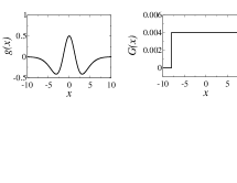
Figure 1: (Left) Kernel function of standard one-dimensional kernel-based models considering both competitive and facilitative interactions. It is built with a combination of positive and negative Gaussian functions, $g(x)=1.5\exp\left(-(x/2)^{2}\right)-\exp\left(-(x/4)^{2}\right)$. (Right) Competitive-only top-hat kernel with range $R=8$.

II.2 A kernel-based model including only competitive interactions

Following previous studies (Rietkerk & van de Koppel, 2008; Martínez-García et al., 2013b) suggesting that vegetation patterns could emerge without short-range facilitation, and assuming that competition for water is the unavoidable interaction in arid and semiarid systems, Martínez-García et al. (2013a) proposed a nonlocal model with only competitive interactions. The equation for vegetation density is

$$\frac{\partial\rho({\bf x},t)}{\partial t}=\beta_{0}r(\tilde{\rho},\delta)\rho({\bf x},t)(1-\rho({\bf x},t))-\alpha\rho({\bf x},t),$$ (2)

where $\tilde{\rho}$ is the mean vegetation density within a neighborhood, weighted with the kernel $G(x)$, around a given spatial point:

$$\tilde{\rho}({\bf x},t)=\int G(|{\bf x}-{\bf x^{\prime}}|)\rho({\bf x^{\prime}},t)d{\bf x^{\prime}}.$$ (3)

The different terms in the model come from considering the growth and death dynamics of vegetation. Population growth follows a sequence of seed production, dispersal and establishment:

1. Production happens at rate $\beta_{0}$ per plant. Assuming local seed dispersion and that all seeds may give rise to new plants, the growth rate is $\beta_{0}\rho$. After a seed lands, it has to overcome competition to establish. The two next competing mechanisms are taken into account:

2. Space availability limits the density to a maximum value $\rho_{max}$, so the proportion of available space at a point ${\bf x}$ is $1-\rho(\bf x,t)/\rho_{max}$. Density can be scaled such that $\rho_{max}=1$ and thus the growth term is limited by a factor $(1-\rho(\bf x,t))$.

3. Once the seed has germinated, it competes with other plants for water and other resources in the soil. The probability of overcoming this competition is given by $r(\tilde{\rho},\delta)$. This function decreases when $\tilde{\rho}$ increases, so that $r^{\prime}(\rho_{0},\delta)\equiv(\partial r/\partial\tilde{\rho})_{\tilde{\rho}=\rho_{0}}<0$. We assume that plants compete with other plants in their neighborhood, which is defined by a distance of the order of twice the typical root length.

It is worth stressing the difference between the function $G$ in this description and the $g$ in the previous subsection. $g$ contains the information about the interactions (cooperative when positive and competitive when negative) present in the system (Lefever & Lejeune, 1997; D’Odorico et al., 2006c). Since these are of facilitative and competitive type, the kernels are positive (at short scales) and negative (at long scales). On the contrary, $G$ is strictly positive and defines an influence region of a focal plant which is used to compute an averaged density of other plants around it. Also, nonlocal competition enters nonlinearly, at variance with Eq. (1), so that negative densities no longer appear.

Performing a linear stability analysis of the stationary solution, $\rho_{0}$, of Eq. (3) the perturbation growth rate is (see Martínez-García et al. (2013a)) for details

$$\lambda({\bf k})=-\alpha\rho_{0}\left[\frac{1}{1-\rho_{0}}-\frac{r^{\prime}(\rho_{0},\delta)}{r(\rho_{0},\delta)}\hat{G}({\bf k})\right],$$ (4)

where $\hat{G}({\bf k})$ is the Fourier transform of the kernel, $\hat{G}({\bf k})=\int G({\bf x})\exp(i{\bf k}\cdot{\bf x})d{\bf x}$.

Since $r^{\prime}<0$ equation (4) indicates that patterns may appear ($\lambda>0$) in the model when $\hat{G}(\bf k)$ takes negative values, provided that competition is strong enough. This may happen, for example, when the kernel has a finite range (an example is shown in right panel of Fig. 1), so that it is only different from zero (positive) in a finite domain around $\bf x=0$. In plant dynamics, this finite range arises naturally from the length of the roots. The model recovers the gapped and striped patterns observed in arid and semiarid landscapes. Figure 2 shows the stationary patterns obtained by integrating Eq. (13) in a patch of $10^{4}$ m² with periodic boundary conditions and a competition range of $R=8$ m. $G$ is a two-dimensional top-hat function (a cut across it will be similar to the right plot in Fig. 1) and the probability of overcoming nonlocal competition is given by

$$r(\tilde{\rho},\delta)=\frac{1}{(1+\delta\tilde{\rho})},$$ (5)

which makes$\rho_{0}$ analytically solvable. The patterns only appear if the Fourier transform of the kernel function has negative values. For the two-dimensional top hat kernel of width 2R, the Fourier transform is $\hat{G}(k)=2J_{1}(kR)/kR$, where $J_{1}$ is the first order Bessel function (Hernández-García & López, 2004).

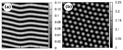
Figure 2: Close-to-stationary spatial structures shown by the model using the $r(\tilde{\rho},\delta)$ given by Eq. (5). Darker grey levels represent smaller densities. (a) Vegetation stripes, $\delta=16.0$. (b) Vegetation spots, $\delta=17.0$. Other parameters: $\beta_{0}=1.0$ and $\alpha=0.5$.

II.3 Competition through a nonlocal nonlinear death term

As a complement to the vegetation dynamics in Eq. (3) we next discuss a system, again without facilitation, where resource competition enters through the death rate. There is now a nonlocal nonlinear death term resulting in a higher death rate when the surrounding vegetation density increases. This is mathematically expressed as:

$$\frac{\partial\rho({\bf x},t)}{\partial t}=\beta\rho({\bf x},t)(1-\rho({\bf x},t))-\alpha_{d}\rho({\bf x},t),$$ (6)

where $\alpha_{d}=\alpha_{0}h(\tilde{\rho}({\bf x},t),\delta)$ is the nonlocal death rate ($\alpha_{0}$ is a constant and $h$ an arbitrary function), and $\beta$ is the constant birth rate. Nonlocal competition affecting mortality has been shown to promote clustering in individual-based population models (Birch & Young, 2006).

As before, $\tilde{\rho}({\bf x},t)$ is the nonlocal density of vegetation at the point ${\bf x}$, where $\tilde{\rho}({\bf x},t)=\int\rho({\bf x^{\prime}},t)G(|{\bf x}-{\bf x^{\prime}}|)dx^{\prime}$. $G$ is the kernel function that defines an interaction range and modulates its strength with the distance from the focal plant. Space availability for a seed to establish appears in the birth term via $1-\rho({\bf x},t)$ (local competition). $h(\tilde{\rho}({\bf x},t),\delta)$ gives the probability that a plant dies as a function of competition for water with the roots of other plants. Since it is a probability, $0<h<1$ and it increases with increasing values of the averaged density, $\bar{\rho}$, and the (positive) competition parameter, $\delta$. The stationary solutions of Eq. (6), $\rho_{0}$, are obtained by solving

$$\beta\rho_{0}(1-\rho_{0})-\alpha_{0}h(\rho_{0},\delta)\rho_{0}=0,$$ (7)

which has a trivial solution, $\rho_{0}=0$ referring to the bare-ground state, and a vegetated state that is obtained from

$$\beta(1-\rho_{0})-\alpha_{0}h(\rho_{0},\delta)=0,$$ (8)

once the function $h$ has been chosen.

A linear stability analysis of the stationary homogeneous state, $\rho_{0}$, yields the dispersion relation

$$\lambda({\bf k})=\beta(1-2\rho_{0})-\alpha h(\rho_{0},\delta)-\alpha\rho_{0}h^{\prime}(\rho_{0},\delta)\hat{G}({\bf k}),$$ (9)

where $\hat{G}({\bf k})$ is the Fourier transform of the kernel function.

The simplest function $h$ that fulfills the above-mentioned properties is a linear function, $h(\tilde{\rho},\delta)=\delta\tilde{\rho}$, which limits the values of the competition parameter to $0<\delta<1$ so that $h<1$. Then

$$\rho_{0}=\frac{\beta}{\beta+\alpha_{0}\delta},$$ (10)

while the perturbation growth rate is given by

$$\lambda({\bf k})=-\frac{\beta}{\beta+\alpha_{0}\delta}\left[\beta+\alpha_{0}\delta\hat{G}({\bf k})\right],$$ (11)

from which we obtain a transition to pattern ($\lambda$ becomes positive) at a competition strength,

$$\delta_{c}=-\frac{\beta}{\alpha_{0}\hat{G}({\bf k_{c}})},$$ (12)

where $k_{c}$ is the most unstable mode, which yields the most negative value of $\hat{G}$ and is the mode with the highest growth rate. First note that again the Fourier transform of $G$ must take negative values for patterns to form. Also, $\alpha_{0}$ and $\beta$ have to be chosen properly to have $\delta_{c}\leq 1$. In particular, if we take $\alpha_{0}=1$, $\beta=0.1$, and a top-hat kernel of radius $R=8$, we get $\delta_{c}\approx 0.75$. It is important to remark that spatial structures result when the maximum death rate, i.e., the death rate in fully vegetated areas, is much higher than the birth rate $(\alpha_{0}\gg\beta)$. Otherwise the model shows standard logistic growth despite the nonlocal spatial couplings and the distribution of vegetation is homogeneous. Figure 3 shows the different spatial distributions of vegetation in the stationary state. The homogeneous distribution is stable when $\delta<\delta_{c}$ (3a), while patterns (stripes and spots) exist for $\delta>\delta_{c}$ (3b) and (3c), respectively.

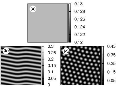
Figure 3: Distribution of vegetation produced by the model with a linear probability $h$ for different values of the competition parameter. $\delta=0.7$ (Left), $\delta=0.8$ (Center), $\delta=0.9$ (Right). $\alpha_{0}=1$, $\beta=0.1$.

II.4 Competition through a nonlocal linear death term

We next study a natural extension of the kernel based model as presented in Eq. (1) and previous studies (Borgogno et al., 2009), but with purely competitive interactions. The local density of vegetation changes in time because of its local dynamics (logistic growth) and the spatial interactions (competition) with other points in the domain,

$$\frac{\partial\rho(x,t)}{\partial t} = D\nabla^{2}\rho(x,t)+\rho(x,t)\left[1-\frac{\rho(x,t)}{\kappa}\right]$$ (13)

$$- \Omega\int G_{a}(|x-x^{\prime}|)\rho(x^{\prime},t)dx^{\prime},$$

where $\kappa$, is the carrying capacity and $\Omega$ is the interaction parameter. We have added a diffusive term modeling seed dispesal. Competitive interactions are determined by considering the strength of the interactions parameter, $\Omega$, and the kernel function, $G_{a}$, both always positive. This description is equivalent to considering a nonlocal linear death term which arises from competition among plants. As mentioned in Subsection II.1 the density can take negative values. This is a consequence of the nonlocal interactions reinforcing the death of vegetation and entering linearly on the model; these models are, therefore, mathematically ill-posed. This is a weakness that these models share with many related kernel-based models (see Subsection II.1), but which is absent when nonlocal competition enters nonlinearly. Negative densities are nonsensical from a biological point of view, so following Borgogno et al. (2009), we set $\rho(x,t)=0$ in model (13) when this occurs. The stationary solutions are $\rho_{0}=0$ (no vegetated state), and a nontrivial solution

$$\rho_{0}=(1-\Omega)\kappa,$$ (14)

that imposes a constraint on the values of $\Omega<1$.

The growth rate of the perturbations is now

$$\lambda({\bf k})=-D|{\bf k}|^{2}+1-2\kappa^{-1}\rho_{0}-\Omega\hat{G}({\bf k}),$$ (15)

and using the expression of the homogeneous steady state, $\rho_{0}$, given by Eq. (14), it becomes

$$\lambda({\bf k})=-D|{\bf k}|^{2}-1+2\Omega-\Omega\hat{G}({\bf k}).$$ (16)

There is in this model no restriction on the shape of the Fourier transform of the kernel for the appearance of patterns (note that $\Omega$ is always lower than $1$). We have numerically integrated Eq. (13) in the regime of patterned solutions and the results are shown in Figures 4(a) and 4(b) for two different values of $\Omega$. The same sequence of spatial structures is obtained as in the other models.

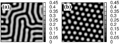
Figure 4: Spatial distribution of vegetation for the model described by Eq. (13) (a) $D=1$, $\Omega=0.7$, and (b) $D=1$, $\Omega=0.9$. $R=8$ in both panels.

III Derivation of the effective nonlocal description from tree-water dynamics

The models presented in the previous section are all given by a phenomenological evolution equation for vegetation density. An open problem is to infer this type of description from a mechanistic one where the explicit interactive dynamics of vegetation competing for water is considered. This would help, in particular, to unveil the origin and properties of the kernel function. In this section we present a preliminar (and not fully satisfactory) attempt to derive the model presented in Martínez-García et al. (2013a) and discussed in subsection II.2 (the derivation corresponding to the nonlocal death model in II.3 is a straightforward extension of this calculation).

Let us consider a system involving dimensionless vegetation density, $\rho$, and soil-water $w$. The dynamics is purely local and competitive and takes the form:

$$\partial_{t}\rho = \beta\rho(1-\rho)w-\alpha\rho,$$ (17)

$$\partial_{t}w = -\mu\rho w-\gamma w+I+D_{w}\nabla^{2}w,$$ (18)

where the nondimensional positive parameters are: the seed production rate $\beta$; the vegetation death rate $\alpha$; the consumption rate of water by vegetation, $\mu$; the evaporation rate $\gamma$, and the rainfall, $I$. Water percolation in the ground is modeled by a diffusion constant $D_{w}$. Note that this model is a simplified version, which only includes competitive interactions, of the model presented in Gilad et al. (2004).

Since the characteristic time scale of the water is much faster than the one of the biomass we can do an adiabatic elimination of the variable $w$ (i.e. $\partial_{t}w=0$) so that

$$-\mu\rho w-\gamma w+I+D_{w}\nabla^{2}w=0,$$ (19)

and thus

$$\left(D_{w}\nabla^{2}-\gamma\right)w=\mu\rho w-I,$$ (20)

whose formal solution can be obtained using Green’s functions, $G_{d}$,

$$w({\bf x})=\int G_{d}({\bf x}-{\bf s})(\mu\rho({\bf s})w({\bf s})-I)d{\bf s},$$ (21)

with the boundary conditions $w(x\rightarrow\pm\infty)=0$. For simplicity we now consider a one-dimensional situation, although analogous calculations can be done in two dimensions. The Green’s function is the solution of

$$D_{w}\partial^{2}_{{\bf x}}G_{d}-\gamma G_{d}=\delta({\bf x}-{\bf s}),$$ (22)

and it is given by

$$G_{d}({\bf x},{\bf s})=-\frac{1}{2}\exp\left(-\sqrt{\frac{\gamma}{D_{w}}}|{\bf x}-{\bf s}|\right)$$ (23)

Taking the nondimensional small number $\mu$ as the perturbative parameter, we can further obtain an approximate expression for $w$ from Eq. (21)

$$w({\bf x})=-IG_{d0}\left[1+\mu\int G_{d}({\bf x}-{\bf s})\rho({\bf s})d{\bf s}+{\cal O}({\mu^{2}})\right],$$ (24)

where $G_{d0}=\int G_{d}({\bf x}-{\bf s})d{\bf s}<0$, since the Green’s function is always negative. Plugging this in the equation for the biomass density (17), we obtain the closed expression:

$$\partial_{t}\rho=\beta\rho(1-\rho)\left\{-IG_{d0}\left[\mu\int G_{d}({\bf x}-{\bf s})\rho({\bf s})d{\bf s}+1\right]\right\}$$

$$-\alpha\rho.$$ (25)

Defining the positive nonlocal density $\tilde{\rho}=\int G_{c}({\bf x}-{\bf s})\rho({\bf s})d{\bf s}$, where $G_{c}=-G_{d}$, we can write equation (III) as

$$\partial_{t}\rho=\beta\bar{r}(\tilde{\rho})\rho(1-\rho)-\alpha\rho,$$ (26)

where we have defined $\bar{r}(\tilde{\rho})=I|G_{d0}|\left(1-\mu\tilde{\rho}\right)$.

To have a good agreement with the effective nonlocal dynamics Eq. (2), $\bar{r}>0$ since it represents a probability. This is certainly the case for small $\mu$. Note that some additional conditions on the normalization of the Green’s function have to be imposed to limit $r$ to values less than $1$. Also $\bar{r}^{\prime}(\tilde{\rho})=-I\mu|G_{d0}|$ is always negative, as we expected.

In this particular example we obtained an exponential kernel which does not have the finite-range support that would be associated to the finite root extent. As a consequence, the Fourier transform of this kernel has no negative components and then does not lead to pattern formation. The simple modeling of water dispersion by means of a diffusion constant does not contain the additional spatial scale associated to root size, and should be replaced by some mechanism implementing root effects. On the other side, the finite-range of the kernel is a sufficient but not a necessary condition for its Fourier transform to have negative values. It is well-known the existence of infinite-range kernels whose Fourier transform has negative values. This is the case of all stretched exponentials $G(x)\propto\exp({-|\bf x|^{p}})$ with $p>2$ (Pigolotti et al., 2007). Kernels satisfying this are more platykurtic than the Gaussian function. Work is in progress along this possible line to obtain pattern-forming kernels.

IV Conclusions

In this paper we have reviewed different nonlocal competitive models of vegetation in water-limited regions where, despite the absence of facilitative interactions, patterns may still appear. The obtained sequence of patterns consists on a stripped structure and spots of vegetation interspersed on the bare soil forming a hexagonal lattice. We have not been able to find patterns consisting on spots of bare soil, which are also typical in models with both competition and facilitation among plants. In fact, previous works (Martínez-García et al., 2013b) in which the range of the facilitation was taken to its infinitesimally short-range (i.e. local) shown these gapped distributions but only in a very narrow parameter region close to the transition to patterns line. This is different from standard models with nonlocal facilitation in which the whole sequence of patterns (gaps, stripes and spots) appears in a wider parameter’s interval. This may suggest that facilitative interactions, although not indispensable for the formation of patterns, could be important in order to promote some of the structures that have been reported in field observations. We note in this context that a careful study of the bifurcation sequences in local vegetation models reveals that the standard sequence is not fully robust and depends on nonlinear details of particular models (Gowda et al., 2014).

From a mathematical point of view, nonlocality enters through an influence function that determines the number of plants competing within a range with any given plant. A first-order approximation of this distance can be given by (twice) the typical length of the roots, but field measurements are needed in order to determine the the range over which individuals of a given plant species can influence their neighbors. A necessary condition for pattern transitions, for the models under study where the nonlocality is in the nonlinear term, is the existence of negative values of the Fourier transform of the influence function, which always happens, among other situations, for kernel functions with finite range.

From a biological point of view, competitive interactions alone may give rise to spatial structures because of the development of spatial regions (typically located between maxima of the plant density) where competition is stronger preventing the growth of more vegetation (Martínez-García et al., 2013a).

An unfortunate consequence of the universal character of these models is that the information it is possible to gain on the underlying biophysical mechanisms operating in the system just by studying the spatial distribution of the vegetation is limited. Many different mechanisms lead to the same patterns. Although patterns are universal, models should be specific to each system. This emphasizes the importance that empirical studies have in developing reasonable models of the behavior of different systems. Field work may help theoretical efforts by placing biologically reasonable bounds on the shape and extent of the kernel functions used in the models, and also by approximations to the probability of overcoming competition, $r(\tilde{\rho},\delta)$.

It is important to note that the type of nonlocal models presented may have localized solutions. This has been studied, in a different context (Paulau et al., 2014), for a model that reduces to Eq. (6) when the kernels enhance selfinteractions, i.e., they are of the type $G(x)=F(x)+a\delta(x)$ (Hernández-García et al., 2009). In plant ecology, mathematical approaches where the interactions among plants depend on the local biomass density show localized structures as a consequence of the bistable behavior between the desert state ($\rho_{0}=0$) and the spatially extended solutions (Lejeune et al., 2002). This result also extends to nonlocal models either considering the interplay between water and vegetation dynamics (Meron et al., 2007) or, in more recent studies using effective equations for the vegetation density (Fernandez-Oto et al., 2013). In this latter case, the authors explain the formation of fairy circles (localized barren patches of vegetation) as localized solutions of spatially non-local models.

Finally, with this work, we aimed to show that, under certain conditions, nonlocal competition alone may be responsible for the formation of patterns in semiariad systems. More interestingly, spatially regular distribution of vegetation appear regardless of how competitive interactions are introduced in the different modeling approaches. Certainly, while it may not be possible to unambiguously identify the model that generates an observed pattern, the study of the minimal mechanisms giving rise to pattern formation limits the set of candidate models (and biological mechanisms) that need to be considered. We hope that our results shed light on the task of understanding the fundamental mechanisms -and the possible absence of facilitation- that could be at the origin of pattern formation in semiarid systems.

References

- Barbier et al. (2008) Barbier, N., Couteron, P., Lefever, R., Deblauwe, V. & Lejeune, O. 2008 Spatial decoupling of facilitation and competition at the origin of gapped vegetation patterns. Ecology, 89(6), 1521–31.
- Birch & Young (2006) Birch, D. a. & Young, W. R. 2006 A master equation for a spatial population model with pair interactions. Theoretical population biology, 70(1), 26–42. (doi:10.1016/j.tpb.2005.11.007)
- Borgogno et al. (2009) Borgogno, F., D’Odorico, P., Laio, F. & Ridolfi, L. 2009 Mathematical models of vegetation pattern formation in ecohydrology. Reviews of Geophysics, 47(1), 1–36. (doi:10.1029/2007RG000256.Ecohydrology)
- D’Odorico et al. (2006a) D’Odorico, P., Laio, F. & Ridolfi, L. 2006a Patterns as indicators of productivity enhancement by facilitation and competition in dryland vegetation. Journal of Geophysical Research: Biogeosciences, 111, G03 010. (doi:10.1029/2006JG000176)
- D’Odorico et al. (2006b) D’Odorico, P., Laio, F. & Ridolfi, L. 2006b Vegetation patterns induced by random climate fluctuations. Geophysical Research Letters, 33(19), L19 404.
- D’Odorico et al. (2006c) D’Odorico, P., Laio, F. & Ridolfi, L. 2006c Vegetation patterns induced by random climate fluctuations. Geophysical Research Letters, 33(19), L19 404. (doi:10.1029/2006GL027499)
- Dunkerley (2002) Dunkerley, D. L. 2002 Infiltration rates and soil moisture in a groved mulga community near Alice Springs, arid central Australia: evidence for complex internal rainwater redistribution in a runoff-runon landscape. J Arid Environ, 51(2), 199–202.
- Fernandez-Oto et al. (2013) Fernandez-Oto, C., Tlidi, M., Escaff, D. & Clerc, M. 2013 Strong interaction between plants induces circular barren patches: fairy circles. arXiv preprint arXiv:1306.4848.
- Gilad et al. (2004) Gilad, E., von Hardenberg, J., Provenzale, a., Shachak, M. & Meron, E. 2004 Ecosystem Engineers: From Pattern Formation to Habitat Creation. Physical Review Letters, 93(9), 098 105. (doi:10.1103/PhysRevLett.93.098105)
- Gowda et al. (2014) Gowda, K., Riecke, H. & Silber, M. 2014 Transitions between patterned states in vegetation models for semi-arid ecosystems. Physical Review E, 89, 022701. (doi:10.1103/PhysRevE.89.022701)
- Hernández-García & López (2004) Hernández-García, E. & López, C. 2004 Clustering, advection, and patterns in a model of population dynamics with neighborhood-dependent rates. Phys. Rev. E, 70, 016 216. (doi:10.1103/PhysRevE.70.016216)
- Hernández-García et al. (2009) Hernández-García, E., López, C., Pigolotti, S. & Andersen, K. H. 2009 Species competition: coexistence, exclusion and clustering. Philosophical transactions. Series A, Mathematical, physical, and engineering sciences, 367(1901), 3183–95. (doi:10.1098/rsta.2009.0086)
- Klausmeier (1999) Klausmeier, C. A. 1999 Regular and Irregular Patterns in Semiarid Vegetation. Science, 284(5421), 1826–1828. (doi:10.1126/science.284.5421.1826)
- Lefever & Lejeune (1997) Lefever, R. & Lejeune, O. 1997 On the origin of tiger bush. Bulletin of Mathematical Biology, 59(2), 263–294.
- Lejeune & Tlidi (1999) Lejeune, O. & Tlidi, M. 1999 A model for the explanation of vegetation stripes (tiger bush). Journal of Vegetation Science, 10(2), 201–208. (doi:10.2307/3237141)
- Lejeune et al. (2002) Lejeune, O., Tlidi, M. & Couteron, P. 2002 Localized vegetation patches: A self-organized response to resource scarcity. Physical Review E, 66(1), 010 901. (doi:10.1103/PhysRevE.66.010901)
- Lefever & Turner (2012) Lefever, R. & Turner, J. W. 2012 A quantitative theory of vegetation patterns based on plant structure and the non-local FKPP equation. Comptes Rendus Mécanique, 340(11), 818–828.
- Martínez-García et al. (2013a) Martínez-García, R., Calabrese, J. M., Hernandez-Garcia, E. & Lopez, C. 2013a Vegetation pattern formation in semiarid systems without facilitative mechanisms. Geophysical Research Letters, 40, 6143–6147.
- Martínez-García et al. (2013b) Martínez-García, R., Calabrese, J. M. & López, C. 2013b Spatial patterns in mesic savannas: The local facilitation limit and the role of demographic stochasticity. Journal of theoretical biology, 333, 156–165. (doi:10.1016/j.jtbi.2013.05.024)
- Meron et al. (2007) Meron, E., Yizhaq, H. & Gilad, E. 2007 Localized structures in dryland vegetation: forms and functions. Chaos, 17(3), 037 109. (doi:10.1063/1.2767246)
- Murray (2002) Murray, J. 2002 Mathematical Biology. Vol I: An Introduction. Berlin, Heidelberg: Springer, 3rd edn.
- Paulau et al. (2014) Paulau, P., Gomila, D., López, C. & Hernández-García, E. 2014 Self-localized states in species competition. Physical Review E, 89, 032724 (1-8).
- Pigolotti et al. (2007) Pigolotti, S., López, C. & Hernández-García, E. 2007 Species Clustering in Competitive Lotka-Volterra Models. Physical Review Letters, 98(25), 258 101.
- Rietkerk et al. (2002) Rietkerk, M., Boerlijst, M. C., van Langevelde, F., HilleRisLambers, R., van de Koppel, J., Kumar, L., Prins, H. H. & de Roos, A. M. 2002 Notes and Comments: Self-Organization of Vegetation in Arid Ecosystems. The American Naturalist, 160(4), 534–530.
- Rietkerk & van de Koppel (2008) Rietkerk, M. & van de Koppel, J. 2008 Regular pattern formation in real ecosystems. Trends in ecology & evolution, 23(3), 169–175.
- von Hardenberg et al. (2001) von Hardenberg, J., Meron, E., Shachak, M. & Zarmi, Y. 2001 Diversity of Vegetation Patterns and Desertification. Physical Review Letters, 87(19), 198 101–. (doi:10.1103/PhysRevLett.87.198101)