Optimal Sharing Rule for a Household
with a Portfolio Management Problem

Abstract

We study an intra-household decision process in the Merton financial portfolio problem. This writes as an optimal consumption-investment problem in finite horizon for the case of two separate consumption streams and a shared final wealth, in a linear social welfare setting. We show that the aggregate problem for multiple agents can be linearly separated in multiple optimal single agent problems given an optimal sharing rule of the initial endowment. Consequently, an explicit closed form solution is obtained for each subproblem, and for the household as a whole. We show the impact of asymmetric risk aversion and market price of risk on the sharing rule in a specified setting with mean-reverting price of risk, with numerical illustration.

Keywords: Portfolio optimization; household decision; optimal consumption; martingale techniques.

JEL: G11 (primary); C61 (secondary)

1 Introduction

An important dimension of household savings decisions is the possibility of individual consumption streams out of the common wealth. In the standard household economics literature, e.g., [2, 1], the decision is most impacted by arbitrage with individual incomes. It has already been argued in [19] that the household—as a risk-sharing institution—considers personal savings as contribution to a group insurance, and that ignoring intra-household risk sharing introduces a bias in the response of savings to income shocks. In the present paper, we take a drastically different stand from the literature by focusing exclusively on the management of savings. The goal of this paper is more precisely to study the impact of heterogeneous preferences within the household on portfolio initial allocation, in a complex and dynamic financial world.

General intra-household decision problems constitute a well-known challenge. It is acknowledged that bargaining concepts (Nash style or Kalay-Smorodinsky, see [16]) are not the only ”collective” decision process alternative to modeling the household as a single decision unit. In his seminal contribution, Chiappori [4] minimally defines collective rationality by simply requiring the household to be on the Pareto-efficient frontier. This notably leads the household to derive, in his respective labor-consumption problem, an income sharing rule based on the common initial endowment. He [5] then shows in that setting that household decisions are efficient if and only if some sharing rule exists. Obtaining such a rule is our objective, in a very specific context: the Merton portfolio problem.

The optimal investment problem is much more involved than a static labor-consumption allocation, for at first it is dynamical. Obtaining the initial sharing rule is only the first step of solving the economic problem: explicit the financial strategy and the optimal consumption path are necessary to fully understand intra-household decisions, in time. In a dynamic extension of [4, 5], Mazzocco [17] underlines that household decisions must be specified to be under some commitment or non-commitment paradigm: if the evolution of members endowments moves away from the sharing rule, anticipation of that fact must be taken into present negotiation. Under commitment, members sticks to the sharing rule while without it, the solution involves a game-theoretic approach. See also [6] for a recent review on that topic. For the sake of simplicity, we remain under the commitment assumption. Yet in the easiest setting, the problem remains difficult if the intra-household interactions are not specified. That is why we set the problem for a linear household Welfare function based on separable Von-Neuman Morgenstern utility preferences. As we obtain the optimal sharing rule in this setting (see Theorem 4.4 hereafter), we are inclined to conjecture ex-post that some collective rationality arises from it (see in particular [4], p. 74).

How does the problem writes? Specifically, the household (e.g. spouses) involves two separated utility functions $U_{1}$ and $U_{2}$ for consumption streams of money $c^{1}$ and $c^{2}$ respectively, and two distinct (non necessarily constant nor equal) discount rates $\beta^{1}$ and $\beta^{2}$ to measure their individual impatience. Additionally, since we consider problem in finite horizon $T$, they share a common utility function $U_{3}$ to evaluate together the resulting terminal wealth $X_{T}$, discounted with rate $\beta^{3}$. This wealth is obtained as the result of a financial portfolio strategy on the time interval $[0,T]$, starting from an initial endowment $X_{0}=x$ and invested in risky or riskless assets. We pose the problem of maximizing

$$\mathbb{E}\left[\int_{0}^{T}e^{\left(-\int_{0}^{t}\beta^{1}(s)ds\right)}U_{1}(c_{t}^{1})dt+\int_{0}^{T}e^{\left(-\int_{0}^{t}\beta^{2}(s)ds\right)}U_{2}(c_{t}^{2})dt+e^{\left(-\int_{0}^{T}\beta^{3}(s)ds\right)}U_{3}(X_{T})\right]\;,$$ (1.1)

by choosing the optimal consumption rates $(c^{i}_{t})_{t\in[0,T]}$ for $i=1,2$ and the portfolio allocation $(X_{t})_{t\in[0,T]}$. Having now sketched the mathematical problem, we may comment on it from different standpoints.

It is important to understand that the portfolio is a self-financing portfolio, i.e., it starts with a given initial wealth and does not undergo any additional injection of savings. The fundamental factors influencing the sharing rule will thus be risk aversion embedded in utility functions, and impatience in individual discount rates. Our contribution mainly attempt to provide the sharing rule regarding those typical financial dimensions, that is, when members of the household have different levels of risk aversion or impatience. In this respect, our article really stands as a contribution to the portfolio management literature.

But in the later research field, problem (1.1) is relatively new. In the classical portfolio management problem, the single agent model is the default representation. It has already been argued [22] that consumption and terminal wealth should be evaluated distinctly, as the nature of the reward is different (empirical works [18] highlight a greater risk aversion toward consumption than toward wealth). In [22], Six makes that distinction, yet for a single agent. He shows, as we do, the separability of the problem, and that the allocation of money to consumption (the consumption satisfaction proportion, or CSP) drastically depends—but monotonously—on the initial wealth. By introducing two separate consumption streams, we go further than Six [22], since there is an intricate dependence of each consumption stream with the common resulting wealth. We show that our model, unlike the one of [22], can exhibit a hump shaped consumption satisfaction proportion.

What other insights do we learn from this model? We end the paper with a numerical application with closed form solutions based on the consumption-savings problem of Wachter [23]. Especially, we show that the previously mentionned consumption satisfaction proportion increases with the initial endowment, but slower for the more risk averse agent. When the initial endowment is large enough, the less risk averse agent allocates relatively more money to future consumption. This mainly shapes the initial sharing rule, as expected. This allows us to study consumption satisfaction proportion dependence with respect to the market price of risk and risk aversion. The numerical results revealed that, unlike the effect of market price of risk change which is marginal, a change in risk aversion can significantly impact the consumption satisfaction proportion. Those intuitions, developed in Section 5, are for the benefit of portfolio managers. As we mentioned it a the very beginning, we acknowledge that the study of a household financial portfolio problem is at odd with existing literature focusing on labor-consumption-leisure arbitrage, and that few household data would be available to help reveal the pertinence of the implemented setting. Nevertheless, the application seems much more realistic when one thinks of the situation of a mutual fund portfolio manager working for a pool of heterogeneous clients, or in the framework of a hedge fund optimal dividend distribution from the shareholders perspective. If household decision theory is our starting point to introduce the problem, the applications are more numerous in the financial industry. We comment shortly in the paper on the possibility to extend the setting to $n>2$ consumption streams. The reader will easily be able transpose te present results to a much larger pool of agents.

The remainder of the article is organized as follows. Section 2 introduces the financial market, assumed to be complete, portfolios and their properties. Section 3 develops the central theorem, i.e., the optimal initial sharing rule. Accordingly, the problem can be separated in three subproblems which are solved explicitely via classical duality techniques, see [13]. We comment also on how [22] extends non trivially from one to two agents, and how to extend the setting to more than two. Section 5 presents the specific case based on power utility functions and a mean reverting price of risk, first introduced in [23].

2 The financial market and portfolio properties

2.1 A complete financial market

We start by describing the dynamics of asset prices. We consider a classical framework of a complete financial market in continuous time, with one riskless asset $S^{0}$ (a bank account) and $d$ risky assets $(S^{1},\ldots,S^{d})$, i.e. stocks. It is important to notice that the methodology we developed does not extend naturally to incomplete markets. This is because of the non uniqueness of the martingale measure, which would forbid to uniquely define the utility price of risks.

The riskless asset will evolve at the interest rate $(r_{t})_{t\in[0,T]}$, that is,

$$dS^{0}_{t}=r_{t}S^{0}_{t}dt\;,\quad 0\leq t\leq T\;,$$

with $S^{0}_{0}=s_{0}$. To model risky assets, we consider a filtered probability space $(\Omega,\mathcal{F},\mathbb{P})$ supporting a standard $d$-dimensional Brownian motion $W:=(W_{t})_{t\in[0,T]}=(W^{1}_{t},\ldots,W^{d}_{t})^{T}_{t\in[0,T]}$. As it is usually assumed, the filtration $(\mathcal{F}_{t})_{t\in[0,T]}$ is the augmentation under $\mathbb{P}$ of the natural filtration of $W$. The risky assets then follow a generalized Black-Scholes model (an Itô diffusion process):

$$dS^{i}_{t}=S^{i}_{t}\left(b_{i}(t)dt+\sum_{j=1}^{d}\sigma_{ij}(t)dW_{t}^{j}\right)\;,\quad 0\leq t\leq T\;,$$ (2.1)

with $(S^{1}_{0},\ldots,S^{d}_{0})=(s_{1},\ldots,s_{d})\in(0,\infty)^{d}$. The vector of mean rates of return
$b(t):=(b_{1}(t)\ldots b_{d}(t))^{T}_{t\in[0,T]}$ and the diffusion matrix $\sigma(t):=(\sigma_{ij}(t))_{1\leq i,j\leq d,t\in[0,T]}$ are assumed to be adapted to the filtration $\mathcal{F}$. Moreover, $\sigma(t)$ is assumed to be invertible for all $t$. The interest rate process $(r(t))_{t\in[0,T]}$ can also be made stochastic if it is assumed to be adapted. We assume that $b$, $\sigma$ and $r$ are such that the stochastic differential equation (2.1) has a unique strong solution

As usual, we use the riskless asset as a numéraire and replace asset prices by their discounted counterpart. The discount factor is defined by

$$D_{t}:=\exp\left(-\int_{0}^{t}r(u)du\right)\;,\quad 0\leq t\leq T\;.$$ (2.2)

and for a generic process $Y_{t}$, $\tilde{Y}_{t}:=Y_{t}D_{t}$ denotes the discounted version.

Importantly, we assume that the financial market is complete, in the sense of [9]. It will mean that no arbitrage is possible on the market and that utility price of risks can be uniquely determined. It is defined in our setting by the existence of a unique $\mathbb{P}$-equivalent martingale measure $\tilde{\mathbb{P}}$. If we define the price of risk process $\theta(t):=\sigma(t)^{-1}(b(t)-r(t){\mathbf{1}})$, for $t\in[0,T]$, then market completeness translates into some integrability conditions on $\theta$, so that $\tilde{W_{t}}:=W_{t}+\int_{0}^{t}\theta(s)ds$ is a Brownian motion under $\tilde{\mathbb{P}}$, see [14]. We set $\tilde{\mathbb{E}}$ the expectation operator under $\tilde{\mathbb{P}}$. We can also specify the Radon Nikodym derivative process of $\tilde{\mathbb{P}}$ w.r.t. $\mathbb{P}$ as the process

$$Z_{t}:=\exp\left\{-\sum_{i=1}^{d}\int_{0}^{t}\theta_{i}(s)dW_{s}^{i}-\frac{1}{2}\int_{0}^{t}||\theta(s)||^{2}ds\right\}\;,\quad\text{ for }t\in[0,T]\;.$$ (2.3)

A sufficient condition for market completeness to hold is that the process $(Z_{t})_{t\in[0,T]}$ is a (true) $\mathbb{P}$-martingale. We thus assume the latter throughout the paper. Sufficient conditions for $Z$ to be a martingale are Novikov and Kazamaki conditions [14]. If the process $\theta(t),t\in[0,T]$ is Markovian, [24] provide finer sufficient conditions. Those are not the concern of this paper.

2.2 Admissible portfolios

The above framework has been considered by [13] for a single investor and [22] focused on the special case of an investor with two different power utilities: one for consumption and one for final wealth. We consider here two consumption streams and one common terminal portfolio value evaluation. We comment the generalization to an arbitrary number of consumption streams and terminal values in subsection 3.3.

Our first concern is to represent the asset allocation. For that purpose we define a portfolio strategy as a $\mathcal{F}$-adapted $\mathbb{R}^{d}$-valued process $\pi:=\{\pi(t)=(\pi_{1}(t),\ldots,\pi_{d}(t))^{\top}\}$, where $\pi_{i}(\omega)\in L^{2}([0,T])$ for $\mathbb{P}$-almost every $\omega\in\Omega$. The interpretation is natural: for $i=1,\ldots,d$, $\pi(t)$ denotes the number of shares of asset $i$ held in the portfolio at time $t$.

We then introduce consumption streams as $\mathcal{F}$-adapted processes $(c_{t}^{1},c_{t}^{2})_{t\in[0,T]}$. They are assumed to take non-negative values and be such that $C(\omega):=c^{1}(\omega)+c^{2}(\omega)$ is in $L^{1}([0,T])$ for $\mathbb{P}$-almost every $\omega\in\Omega$.

The corresponding wealth process $X:=(X_{t})_{t\in[0,T]}$ is uniquely defined by

$$X_{t}=\frac{1}{D(t)}\left(x+\int_{0}^{t}\left(\left(\pi^{T}(s)b(s)-C_{s})\right)D(s)ds+\pi^{T}(s)\sigma(s)D(s)dW_{s}\right)\right),$$ (2.4)

or equivalently by the discounted version

$$\tilde{X}_{t}=\left(x+\int_{0}^{t}\left(\left(\tilde{\pi}^{T}(s)b(s)-\tilde{C}_{s})\right)ds+\tilde{\pi}^{T}(s)\sigma(s)dW_{s}\right)\right)\;.$$ (2.5)

Definition 2.1.

A triplet $(\pi,c^{1},c^{2})$ of strategy and consumption processes is said to be admissible for the initial endowment $x\geq 0$ if the corresponding wealth process $X_{t},t\in[0,T]$ satisfies $X_{t}\geq 0$ for $[0,T]$ $\mathbb{P}$-a.s. We call $A(x)$ the class of admissible processes $(\pi,c^{1},c^{2})$ for initial wealth $x$, and $P(x)$ the subset of $A(x)$ composed of triplets of the form $(\pi,0,0)$.

The set $P(x)$ describes self-financed portfolio strategies in the usual sense.

2.3 Supermartingale properties

Using standard results, we develop here intutions on how the portfolio and consumption will be managed if the problem (1.1) can be separated in three. The results below are mostly technical and can be skipped at first reading.

Admissibility of strategies can be expressed as a no-arbitrage or martingale property. Indeed, one can write equation (2.4) under $\tilde{\mathbb{P}}$:

$$\tilde{X}_{t}+\int_{0}^{t}\tilde{C}_{s}ds=x+\int_{0}^{t}\tilde{\pi}^{T}(s)\sigma(s)d\tilde{W}(s)\;,$$ (2.6)

and notice that if the corresponding triplet $(\pi,c^{1},c^{2})$ is admissible, then the left-hand side of (2.6) is non negative, and the right-hand side is a local martingale under $\tilde{\mathbb{P}}$. It follows that the left-hand side, and hence also $\tilde{X}_{t}$, is a non negative super-martingale under $\tilde{\mathbb{P}}$. Now, if $\tau_{0}:=T\wedge\inf\{0\leq t\leq T,X_{t}=0\}$, then $X_{t}=0$ for all $t\in[\tau_{0},T]$ on $\{\tau_{0}>-\infty\}$. The super martingale property in (2.6) yields

$$\tilde{\mathbb{E}}\left[\tilde{X}_{T}+\int_{0}^{T}\tilde{C}_{t}dt\right]\leq x\;.$$ (2.7)

An immediate intuition is that after applying the sharing rule on the initial endowment, a portfolio dedicated to consumption of one or the other member of the household, being assigned her initial endowment, should optimally end with no wealth at all. We thus introduce for any $x>0$ the set $C(x)$ as the set of consumption streams $c(t)$ such that

$$\tilde{\mathbb{E}}\left[\int_{0}^{T}\tilde{C}_{t}dt\right]\leq x\;;$$ (2.8)

and $D(x)$ the subset of $C(x)$ when equality holds. By linearity of the expectation, $C=c^{1}+c^{2}\in C(x_{1}+x_{2})$ if $c^{1}\in C(x_{1})$ and $c^{2}\in C(x_{2})$ (and the same by replacing with the sets $D$). The wealth process $X$ corresponding to any $C\in D(x)$ satisfies

$$X_{t}=\tilde{\mathbb{E}}\left[\int_{t}^{T}\tilde{C}_{s}ds|\mathcal{F}_{t}\right],\quad 0\leq t\leq T\;.$$ (2.9)

In particular, $X_{T}=0$ $\mathbb{P}$-a.s., as foresaw. We implicitely use expression (2.9) to construct a portfolio from a consumption process.

Similarly for the final wealth, we define $L(x)$ (resp. $M(x)$) the class of non negative random variables $L$ on $(\Omega,\mathcal{F}_{T},\tilde{\mathbb{P}})$ which satisfy

$$\tilde{\mathbb{E}}\left[L\right]\leq x\ \left(\text{ resp. }=x\right)\;.$$ (2.10)

As shown in [22] by applying the martingale representation theorem, we can construct a portfolio strategy $\pi$ for every given $c^{1}+c^{2}\in C(x)$, such that $(\pi,c^{1},c^{2})\in A(x)$. Again, we can avoid explicating $\pi$ which is deduced from other quantities. The set $C(x)$ consists of exactly those “reasonable” consumption processes, for which the couple of investors, starting out with wealth $x$, is able to construct an admissible portfolio.

Reciprocally for every $L\in L(x)$ there exists a trio $(\pi,c^{1},c^{2})\in A(x)$, which can be explictely constructed (see [22]), with corresponding wealth process $X$, for which $X_{T}=L$ $\mathbb{P}$-a.s. Specifically there exists a portfolio strategy $\pi\in P(x)$ with corresponding wealth process

$$X_{t}=\tilde{\mathbb{E}}[L|\mathcal{F}_{t}],\quad\text{ for\; }t\in[0,T].$$ (2.11)

Thus, the extreme elements of $L(x)$ (i.e., in $M(x)$) are attainable by strategies that mandate zero consumption. Indeed according to (2.6), the set $P(x)$ corresponds to strategies such that $X_{T}$ belongs to $M(x)$. From now on it will be more convenient to invoke the wealth process $X$ rather than the precise portfolio strategy $\pi$ that needs to be implemented to obtain the former.

In the admissible case, $X_{T}\geq 0$ and $C_{t}\geq 0$ for all $t\in[0,T]$. Thus, $(\pi,c^{1},c^{2})\in A(x)$ implies $c^{1},+c^{2}\in C(x)$, and $X_{T}\in L(x)$ implies inequality condition (2.8) which, together with (2.10), turns out to be also sufficient for admissibility.

3 The household problem

3.1 Risk aversion, impatience and additional elements

Each member of the household is endowed with a utility function $U_{i}$ for $i=1,2$ applied to consumption streams, and they share a common utility $U_{3}$ for the final wealth. All three functions satisfy the following assumption.

Assumption 3.1.

The function $x\mapsto U(x)$ is a strictly increasing, strictly concave real-valued function in $C^{2}([0,\infty])$ such that $x\mapsto U^{\prime\prime}(x)$ is non decreasing, $U(0)\geq-\infty$ and $U^{\prime}(\infty)=0$.

Assumption 3.1 designates a class of functions which includes CARA and HARA utility functions. Let us drop the $i$ notation for the moment, as what follows stands for the three functions under Assumption 3.1.

Under Assumption 3.1, a marginal utility $U^{\prime}$ is defined from $[0,\infty)$ onto $[0,U(0)]$. We denote $I:=(U^{\prime})^{-1},$ the inverse functions of the marginal utility (later indexed with $i=1,2,3$). Note that we allow for $U(0)=-\infty$ or $U^{\prime}(0)=\infty$. Because $U^{\prime}:[0,\infty]\rightarrow[0,U^{\prime}(0)]$ is strictly decreasing, it has a strictly decreasing inverse $I:[0,U^{\prime}(0)]\rightarrow[0,\infty]$. We extend $I$ to be a continuous function on the entirety of $[0,\infty]$ by setting $I(y)=0$ for $U^{\prime}(0)\leq y\leq\infty$, and note that

$$U(I(y))\geq U(c)+yI(y)-yc,\;\text{for}\;(y,c)\in(0,\infty)\times[0,\infty)\;.$$ (3.1)

This equation will turn to be essential in order to apply duality results in the flavor or [13].

To each utility valuation corresponds a discount rate $\beta^{i}$ assumed to be $\mathcal{F}$-adapted and bounded for all $t$ uniformly $\mathbb{P}$-almost surely. An important triplet of processes for later are the state price processes $\zeta^{i}$ which depend on the discount rates for $i=1,2,3$:

$$\zeta_{t}^{i}:=Z_{t}D_{t}\exp\left(\int_{0}^{t}\beta^{i}(u)du\right)=\frac{\tilde{Z}_{t}}{B_{t}^{i}}\;.$$

where the process $Z_{t},t\in[0,T]$ is the Radon Nikodym process given by (2.3), $D_{t}$ the market discount factor from (2.2), and

$$B^{i}_{t}:=\exp\left(-\int_{0}^{t}\beta^{i}(s)ds\right),\quad i=1,2,3$$ (3.2)

are notations for the discount factors for their respective utility functions. Recall now the general discount factor process $(D_{t})_{t\in[0,T]}$, for it is used in the definition of the following functions defined on $\mathbb{R}_{+}$:

$$\mathcal{H}_{i}(y):=\tilde{\mathbb{E}}\left[\int_{0}^{T}D_{u}I_{i}(y\zeta_{u}^{i})du|\mathcal{F}_{t}\right]\;\text{for }\;i=1,2\;,$$ (3.3)

and

$$\mathcal{H}_{3}(y):=\tilde{\mathbb{E}}\left[D_{T}I_{3}(y\zeta_{T}^{3})|\mathcal{F}_{t}\right]\;.$$ (3.4)

Assumption 3.2.

The functions $\mathcal{H}_{i}$ are finite, i.e. for all $y\in(0,\infty)$ and $i=1,2,3$, $\mathcal{H}_{i}(y)<\infty$.

The $\mathcal{H}_{i}$ functions basically stand for the dual functions, which associate a monetary worth to a utility level $y$, discounted and expected properly, and play a determinant role in fixing the sharing rule below.

Lemma 3.3.

For $i=1,2,3$, $\mathcal{H}_{i}$ is a continuous function, strictly decreasing on $(0,\infty)$ with $\mathcal{H}_{i}(0)=\infty$ and $\mathcal{H}_{i}(\infty)=0$

The above Lemma is proved in [13]. Since the above functions are strictly monotonous as well and we can define $\mathcal{Y}_{i}:=\mathcal{H}_{i}^{-1}$ the inverse of the function $\mathcal{H}_{i}$ for $i=1,2,3.$ Let us notice that $\mathcal{Y}_{i}:[0,\infty]\rightarrow[0,\infty]$. We now have properly introduced the dual elements for each problem. We end this section by introducing a technical assumption about them.

Assumption 3.4.

For all $y\in(0,\infty)$,

$$\mathbb{E}\left[\int_{0}^{T}B_{t}^{1}|U_{1}(I_{1}(y\zeta_{t}^{1}))|dt+\int_{0}^{T}B_{t}^{2}|U_{2}(I_{2}(y\zeta_{t}^{2}))|dt+B_{T}^{3}|U_{3}(I_{3}(y\zeta_{T}^{3}))|\right]<\infty\;.$$

Furthermore assume that the functions

$$y\mapsto\mathbb{E}\left[\int_{0}^{T}B_{t}^{i}|U_{i}(I_{i}(y\zeta_{t}^{1}))|dt\right],\,\,\,i=1,2,\quad y\mapsto\mathbb{E}B_{T}^{3}|U_{3}(I_{3}(y\zeta_{T}^{3}))|,$$

are differentiable and the derivatives with respect to $y$ can be taken under the expectation and integral signs.

For example, this assumption translates into the finitness of nth order moment of the process $Z$ defined in (2.3), when utilities are of the nth power type. All the above assumptions are therefore purely technical and are attributable to agents’ preferences.

3.2 Value functions

We now formalize the main problem (1.1). According to definitions (3.2), we can now rewrite (1.1) as the objective function

$$J(x;\pi,c^{1},c^{2}):=E\left[\int_{0}^{T}(B^{1}_{t}U_{1}(c_{t}^{1})+B^{2}_{t}U_{2}(c_{t}^{2}))dt+B^{3}_{T}U_{3}(X_{T})\right].$$

To our optimization problem, and for a given initial wealth $x>0$ shared by the agents, we can associate the value function

$$V(x):=\sup\limits_{(\pi,c^{1},c^{2})\in\tilde{A}(x)}J(x;\pi,c^{1},c^{2})\;,$$ (3.5)

where the set $\tilde{A}(x)$ is a subset of $A(x)$ defined simply to ensure that the expectation, that is

$$\tilde{A}(x):=\left\{(\pi,c^{1},c^{2})\in A(x):|J(x;\pi,c^{1},c^{2})|<\infty\right\}.$$

Notice that for any $x>0$, $\tilde{A}(x)=A(x)$ as soon as $U_{i}(0)>-\infty$ for $i=1,2,3$. From now on we will exclusively focus on admissible triplets in $\tilde{A}(x)$.

For a twice differentiable function $V$, we recall that the relative risk aversion is defined by

$$x\mapsto R(x):=-\frac{xV^{\prime\prime}(x)}{V^{\prime}(x)}\;.$$ (3.6)

Anticipating theorem 4.4 below—that an optimal sharing rule exists—we define the value functions associated to the three sub-problems relative to the three respective utilities. For a given $x$, which is now the personal endowment following from the sharing rule, let $V_{1}$ be the value function

$$V_{1}(x):=\sup\limits_{(\pi^{1},c^{1})\in A_{1}(x)}J_{1}(x;\pi^{1},c^{1})=\sup\limits_{(\pi^{1},c^{1})\in A_{1}(x)}E\left[\int_{0}^{T}B^{1}_{t}U_{1}(c_{t}^{1})dt\right]$$ (3.7)

with $A_{1}(x):=\left\{(\pi^{1},c^{1}):(\pi^{1},c^{1},0)\in A(x)\text{ and }|J_{1}(x;\pi^{1},c^{1})|<\infty\right\}\;.$ The value function $V_{2}$ and the set $A_{2}(x)$ for all $x>0$ are defined in a strictly similar fashion. For the terminal wealth, we set

$$V_{3}(x):=\sup\limits_{\pi^{3}\in P(x)}J_{3}(x;\pi^{3})=\sup\limits_{\pi^{3}\in P(x)}E\left[\int_{0}^{T}B^{3}_{t}U_{3}(X_{T})dt\right]$$ (3.8)

Notice that we conveniently use subsets of $A(x)$ ($A_{1}(x),A_{2}(x)$ and $P(x)$) to facilitate aggregation.

3.3 Extensions

Our model can be easily extends to more than two consuming agents. The extension to more than one evaluation of the terminal wealth is however a matter of definition. The function $J$ is indeed defined with only one portfolio strategy and one terminal value: the linearity of $X_{t}$ in the financial strategy $\pi_{t}$ allows to separate into three sub-problems as asserted by Theorem 4.4. However, changing the third term in the objective function $J$ for a term like

$$\mathbb{E}\left[e^{\left(-\int_{0}^{T}\beta^{1}(s)ds\right)}U_{4}(X^{1}_{T})+e^{\left(-\int_{0}^{T}\beta^{2}(s)ds\right)}U_{5}(X^{2}_{T})\right]\;,$$

implies to define how agents $1$ and $2$ proceed. If they share an initial wealth, a common portfolio, and decide at $T$ to split the final wealth, then the problem is strictly equivalent to (3.5) with $\beta^{3}=0$ and

$$U_{3}(x):=\sup_{\epsilon\in[0,1]}e^{\left(-\int_{0}^{T}\beta^{4}(s)ds\right)}U_{4}(\epsilon x)+e^{\left(-\int_{0}^{T}\beta^{5}(s)ds\right)}U_{5}((1-\epsilon)x)\;.$$

If one wants to distinguish agents portfolios, then he shall redefine $J$ in order to separate trading portfolios and consumption portfolios from $t=0$. The problem can be solved by using the value function approach of Theorem 4.4.

The utilities of the two agents consumption and the utility of the final wealth can be aggregated by Pareto weights. These weights are a reflection of the bargaining power of the two agents. In this case, for a given $x>0$, we define the value function $V$ evaluated at $x,$ i.e., $V(x)$ by

$$V(x):=\sup\left\{J(x;\pi,c^{1},c^{2}):(\pi,c^{1},c^{2})\in\tilde{A}(x)\right\}\;,$$ (3.9)

where

$$J(x;\pi,c^{1},c^{2}):=E\left[\int_{0}^{T}\mu^{1}(t)B^{1}_{t}U_{1}(c_{t}^{1})+\mu^{2}(t)B^{2}_{t}U_{2}(c_{t}^{2}))dt+(1-\mu^{1}(t)-\mu^{2}(t))B^{3}_{T}U_{3}(X_{T})\right].$$

Here $\mu^{1}(t),\mu^{2}(t)$ are Pareto weights in $[0,1]$ and $t\in[0,T].$ Equation above can be rewritten as

$$J(x;\pi,c^{1},c^{2}):=E\left[\int_{0}^{T}\bar{B}^{1}_{t}U_{1}(c_{t}^{1})+\bar{B}^{2}_{t}U_{2}(c_{t}^{2}))dt+\bar{B}^{3}_{T}U_{3}(X_{T})\right],$$

with

$$\bar{B}^{i}_{t}:=\exp\left(-\int_{0}^{t}\bar{\beta}^{i}(s)ds\right),\quad i=1,2,3,$$ (3.10)

and $\bar{\beta}^{i}(t),\,t\in[0,T],\,i=1,2,3$ appropriately chosen.

4 Solution to the problem

We start by solving problem (3.7) in subsection 4.1, and follow with problem (3.8) in subsection 4.2. The optimal sharing rule and the relation with problem (3.5) are then presented in subsection 4.3, problem (3.5) being solved at this moment.

4.1 Solving optimal consumption problems

We hereby solve the problem (3.7) by naturally extending the solution to the other household member. The setting and the assumptions especially allow to elicitate the explicit optimal consumption path.

Proposition 4.1.

Let $x_{1}\geq 0$. Then $V_{1}(x_{1})=J_{1}(x_{1};\boldsymbol{\pi}^{\mathbf{1}}(x_{1}),\mathbf{c}^{\mathbf{1}}(x_{1}))$ where for all $t\in[0,T]$,

$$\mathbf{c}^{\mathbf{1}}_{t}(x_{1}):=I_{1}(\mathcal{Y}_{1}(x_{1})\zeta_{t}^{1})\;,\\$$ (4.1)

and $\boldsymbol{\pi}^{\mathbf{1}}(x_{1})$ is deduced from the wealth process

$$\mathbf{X}^{\mathbf{1}}_{t}(x_{1}):=\tilde{\mathbb{E}}\left[\int_{t}^{T}\mathbf{c}^{\mathbf{1}}_{s}(x_{1})D_{s}ds|\mathcal{F}_{t}\right]\;.\\$$ (4.2)

Proof We take

$$c^{1}=\hat{c}_{t}^{1}:=\frac{x_{1}}{\tilde{\mathbb{E}}\int_{0}^{T}D_{t}dt}\in D(x_{1})\;,$$

so that

$$\mathbb{E}\left[\int_{0}^{T}B_{t}^{1}U_{1}(\hat{c}_{t}^{1})dt\right]=U_{1}(\hat{c}^{1})\mathbb{E}\left[\int_{0}^{T}B_{t}^{1}dt\right]<\infty\;.$$

Notice that $\hat{c}^{1}\in D(x_{1})$ and since $\tilde{\mathbb{E}}\left[\int_{0}^{T}D_{t}\mathbf{c}^{\mathbf{i}}_{t}dt\right]=\mathcal{H}_{1}(\mathcal{Y}_{1}(x_{1}))=x_{1}$, $\mathbf{c}^{\mathbf{i}}_{t}\in D(x_{1})$. Inequality (3.1) implies that for any $c^{1}\in C(x_{1})$ and $t\in[0,T]$,

$$U_{1}(\mathbf{c}^{\mathbf{i}}_{t})\geq U_{1}(c_{t}^{1})+\mathcal{Y}_{1}(x_{1})\zeta_{t}^{1}\mathbf{c}^{\mathbf{i}}_{t}-\mathcal{Y}_{1}(x_{1})\zeta_{t}^{1}c_{t}^{1}\;,\;\mathbb{P}-\text{a.s.}$$

Therefore,

$$\mathbb{E}\left[\int_{0}^{T}B_{t}^{1}U_{1}^{-}(\mathbf{c}^{\mathbf{1}}_{t})dt\right] \leq \mathbb{E}\left[\int_{0}^{T}B_{t}^{1}\left(U_{1}(\hat{c}_{t}^{1})+\mathcal{Y}_{1}(x_{1})\zeta_{t}^{1}\mathbf{c}^{\mathbf{1}}_{t}-\mathcal{Y}_{1}(x_{1})\zeta_{t}^{1}\hat{c}_{t}^{1}\right)^{-}dt\right]$$

$$\leq \mathbb{E}\left[\int_{0}^{T}B_{t}^{1}\left(U_{1}^{-}(\hat{c}^{1})+\mathcal{Y}_{1}(x_{1})\zeta_{t}^{1}\hat{c}_{t}^{1}\right)\right]<\infty\;.$$

Consider the measure on $[0,T]\times\Omega$ defined by $d\nu^{1}(t,\omega)=B_{t}^{1}dt\mathbb{P}(d\omega)$ . For any other consumption process $c^{1}\in D(x_{1})$, we have

$$\int\!\!\int_{[0,T]\times\Omega}U_{1}(\mathbf{c}^{\mathbf{1}}_{t})d\nu^{1}\geq\int\!\!\int_{[0,T]\times\Omega}U_{1}(c_{t}^{1})d\nu^{1}+\int\!\!\int_{[0,T]\times\Omega}\mathcal{Y}_{1}(x_{1})\zeta_{t}^{1}\mathbf{c}^{\mathbf{1}}_{t}d\nu^{1}-\int\!\!\int_{[0,T]\times\Omega}\mathcal{Y}_{1}(x_{1})\zeta_{t}^{1}c_{t}^{1}d\nu^{1}$$

By using the fact that $\mathbf{c}^{\mathbf{1}},c^{1}\in D(x_{1})$,

$$\mathbb{E}\left[\int_{0}^{T}B_{t}^{1}U_{1}(\mathbf{c}^{\mathbf{1}}_{t})dt\right]\geq\mathbb{E}\left[\int_{0}^{T}B_{t}^{1}U_{1}(c_{t}^{1})dt\right],\quad i=1,2\;.$$

This induces optimality of $\mathbf{c}^{\mathbf{1}}$. $\Box$

4.2 Solving the terminal wealth problem

We now turn to the final wealth valuation. As mentioned in Section 2.3, we exclusively focus on self-financed portfolios in $P(x)$.

Proposition 4.2.

Let $x_{3}\in\mathbb{R}_{+}$. Then $V_{3}(x_{3})=J_{3}(x_{3};\boldsymbol{\pi}^{\mathbf{3}}(x_{3}))$ where the corresponding wealth process is given by

$$\mathbf{X}^{\mathbf{3}}_{t}(x_{3}):=\tilde{\mathbb{E}}\left[I_{3}(\mathcal{Y}_{3}(x_{3})\zeta_{T}^{3})D_{T}|\mathcal{F}_{t}\right]$$ (4.3)

with $\mathbf{X}^{\mathbf{3}}_{T}(x_{3})=I_{3}(\mathcal{Y}_{3}(x_{3})\zeta_{T}^{3})D_{T}\in M(x_{3})$.

Proof 1. First, we show that the (implicit) strategy $\boldsymbol{\pi}^{\mathbf{3}}(x_{3})\in P(x_{3})$ and that the generated portfolio process $\mathbf{X}^{\mathbf{3}}(x_{3})$ belongs to $M(x_{3})$. According to (4.3), we have

$$\tilde{\mathbb{E}}\left[\mathbf{X}^{\mathbf{3}}_{T}(x_{3})\right]=\tilde{\mathbb{E}}\left[I_{3}(\mathcal{Y}_{3}(x_{3})\zeta_{T})\right]=\mathcal{H}_{3}(\mathcal{Y}_{3}(x_{3}))=x_{3}\;.$$

Considering the constant final wealth $b:=x_{3}/\tilde{\mathbb{E}}[D_{T}]\in D(x_{3})$, we get

$$U_{3}(\mathbf{X}^{\mathbf{3}}_{T}(x_{3}))\geq U_{3}(b)+\mathcal{Y}_{3}(x_{3})\zeta_{T}^{3}\mathbf{X}^{\mathbf{3}}_{T}(x_{3})-\mathcal{Y}_{3}(x_{3})\zeta_{T}^{3}b\;\;\mathbb{P}-a.s.$$

Therefore,

$$\mathbb{E}\left[B_{T}^{3}U_{3}^{-}(\mathbf{X}^{\mathbf{3}}_{T}(x_{3}))\right]\leq\mathbb{E}\left[B_{T}^{3}\left(U_{3}^{-}(b)+\mathcal{Y}_{3}(x_{3})\zeta_{T}^{3}b\right)\right]<\infty\;.$$

2. Let’s show that the optimal strategy requires zero consumption. Let $(\pi,c^{1},c^{2})\in A(x_{3})$ with wealth process $X$ be given. Define the random variable

$$B:=\left\{\begin{array}[]{lcl}\frac{x_{3}}{\tilde{\mathbb{E}}[D_{T}X_{T}]}X_{T}&\text{if}&\tilde{\mathbb{E}}[X_{T}]>0\\ b&\text{if}&\tilde{\mathbb{E}}[X_{T}]=0\end{array}\right.\;.$$

Since $X_{T}\in A(x_{3})$, $\tilde{\mathbb{E}}\left[D_{T}X_{T}\right]\leq x_{3}$. Then $B\in M(x_{3})$ and $B\geq X_{T}$ $\mathbb{P}$-a.s. From Section 2.3, there exists a portfolio $\hat{\pi}\in P(x_{3})$ with corresponding terminal wealth $\hat{X}_{T}=B\geq X_{T}$ $\mathbb{P}$-a.s.

3. To reach $V_{3}$ with this strategy , it suffices to proceed as in Proposition 4.1:

$$\mathbb{E}\left[B_{T}^{3}U_{3}(\mathbf{X}^{\mathbf{3}}_{T}(x_{3}))\right]\geq\mathbb{E}\left[B_{T}^{3}\left(U_{3}(\mathbf{X}_{T})+\mathcal{Y}_{3}(x_{3})\zeta_{T}^{3}(\mathbf{X}^{\mathbf{3}}_{T}(x_{3})-X_{T})\right)\right]\geq\mathbb{E}\left[B_{T}^{3}U_{3}(\mathbf{X}_{T})\right].$$

This implies optimality of the portfolio process $\mathbf{X}^{\mathbf{3}}(x_{3})$. $\Box$

4.3 The optimal sharing rule

Our main result is twofold. First, we assert that the aggregate problem can be divided in sub-problems. Notice that a triplet of financial strategies $(\boldsymbol{\pi}^{\mathbf{1}}(x_{1})$, $\boldsymbol{\pi}^{\mathbf{2}}(x_{2})$, $\boldsymbol{\pi}^{\mathbf{3}}(x_{3}))$ corresponds to the household aggregate strategy, Each corresponds to a wealth process, see Section 2.3 above. Linearity makes it possible to define the total portfolio $\boldsymbol{\pi}$ and the aggregate wealth process $\mathbf{X}$ by

$$\boldsymbol{\pi}(x_{1},x_{2},x_{3}):=\boldsymbol{\pi}^{\mathbf{1}}(x_{1})+\boldsymbol{\pi}^{\mathbf{2}}(x_{2})+\boldsymbol{\pi}^{\mathbf{3}}(x_{3})\;,$$ (4.4)

$$\mathbf{X}(x_{1},x_{2},x_{3}):=\mathbf{X}^{\mathbf{1}}(x_{1})+\mathbf{X}^{\mathbf{2}}(x_{2})+\mathbf{X}^{\mathbf{3}}(x_{3})\;.$$ (4.5)

Proposition 4.3.

For $x\geq 0$,

$$V(x)=\max\left\{V_{1}(a_{1})+V_{2}(a_{2})+V_{3}(a_{3})|a_{1},a_{2},a_{3}\in[0,\infty);a_{1}+a_{2}+a_{3}=x\right\}\;.$$ (4.6)

Proof For $x\geq 0$, we are given an arbitrary triplet $(\pi,c^{1},c^{2})\in\tilde{A}(x)$ with corresponding wealth process $X_{t}$. Recall that

$$\begin{array}[]{ccc}a_{1}:=\tilde{\mathbb{E}}\left[\int_{0}^{T}B_{t}^{1}c_{t}^{1}dt\right]\;,&a_{2}:=\tilde{\mathbb{E}}\left[\int_{0}^{T}B_{t}^{2}c_{t}^{2}dt\right]\;\text{ and }&a_{3}:=\tilde{\mathbb{E}}\left[B_{T}^{3}X_{T}\right]\;.\\ \end{array}$$

By the super martingale property, $a:=a_{1}+a_{2}+a_{3}\leq x$ and by Propositions 4.1 and 4.2,

$$\left\{\begin{array}[]{l}\mathbb{E}\left[B_{t}^{1}U_{1}(c_{t}^{1})dt\right]\leq J_{1}(a_{1};\boldsymbol{\pi}^{\mathbf{1}}(a_{1}),\mathbf{c}^{\mathbf{1}}(a_{1}))=V_{1}(a_{1}),\\ \mathbb{E}\left[B_{t}^{2}U_{2}(c_{t}^{2})dt\right]\leq J_{2}(a_{2};\boldsymbol{\pi}^{\mathbf{2}}(a_{2}),\mathbf{c}^{\mathbf{2}}(a_{2}))=V_{2}(a_{2}),\\ \mathbb{E}\left[B_{T}^{3}U_{3}(X_{T})\right]\leq J_{3}(a_{3};\boldsymbol{\pi}^{\mathbf{3}}(a_{3}))=V_{3}(a_{3}).\end{array}\right.$$

Adding the three terms, we get

$$V_{1}(a_{1})+V_{2}(a_{2})+V_{3}(a_{3})=J(a;\boldsymbol{\pi},\mathbf{c}^{\mathbf{1}}(a_{1}),\mathbf{c}^{\mathbf{2}}(a_{2}))\geq J(a;\pi,c^{1},c^{2})\;.$$

Taking the supremum over $a_{1}+a_{2}+a_{3}\leq x$ and over $(\pi,c^{1},c^{2})\in\tilde{A}(x)$, we get

$$V(x) \leq \sup\left\{V_{1}(a_{1})+V_{2}(a_{2})+V_{3}(a_{3}):a_{1},a_{2},a_{3}\in[0,\infty);a_{1}+a_{2}+a_{3}\leq x\right\}$$

$$= \sup\left\{V_{1}(a_{1})+V_{2}(a_{2})+V_{3}(a_{3}):a_{1},a_{2},a_{3}\in[0,\infty);a_{1}+a_{2}+a_{3}=x\right\}$$

from the non-decreasing characteristic of $V_{i}$ for $i=1,2,3$. Furthermore, by continuity of the function $(a_{1},a_{2},a_{3})\mapsto V_{1}(a_{1})+V_{2}(a_{2})+V_{3}(a_{3})$, the supremum above is attained at a point $(x_{1},x_{2},x_{3})$ and

$$V(x)\leq V_{1}(x_{1})+V_{2}(x_{2})+V_{3}(x_{3})=J(x;\boldsymbol{\pi}(x_{1},x_{2},x_{3}),\mathbf{c}^{\mathbf{1}}(x_{1}),\mathbf{c}^{\mathbf{2}}(x_{2}))\leq V(x)\;.$$

The processes $\mathbf{X}^{\mathbf{1}}$, $\mathbf{X}^{\mathbf{2}}$ and $\mathbf{X}^{\mathbf{3}}$ are nonnegative, so $\mathbf{X}$ is nonnegative: $\mathbf{X}$ is clearly in $\tilde{A}(x)$. $\Box$

The second part of the result is the finding of the optimal sharing rule $x_{1}+x_{2}+x_{3}=x$.

Theorem 4.4.

Let $x>0$. Then, $V(x)=V_{1}(x_{1})+V_{2}(x_{2})+V_{3}(x_{3})$ with initial allocation $x_{i}$ is given for $i=1,2,3$ by

$$x_{i}=\mathcal{H}_{i}(\mathcal{Y}(x))\;,$$ (4.7)

where $\mathcal{Y}:x\in[0,\infty]\mapsto\mathcal{Y}(x):=\mathcal{H}^{-1}(x):=(\mathcal{H}_{1}+\mathcal{H}_{2}+\mathcal{H}_{3})^{-1}(x)\in[0,\infty].$

It stems from Proposition 4.3 by saying that the $x_{i}$ are found by using the envelope theorem, together with Lemma 4.5 below, which implies from Assumption 3.4 that

$$V_{1}^{\prime}(x_{1})=V_{2}^{\prime}(x_{2})=V_{3}^{\prime}(x_{3})=\mathcal{Y}_{1}(x_{1})=\mathcal{Y}_{2}(x_{2})=\mathcal{Y}_{3}(x_{3})=y\;,$$

i.e., $x_{i}=\mathcal{H}_{i}(y)=\mathcal{H}_{i}(\mathcal{Y}(x))$.

Lemma 4.5.

For $y>0$, define

$$G_{1}(y) := \mathbb{E}\left[\int_{0}^{T}B_{t}^{1}U_{1}(I_{1}(y\zeta_{t}^{1}))dt\right]\;,$$ (4.8)

$$G_{2}(y) := \mathbb{E}\left[\int_{0}^{T}B_{t}^{2}U_{2}(I_{2}(y\zeta_{t}^{2}))dt\right]\;,$$ (4.9)

$$G_{3}(y) := \mathbb{E}\left[B_{T}^{3}U_{3}(I_{3}(y\zeta_{T}^{3}))\right]\;.$$ (4.10)

Then

$$G_{i}^{\prime}(y)=y\mathcal{H}_{i}^{\prime}(y)\quad i=1,2,3$$ (4.11)

and $x\mapsto V_{i}(x)\in C^{2}((0,\infty))$ with

$$V_{i}^{\prime}(x)=\mathcal{Y}_{i}(x)\quad i=1,2,3,\;x\geq 0\;.$$ (4.12)

Proof According to Assumption 3.4, we can take derivatives under the expectation and integral signs to obtain

$$G_{1}^{\prime}(y) = \mathbb{E}\int_{0}^{T}B_{t}^{1}\zeta_{t}^{1}I_{1}^{\prime}(y\zeta_{t}^{1})U_{1}^{\prime}(I_{1}(y\zeta_{t}^{1}))dt=\mathbb{E}\int_{0}^{T}B_{t}^{1}\zeta_{t}^{1}y\zeta_{t}^{1}I_{1}^{\prime}(y\zeta_{t}^{1})dt$$

$$= \tilde{\mathbb{E}}\int_{0}^{T}y\zeta_{t}^{1}I_{1}^{\prime}(y\zeta_{t}^{1})dt=y\mathcal{H}_{1}^{\prime}(y)\;.$$

Therefore,

$$V_{1}^{\prime}(x)=\frac{d}{dx}G_{1}(\mathcal{Y}_{1}(x))=Y_{1}^{\prime}(x)G_{1}^{\prime}(\mathcal{Y}_{1}(x))=\mathcal{Y}_{1}^{\prime}(x)\mathcal{Y}_{1}(x)\mathcal{H}_{1}^{\prime}(\mathcal{Y}_{1}(x))=\mathcal{Y}_{1}(x)\;.$$

The other derivatives are computed in the same manner. $\Box$

Let us give some intuition for this result. It says that the couple value function is the optimal aggregation of individual value functions. This is a Pareto allocation type result (see [12] for more on Pareto allocation); the novelty is that the Pareto weights are the initial wealth allocation.

We will also discuss the quantitative consequences of the agents specification on the splitting of the initial wealth suggested by Theorem 4.4 in Section 5.

4.4 Delineation against the single agent case

In this section we assume that the three agents share a common initial wealth $x$ and have CRRA type utilities

$$U_{i}(x)=\frac{x^{\gamma_{i}}}{\gamma_{i}}\quad\text{ for }i=1,2,3.$$

Here $1-\gamma_{i}\in(0,\infty)$ is the risk aversion of agent $i$. Notice that $x\mapsto U_{i}(x),\,i=1,2,3$ satisfy Assumptions 3.1, and $I_{i}(x)=x^{\frac{1}{\gamma_{i}-1}}.$ As it is foreseeable and proved above in subsection 2.3, the wealth attributed to consuming agents is integrally consumed by time $T$. Following [22], we can define the consumption satisfaction proportion (CSP) by $(x_{1}+x_{2})/x$, where $x>0$ represents the total initial wealth and $x_{1},x_{2}$ are given by (4.7).

In the one agent case the function $x\mapsto\mbox{CSP}(x)$ is either increasing or decreasing. Let us prove this claim. Recall that

$$x_{1}=k_{1}y^{\frac{1}{\gamma_{1}-1}},\quad x_{2}=k_{2}y^{\frac{1}{\gamma_{2}-1}},\quad x=x_{1}+x_{2},$$

for some positive constants $k_{1},k_{2}.$ Thus

$$\mbox{CSP}(x)=\frac{k_{1}}{k_{2}y^{\left(\frac{1}{\gamma_{2}-1}-\frac{1}{\gamma_{1}-1}\right)}+k_{1}}.$$

Moreover, $x=k_{1}y^{\frac{1}{\gamma_{1}-1}}+k_{2}y^{\frac{1}{\gamma_{2}-1}},$ whence $y=f(x)$ for some decreasing function $x\mapsto f(x).$ This proves the claim. Thus, if we observe a CSP function which is not monotone then we infer that it can not be the outcome of a one agent model. In our two agent model we can observe a CSP function which is hump shaped (not monotone). Indeed, assume that $\gamma_{1}<\gamma_{3}<\gamma_{2}.$ Recall in this case

$$x_{1}=k_{1}y^{\frac{1}{\gamma_{1}-1}},\quad x_{2}=k_{2}y^{\frac{1}{\gamma_{2}-1}},\quad x_{3}=k_{3}y^{\frac{1}{\gamma_{2}-1}},\quad x=x_{1}+x_{2}+x_{3},$$

for some positive constants $k_{1},k_{2},k_{3}.$ Since $x=k_{1}y^{\frac{1}{\gamma_{1}-1}}+k_{2}y^{\frac{1}{\gamma_{2}-1}}+k_{3}y^{\frac{1}{\gamma_{3}-1}},$ then $y=g(x)$ for some decreasing function $x\mapsto g(x).$ Moreover

$$1-\mbox{CSP}(x)=\frac{k_{3}}{k_{1}y^{\left(\frac{1}{\gamma_{1}-1}-\frac{1}{\gamma_{3}-1}\right)}+k_{2}y^{\left(\frac{1}{\gamma_{2}-1}-\frac{1}{\gamma_{3}-1}\right)}+k_{3}}.$$

Since the function $y\mapsto k_{1}y^{\left(\frac{1}{\gamma_{1}-1}-\frac{1}{\gamma_{3}-1}\right)}+k_{2}y^{\left(\frac{1}{\gamma_{2}-1}-\frac{1}{\gamma_{3}-1}\right)}+k_{3}$ is hump shaped and the function $x\mapsto g(x)$ is decreasing then CSP function is hump shaped as well.

Therefore the one agent model and our model are not observational equivalent.

5 Application

5.1 CRRA utilities and mean reverting market price of risk

We provide here an explicit model of the previously studied framework. The three agents share a common initial wealth $x$ and have CRRA type utilities

$$U_{i}(x)=\frac{x^{\gamma_{i}}}{\gamma_{i}}\quad\text{ for }i=1,2,3.$$

Each agent has his own constant discount rate $\rho_{i}$. Next take $d=1$ as in [23] (the extension to multiple stocks is straightforward). The asset price follows a geometric Brownian motion. In order to isolate the effects of time variation on expected returns, the risk-free rate is assumed to be constant and equal to $r\geq 0$ but this assumption can be relaxed. We fix the volatility $\sigma:=\sigma_{11}\in(0,\infty)$ for (2.1), but we do not specify the drift $b_{1}\in\mathbb{R}$. Instead, we model the price of risk $\theta$ by

$$d\theta_{t}=-\lambda_{\theta}(\theta_{t}-\bar{\theta})dt-\sigma_{\theta}dW_{t}\;,\quad t\geq 0\;,$$

where $(\lambda_{\theta},\sigma_{\theta},\bar{\theta})\in(0,\infty)^{3}$. We assume $W=W^{1}$, so that the stock price $S^{1}_{t}$ and the state variable $\theta_{t}$ are perfectly negatively correlated. These assumptions are like those in [15], except that the latter allows for imperfect correlation, and thus incomplete markets. The extension of our results to incomplete markets is a non-trivial issue and is left as a topic of future research.

The body of academic literature on long term mean reversion is more tractable than that on short term mean reversion. A comprehensive study on the existence of mean reversion in Equity Prices has been done in [20]. The primary case for the existence of long term mean reversion was made in two papers published in 1988, one by [21], the other by [8]. In summary, these papers conclude that for period lengths between 3 and 5 years, long term mean reversion was present in stock market returns between 1926 and 1985.

5.2 Semi-explicit solutions

In this framework, the modeling assumptions of Section 2 are satisfied. We now seek for explicit formulations in Theorem 4.4: we aim at providing the initial repartition $x_{1},x_{2},x_{3}$ such that $x_{1}+x_{2}+x_{3}=x.$ We start by defining certain functions and provide the formulation of wealth processes for each agent.

Definition 5.1.

Define the functions $s\mapsto A_{ji}(s),j=1,2,3$ verifying

$$A_{1i}(0)=A_{2i}(0)=A_{3i}(0)=0\;,\quad 0\leq s\leq T\;,$$ (5.1)

and satisfying the following system of ODEs

$$\left\{\begin{array}[]{l}-A_{1i}^{\prime}(s)-2\lambda_{\theta}A_{1i}(s)+\sigma_{\theta}^{2}A_{1i}(s)^{2}+\frac{\gamma_{1}}{(1-\gamma_{1})^{2}}=0\\ -A_{2i}^{\prime}(s)+\lambda_{\theta}(\bar{\theta}A_{1i}(s)-A_{2i}(s))+\sigma_{\theta}^{2}A_{1i}(s)A_{2i}(s)=0\\ -A_{3i}^{\prime}(s)+\lambda_{\theta}\bar{\theta}A_{2i}(s)+\frac{\sigma_{\theta}^{2}}{2}(A_{1i}(s)+A_{2i}(s)^{2})=0\end{array}\right.\;.$$ (5.2)

Define for $i=1,2,3$ the function $H_{i}:[0,T]\times\mathbb{R}\to(0,\infty)$ by

$$H_{i}(\tau,\theta):=\exp\left(A_{1i}(\tau)\frac{\theta^{2}}{2}+A_{2i}(\tau)\theta+A_{3i}(\tau)-\frac{r(1-\gamma_{i})+\rho_{i}}{1-\gamma_{i}}\tau\right)\;,$$

The following holds:

Proposition 5.2.

Define the process $Y_{t},t\in[0,T]$ by

$$Y_{t}:=(yZ_{t})^{-1}e^{rt},$$ (5.3)

with $y=\mathcal{Y}(x)$ and the process $Z_{t},t\in[0,T]$ given by Definition (2.3). For $i=1,2,3$, we have:

$$\mathbf{X}^{\mathbf{i}}_{t}=F^{i}(t,\theta_{t},Y_{t})$$ (5.4)

where

$$F^{i}(t,\theta,y)=\begin{cases}y^{\frac{1}{1-\gamma_{i}}}e^{\frac{(r+\rho_{i})t}{1-\gamma_{i}}}\int_{0}^{T-t}H_{i}(\theta,\tau)d\tau\textrm{ for }i=1,2\\ y^{\frac{1}{1-\gamma_{3}}}e^{\frac{(r+\rho_{3})t}{1-\gamma_{3}}}H_{3}(\theta,T-t)\textrm{ for }i=3\end{cases}$$ (5.5)

Proof Following Theorem 4.4, the optimal initial allocation is given by $x_{i}=\mathcal{H}_{i}(\mathcal{Y}(x))$. Denoting $y:=\mathcal{Y}(x)=\mathcal{Y}_{i}(x_{i})$, the theorem gives also the optimal consumption

$$\mathbf{c}^{\mathbf{i}}_{t}(x_{i})=I_{i}(y\zeta_{t}^{i})=(y\exp(\rho_{i}t)Z_{t})^{\frac{1}{\gamma_{i}-1}}\;,\quad 0\leq t\leq T\;,$$

where $Z_{t},t\in[0,T]$ is the state density process defined by (2.3). By Ito’s formula,

$$dY_{t}=(r+\theta_{t}^{2})Y_{t}dt+\theta_{t}Y_{t}dW_{t}$$ (5.6)

The optimal total wealth process of agent $i$ is thus given by

$$\mathbf{X}^{\mathbf{i}}_{t}=\tilde{\mathbb{E}}\left[\int_{t}^{T}D_{s}\mathbf{c}^{\mathbf{i}}_{s}ds|\mathcal{F}_{t}\right],t\in[0,T].$$

We have the relations $\mathbf{c}^{\mathbf{i}}_{s}=(ye^{\rho_{i}s}Z_{s})^{\frac{1}{\gamma_{i}-1}}=(e^{\rho_{i}s}e^{rs}Y_{s}^{-1})^{\frac{1}{\gamma_{i}-1}}$ , $\frac{Z_{s}}{Z_{t}}=e^{r(s-t)}\frac{Y_{t}}{Y_{s}}$ and $D_{s}=e^{-rs}$.

For $i=1,2,3$, define $f^{i}(t,\tau,\theta)$ by:

$$f^{i}(t,\tau,\theta)=\mathbb{E}\left[\exp\left(\frac{\gamma_{i}}{2(1-\gamma_{i})}\int_{t}^{\tau}\theta_{s}^{2}ds+\frac{\gamma_{i}}{1-\gamma_{i}}\int_{t}^{\tau}\theta_{s}dW_{s}\right)|\theta_{t}=\theta\right].$$

So, for $i=1,2$

$$\mathbf{X}^{\mathbf{i}}_{t} = \mathbb{E}\left[\int_{t}^{T}\frac{Z_{s}}{Z_{t}}D_{s}\mathbf{c}^{\mathbf{i}}_{s}ds|\mathcal{F}_{t}\right]$$

$$= \mathbb{E}_{t}\left[\int_{t}^{T}e^{r(s-t)}\frac{Y_{t}}{Y_{s}}e^{-rs}Y_{s}^{\frac{1}{1-\gamma_{i}}}e^{(r+\rho_{i})\frac{s}{\gamma_{i}-1}}ds\right]$$

$$= Y_{t}^{1+\frac{\gamma_{i}}{1-\gamma_{i}}}\mathbb{E}_{t}\left[\int_{t}^{T}e^{-rt-\frac{(\rho_{i}+r)s}{1-\gamma_{i}}}\left(\frac{Y_{s}}{Y_{t}}\right)^{\frac{\gamma_{i}}{1-\gamma_{i}}}ds\right]$$

$$= Y_{t}^{\frac{1}{1-\gamma_{i}}}\int_{t}^{T}e^{-rt-\frac{(\rho_{i}+r)s}{1-\gamma_{i}}+\frac{r\gamma_{i}(s-t)}{1-\gamma_{i}}}f^{i}(t,s,\theta_{t})ds$$

It is easy to see that we just have to replace $s$ by $T$ in the integral term to obtain $\mathbf{X}^{\mathbf{3}}_{t}$:

$$\mathbf{X}^{\mathbf{3}}_{t} = Y_{t}^{\frac{1}{1-\gamma_{3}}}e^{-rt-\frac{(\rho_{3}+r)T}{1-\gamma_{3}}+\frac{r\gamma_{3}(T-t)}{1-\gamma_{3}}}f^{3}(t,T,\theta_{t})$$

For, $0\leq t\leq\tau$, the process

$$f^{i}(t,\tau,\theta_{t})\exp\left(\frac{\gamma_{i}}{2(1-\gamma_{i})}\int_{0}^{t}\theta_{s}^{2}ds+\frac{\gamma_{i}}{1-\gamma_{i}}\int_{0}^{t}\theta_{s}dW_{s}\right)\;,$$

is a conditional expectation of a $\mathcal{F}_{T}$-measurable random variable for any fixed $\theta$. It is then a $\mathbb{P}$-martingale on time $\tau\leq T$. Notice that in the definition of $f^{i}(t,\tau,\theta),$ the coefficients of the exponential are independent of $t$. Therefore we look for $f^{i}(t,\tau,\theta)$ of the form $f^{i}(t,\tau,\theta_{t}):=g^{i}(\tau-t,\theta_{t})$. We make the change of variables $\tau-t:=s$. Given that the function $(s,\theta)\mapsto g^{i}(s,\theta)$ is $\mathcal{C}^{1,2},$ it follows by Ito’s formula that

$$-g^{i}_{s}-\lambda_{\theta}(\theta-\bar{\theta})g^{i}_{\theta}+\frac{\sigma_{\theta}^{2}}{2}g^{i}_{\theta\theta}+\left(\frac{\gamma_{i}}{2(1-\gamma_{i})}+\frac{\gamma_{i}^{2}}{2(1-\gamma_{i})^{2}}\right)\theta^{2}g^{i}=0\;.$$ (5.7)

with the condition $g^{i}(0,\theta)=1$. We follow [23] and search for $g^{i}(s,\theta)$ of the form

$$g^{i}(s,\theta)=\exp\left(A_{1i}(s)\frac{\theta^{2}}{2}+A_{2i}(s)\theta+A_{3i}(s))\right)\;,$$

where $A_{1i},A_{2i},A_{3i}$ are three continuous functions of $s$. The terminal condition in the latter expression implies condition (5.1). Plugging the expression of $g^{i}(s,\theta)$ in (5.7), we get a second-order polynomial in $\theta$

$$\theta^{2}\left[-A_{1i}^{\prime}(s)-2\lambda_{\theta}A_{1i}(s)+\sigma_{\theta}^{2}A_{1i}(s)^{2}+\frac{\gamma_{i}}{(1-\gamma_{i})^{2}}\right]$$

$$+\theta\left[-A_{2i}^{\prime}(s)+\lambda_{\theta}(\bar{\theta}A_{1i}(s)-A_{2i}(s))+\sigma_{\theta}^{2}A_{1i}(s)A_{2i}(s)\right]$$

$$-A_{3i}^{\prime}(s)+\lambda_{\theta}\bar{\theta}A_{2i}(s)+\frac{\sigma_{\theta}^{2}}{2}(A_{1i}(s)+A_{2i}(s)^{2})=0\;$$

Since the equation holds for any $\theta\in\mathbb{R}$, we separate the coefficients in $\theta^{2},\theta$ and constant to obtain (5.2). Thus, the functions $g^{i}$ and $H_{i}$ are equal. $\Box$

If a $C^{1}$ function $s\mapsto A_{1i}(s),s\in[0,T-t]$ has been found, then $s\mapsto A_{2i}(s)$ is given by a linear ODE, which finally allows to retrieve $s\mapsto A_{3i}(s):$

$$A_{3i}(s)=\int_{0}^{s}\lambda_{\theta}\bar{\theta}A_{2i}(u)+\frac{\sigma_{\theta}^{2}}{2}(A_{1i}(u)+A_{2i}(u)^{2})du\;.$$

This allows for the detailed numerical analysis we present in subsection 5. The following provides the missing part.

Proposition 5.3.

Let $A_{1i}(s)$ be a solution on $\{0\leq t\leq T-t\}$ of the ODE

$$-A_{1i}^{\prime}(s)-2\lambda_{\theta}A_{1i}(s)+\sigma_{\theta}^{2}A_{1i}(s)^{2}+\frac{\gamma_{i}}{(1-\gamma_{i})^{2}}=0$$ (5.8)

such that $A_{1i}(0)=0$. Then, denoting $\Delta=\lambda_{\theta}^{2}-\frac{\gamma_{i}\sigma_{\theta}^{2}}{(1-\gamma_{i})^{2}}$, the function $s\mapsto A_{1i}(s)$ is defined on $[0,T-t]$ by

$$A_{1i}(s)=\left\{\begin{array}[]{lll}\dfrac{\gamma_{i}}{(1-\gamma_{i})^{2}\sigma_{\theta}}\dfrac{1-\exp(-2\sqrt{\Delta}\sigma_{\theta}^{2}s)}{\lambda_{\theta}+\sqrt{\Delta}-(\lambda_{\theta}-\sqrt{\Delta})\exp(-2\sqrt{\Delta}\sigma_{\theta}^{2}s)}\\ &\text{if }\Delta>0\\ \dfrac{\lambda_{\theta}^{2}s}{\sigma_{\theta}^{2}\lambda_{\theta}s+\sigma_{\theta}^{2}}&\text{if }\Delta=0\\ \dfrac{1}{\sigma_{\theta}^{2}}\left(\sqrt{-\Delta}\tan\left(-\sqrt{-\Delta}s+\arctan\left(\frac{-\lambda_{\theta}}{\sqrt{-\Delta}}\right)\right)+\lambda_{\theta}\right)&\text{if }\Delta<0\end{array}\right.\;.$$ (5.9)

Proof

Case 1: $\Delta>0$. There are two distinct roots to the characteristic polynomial of the ODE, given by $m_{\pm}:=\frac{\lambda_{\theta}}{\sigma_{\theta}}\pm\sqrt{\Delta}$. A general solution $A_{1}(t)$ to (5.8) shall verify

$$\sigma_{\theta} = \frac{\sigma_{\theta}A_{1i}^{\prime}(\tau)}{(\sigma_{\theta}A_{1i}(\tau)-\frac{\lambda_{\theta}}{\sigma_{\theta}})^{2}-\sigma_{\theta}^{2}\Delta}$$

$$\sigma_{\theta}s = \int_{0}^{s}\frac{\sigma_{\theta}A_{1i}^{\prime}(\tau)d\tau}{(\sigma_{\theta}A_{1i}(\tau)-\frac{\lambda_{\theta}}{\sigma_{\theta}}-\sigma_{\theta}\sqrt{\Delta})(\sigma_{\theta}A_{1i}(\tau)-\frac{\lambda_{\theta}}{\sigma_{\theta}}+\sigma_{\theta}\sqrt{\Delta})}$$

$$= \int_{0}^{A_{1i}(s)}\frac{\sigma_{\theta}dx}{(\sigma_{\theta}x-\sigma_{\theta}m_{+})(\sigma_{\theta}x-\sigma_{\theta}m_{-})}$$

$$= \frac{1}{\sigma_{\theta}(m_{+}-m_{-})}\int_{0}^{A_{1i}(s)}\frac{dx}{x-m_{+}}-\frac{dx}{x-m_{-}}\;,$$

$$= \frac{1}{2\sigma_{\theta}\sqrt{\Delta}}\log\left(\frac{(A_{1i}(s)-m_{+})m_{-}}{(A_{1i}(s)-m_{-})m_{+}}\right)\;,$$

Therefore,

$$\frac{A_{1i}(s)-m_{+}}{A_{1i}(s)-m_{-}}=\frac{m_{+}}{m_{-}}\exp\left(2\sqrt{\Delta}\sigma_{\theta}^{2}s\right)$$

with

$$A_{1i}(s)=m_{+}+\frac{2\sigma_{\theta}\sqrt{\Delta}}{1-\frac{m_{+}}{m_{-}}\exp\left(2\sqrt{\Delta}\sigma_{\theta}^{2}s\right)}\quad\forall t\leq\tau\;.$$

Case 2: $\Delta=0$. With the double root $m:=\lambda_{\theta}/\sigma_{\theta}^{2}$, the same operation provides

$$\sigma_{\theta} = \frac{A_{1i}^{\prime}(\tau)}{(A_{1i}(\tau)-m)^{2}}$$

$$\sigma_{\theta}s = \int_{0}^{s}\frac{A_{1i}^{\prime}(\tau)}{(A_{1i}(\tau)-m)^{2}}d\tau$$

$$\sigma_{\theta}s = \left(-\frac{1}{m}+\frac{1}{m-A_{1i}(s)}\right)\;.$$

The solution then follows:

$$A_{1i}(s) = \frac{\sigma_{\theta}m^{2}s}{1+m\sigma_{\theta}s}$$

Case 3: $\Delta<0$. We can write the ODE as

$$-A_{1i}^{\prime}(s)+\left(\sigma_{\theta}A_{1i}(s)-\frac{\lambda_{\theta}}{\sigma_{\theta}}\right)^{2}-\frac{\Delta}{\sigma_{\theta}^{2}}=0\;.$$

Taking $y(s):=(\sigma_{\theta}^{2}A_{1i}(s)-\lambda_{\theta})/\sqrt{-\Delta^{\prime}}$, we get

$$\arctan(y(s))-\arctan\left(-\frac{\lambda_{\theta}}{\sqrt{-\Delta^{\prime}}}\right)=-\sqrt{-\Delta}s$$

providing the solution. $\Box$

Notice that $s\mapsto A_{1i}(s)$ is not continuous nor well defined for all $s$, if $\Delta\leq 0$. The condition $\Delta>0$ can also write

$$\gamma_{1}<\gamma_{lim}:=\frac{2}{2+b+\sqrt{(2+b)^{2}-4}}\text{ for }b:=\frac{\sigma_{\theta}^{2}}{\lambda_{\theta}^{2}}\;.$$

Proposition 5.2 provides the portfolio process value for a consuming agent.

Corollary 5.4.

Let $s_{i}=\int_{0}^{T}H_{i}(\theta_{0},s)ds$, for $i=1,2$ and $s_{3}=H_{3}(\theta_{0},T)$. The initial allocations for the three agents are:

$$\left\{\begin{array}[]{lll}\displaystyle x_{1}&=&y^{\frac{1}{\gamma_{1}-1}}\int_{0}^{T}H_{1}(s,\theta_{0})ds=y^{\frac{1}{\gamma_{1}-1}}s_{1}\\ \displaystyle x_{2}&=&y^{\frac{1}{\gamma_{2}-1}}\int_{0}^{T}H_{2}(s,\theta_{0})ds=y^{\frac{1}{\gamma_{2}-1}}s_{2}\\ x_{3}&=&y^{\frac{1}{\gamma_{3}-1}}H_{3}(T,\theta_{0})=y^{\frac{1}{\gamma_{3}-1}}s_{3}\end{array}\right.$$ (5.10)

where $y=\mathcal{Y}(x)$ is uniquely defined such that $x_{1}+x_{2}+x_{3}=x$.

Proposition 5.5.

The investment $\boldsymbol{\pi}^{\mathbf{i}}$ corresponding to agent $i$ is given by

$$\boldsymbol{\pi}^{\mathbf{i}}_{t}=\frac{1}{\sigma F^{i}}\big{(}Y_{t}\theta_{t}\frac{\partial F^{i}}{\partial Y}-\sigma_{\theta}\frac{\partial F^{i}}{\partial\theta}(t,\theta_{t},Y_{t})\big{)}$$ (5.11)

Proof We apply Itô’s lemma to the equality $\mathbf{X}^{\mathbf{i}}_{t}=F^{i}(t,\theta_{t},Y_{t})$.

$$d\mathbf{X}^{\mathbf{i}}_{t} = (r\mathbf{X}^{\mathbf{i}}_{t}-\mathbf{c}^{\mathbf{i}}_{t})dt+b(t)\boldsymbol{\pi}^{\mathbf{i}}_{t}dt+\sigma\boldsymbol{\pi}^{\mathbf{i}}_{t}dW_{t}=(\mathcal{L}F^{i}+\frac{\partial F^{i}}{\partial t})\;dt+(\frac{\partial F^{i}}{\partial\theta}(-\sigma_{\theta})+\frac{\partial F^{i}}{\partial Y}Y_{t}\theta_{t})dW_{t}.$$

Writing the equality between the $dW_{t}$ terms yields:

$$\sigma\boldsymbol{\pi}^{\mathbf{i}}_{t}F^{i} = Y\theta\frac{\partial F^{i}}{\partial Y}-\sigma_{\theta}\frac{\partial F^{i}}{\partial\theta}$$

which ends the proof. $\Box$

The economic consequences of these equations are explored in the next subsection. We continue here to explore the analytical results.

Proposition 5.6.

Assume that $\theta_{t}>0$ (positive MPR). If $\gamma_{i}<0,$ $i=1,2,$ the CSP decreases with $\theta$. On the other hand if $\gamma_{i}\geq 0,$ $i=1,2,$ the CSP increases with $\theta.$

Proof From direct computations one gets

$$\frac{dy}{d\theta}=\frac{y^{\frac{1}{\gamma_{1}-1}}ds_{1}+y^{\frac{1}{\gamma_{2}-1}}ds_{2}}{\left(\frac{s_{1}}{1-\gamma_{1}}y^{\frac{1}{\gamma_{1}-1}-1}+\frac{s_{2}}{1-\gamma_{2}}y^{\frac{1}{\gamma_{2}-1}-1}+\frac{s_{3}}{1-\gamma_{3}}y^{\frac{1}{\gamma_{3}-1}-1}\right)d\theta}\;.$$

Moreover

$$\frac{d}{d\theta}\left(\frac{x_{1}+x_{2}}{x}\right)=\frac{d}{d\theta}\left(1-\frac{x_{3}}{x}\right)=-\frac{dx_{3}}{xd\theta}=\frac{y^{\frac{1}{\gamma_{3}-1}-1}dy}{(1-\gamma_{3})xd\theta}.$$

If $\theta_{t}>0$ and $\gamma_{i}<0$, it follows from the monotonicity of $A_{1i}$ and $A_{2i}$ that

$$A_{1i}(0,T-t)\theta_{t}+A_{2i}(0,T-t)\leq\int_{0}^{T-t}p_{i}(\theta_{t},t,\tau)(A_{1i}(0,\tau)\theta_{t}+A_{2i}(0,\tau))d\tau\leq 0\;.$$

On the other hand if $\gamma_{i}\geq 0,$

$$0\leq\int_{0}^{T-t}p_{i}(\theta_{t},t,\tau)(A_{1i}(0,\tau)\theta_{t}+A_{2i}(0,\tau))d\tau\leq A_{1i}(0,T-t)\theta_{t}+A_{2i}(0,T-t)\;.$$

$\Box$

During favorable market conditions, i.e., when $\theta$ is increasing, the agents behave differently according to their risk aversion. Thus, if they are more risk averse they will use a higher fraction of the initial wealth to finance investment; else if they are less risk averse they will use a higher fraction of the initial wealth to finance consumption.

Proposition 5.7.

Assume that $\gamma_{1}<\gamma_{2}<\gamma_{3}.$ Then we get the following assymptotics for the couple risk aversion

$$\lim_{x\rightarrow\infty}R(x)=(1-\gamma_{1})\frac{\mathcal{H}_{3}(1)}{\mathcal{H}_{1}(1)}\quad\text{and}\quad\lim_{x\rightarrow 0}R(x)=(1-\gamma_{3})\frac{\mathcal{H}_{1}(1)}{\mathcal{H}_{3}(1)}\;.$$

Proof Recall that $V(x)=G(\mathcal{Y}(x))$ and $V^{\prime}(x)=\mathcal{Y}(x)$. Thus $V^{\prime\prime}(x)=\mathcal{Y}^{\prime}(x)=1/\mathcal{H}^{\prime}(y)$ (with $y:=\mathcal{Y}(x)$) and $R(x)=-x\mathcal{Y}^{\prime}(x)/\mathcal{Y}(x)=-\mathcal{H}(y)/(y\mathcal{H}^{\prime}(y))$. In light of

$$\mathcal{H}(y)=y^{\frac{1}{\gamma_{1}-1}}\mathcal{H}_{1}(1)+y^{\frac{1}{\gamma_{2}-1}}\mathcal{H}_{2}(1)+y^{\frac{1}{\gamma_{3}-1}}\mathcal{H}_{3}(1)\;,$$

it follows that

$$R(x)=\frac{y^{\frac{1}{\gamma_{1}-1}}\mathcal{H}_{1}(1)+y^{\frac{1}{\gamma_{2}-1}}\mathcal{H}_{2}(1)+y^{\frac{1}{\gamma_{3}-1}}\mathcal{H}_{3}(1)}{y^{\frac{1}{\gamma_{1}-1}}\frac{\mathcal{H}_{1}(1)}{1-\gamma_{1}}+y^{\frac{1}{\gamma_{2}-1}}\frac{\mathcal{H}_{2}(1)}{1-\gamma_{2}}+y^{\frac{1}{\gamma_{3}-1}}\frac{\mathcal{H}_{3}(1)}{1-\gamma_{3}}}\;,$$

whence the claim. $\Box$

For small initial wealth or high initial wealth the couple risk aversion is driven by one of the agents. Thus, the less risk averse agent determines the couple’s utility for little initial wealth. This is in accordance with risk seeking agents behavior when the latter are poor.

5.3 Numerical results

In the section 4.4 the consumption satisfaction proportion (CSP) dependence on the initial wealth was explored. In this section we further study CSP dependence on other model parameters. More precisely, placing ourselves in the setting of section 5, and taking advantage of the closed form formulas established there, we investigate the CSP dependence with respect to market price of risk in one hand and the agents risk aversion on the other hand. Our closed formulas are explicit up to computing some integrals, task which we perform using the modified Euler numerical scheme. In our numerical experiments we have chosen the following financial market parameters:

$$(r,\sigma_{\theta},\lambda_{\theta},\bar{\theta})=(0.048,0.0655,0.2712,0.9456)\;.$$

The (total) initial wealth $x$ is set to $10,$ i.e., $x=10$. In figure 1 we observe the effect on CSP of the market price of risk $\theta.$ Here $(\gamma_{1},\gamma_{2},\gamma_{3})=(-9,-3,-2).$ The findings are in accordance with Proposition 5.6. The agents will use a higher fraction of the initial wealth to finance investment in favorably financial market conditions since they are risk averse. This in turn will make CSP decrease with respect to the market price of risk. By looking at figure 1 we notice that the effect of market price of risk on CSP is nearly marginal; a change in market price of risk will cause at most $8\%$ change in CSP.

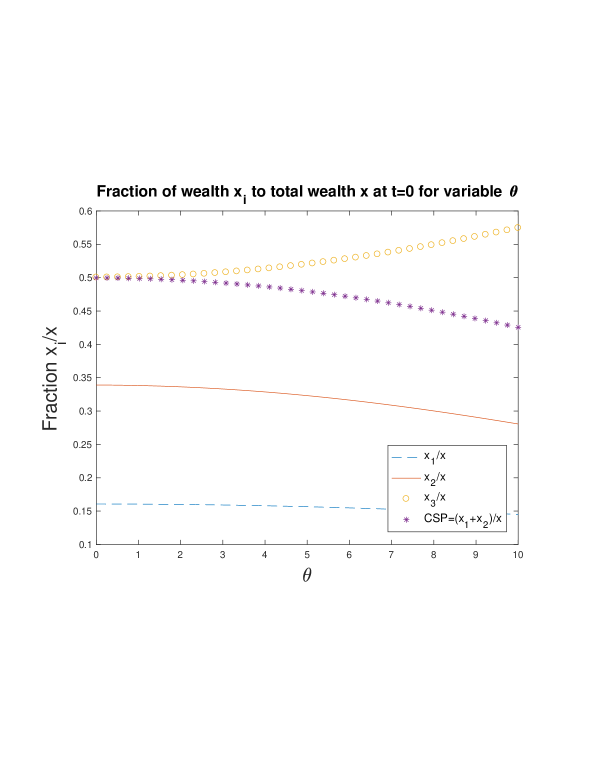
Figure 1: Fraction of initial wealth as a function of $\theta$.

Let us next explore the effect of first agent change in risk aversion on CSP. In figure 2, we vary $\gamma_{1}$ while holding $\gamma_{2}=-3,$ and $\gamma_{3}=-2.$ As expected, when agent 1 becomes more risk-averse his initial wealth allocation for financing his/her consumption increases and this will translate in an increase in CSP. By looking at figure 2 we notice that the effect of first agent change in risk aversion on CSP is considerable; a change in first agent risk aversion will cause up to $50\%$ change in CSP.

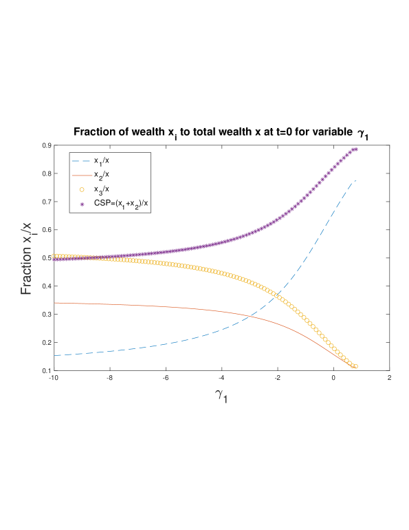
Figure 2: Fraction of initial wealth as a function of risk aversion $\gamma_{1}$, for $\gamma_{1}\leq\gamma_{3}$.

We conclude by exploring the effect of the couple change in risk aversion on CSP. In figure 3, we vary $\gamma_{3}$ while holding $\gamma_{1}=-9,$ and $\gamma_{2}=-3.$ As expected the initial wealth allocation for financing investment increases in $\gamma_{3}$ (since the couple becomes less risk averse). This in turn will make CSP decrease in $\gamma_{3}.$ By looking at figure 3 we notice that the effect of the couple change in risk aversion on CSP is considerably; a change in couple risk aversion will cause up to $70\%$ change in CSP.

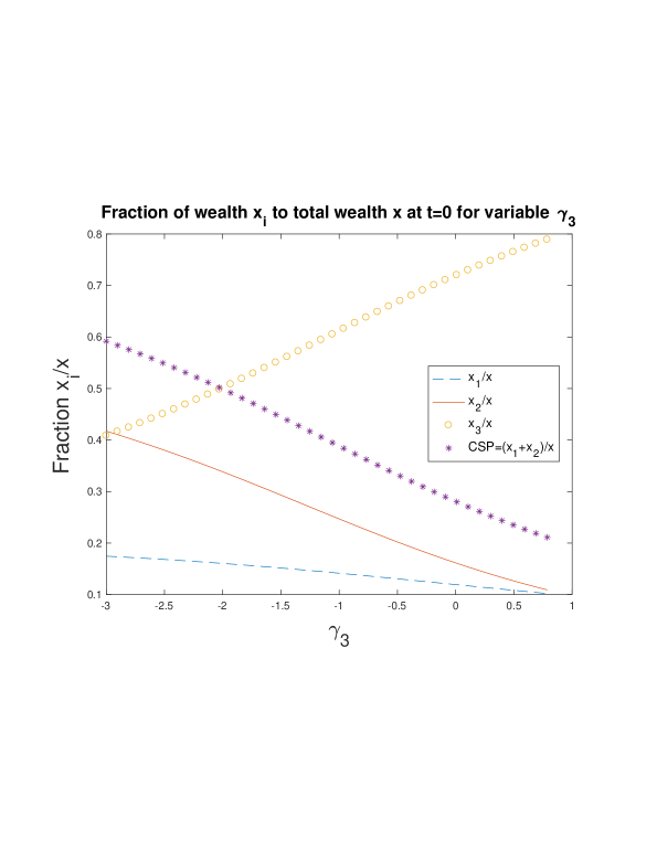
Figure 3: Fraction of initial wealth as a function of $\gamma_{3}$.

References

- [1] Martin Browning. The saving behaviour of a two-person household. scandinavian Journal of Economics, 102(2):235–251, 2000.
- [2] Martin Browning and Annamaria Lusardi. Household saving: Micro theories and micro facts. Journal of Economic literature, 34(4):1797–1855, 1996.
- [3] P Cheridito and Y. Hu. Optimal consumption and investment in incomplete markets with general constraints. Stochastics and Dynamics, 11(2):283–299, 2011.
- [4] Pierre-André Chiappori. Rational household labor supply. Econometrica: Journal of the Econometric Society, pages 63–90, 1988.
- [5] Pierre-Andre Chiappori. Collective labor supply and welfare. Journal of political Economy, 100(3):437–467, 1992.
- [6] Pierre-Andre Chiappori and Maurizio Mazzocco. Static and intertemporal household decisions. Journal of Economic Literature, 55(3):985–1045, 2017.
- [7] Ivar Ekeland, Oumar Mbodji, and Traian A Pirvu. Time-consistent portfolio management. SIAM Journal on Financial Mathematics, 3(1):1–32, 2012.
- [8] E. Fama and K. French. Permanent and temporary components of stock prices. Journal of Political Economy 96, 246 - 273, 1988.
- [9] J.M. Harrison and S.R. Pliska. Martingales and stochastic integrals in the theory of continuous trading. Stochastic processes and their applications, 11(3):215–260, 1981.
- [10] H Horst, Y. Hu, Imkeller, A Reveillac, and J. Zhang. Forward-backward systems for expected utility maximization. Stochastic Processes and their Applications, to appear, 2014.
- [11] Y. Hu, P Imkeller, and M. Müller. Utility maximization in incomplete markets. Ann. Appl. Probab., 15(3):1691–1712, 2005.
- [12] C. Huang and R. H. Litzenberger. Foundations for financial economics. 1988.
- [13] I. Karatzas, J. P. Lehoczky, and S. E. Shreve. Optimal portfolio and consumption decisions for a small investor; on a finite horizon. SIAM J. Control Optim., 25(6):1557–1586, November 1987.
- [14] I. Karatzas and S. E. Shreve. Brownian motion and stochastic calculus. Graduate Texts in Mathematics, 113, 1987.
- [15] T.S. Kim and E. Omberg. Dynamic nonmyopic portfolio behavior. Review of Financial Studies, 9(1):141–161, 1996.
- [16] Marilyn Manser and Murray Brown. Marriage and household decision-making: A bargaining analysis. International economic review, pages 31–44, 1980.
- [17] Maurizio Mazzocco. Household intertemporal behaviour: A collective characterization and a test of commitment. The Review of Economic Studies, 74(3):857–895, 2007.
- [18] D Meyer and J. Meyer. Relative risk aversion: What do we know? Journal of Risk andUncertainty, 31(3):243–262, 2005.
- [19] Salvador Ortigueira and Nawid Siassi. How important is intra-household risk sharing for savings and labor supply? Journal of Monetary Economics, 60(6):650–666, 2013.
- [20] OSFC. Evidence for mean reversion in equity prices. Office of the Superintendent of Financial Institutions of Canada, March, 2012.
- [21] J. Poterba and L.H. Summers. Mean reversion in stock prices: Evidence and implications. Journal of Financial Economics 22, 27 - 59, 1988.
- [22] P. Six. Dynamic strategies when consumption and wealth risk aversion differ. Revue Finance, 31:93–118, 2010.
- [23] J.A. Wachter. Portfolio and consumption decisions under mean-reverting returns: An exact solution for complete markets. Journal of financial and quantitative analysis, 2002.
- [24] B Wong and C. C. Heyde. On changes of measure in stochastic volatility models. Journal of Applied Mathematics and Stochastic Analysis, pages 1–13, 2006.