A Measurement-based Analysis of the
Energy Consumption of Data Center Servers

Abstract

Energy consumption is a growing issue in data centers, impacting their economic viability and their public image. In this work we empirically characterize the power and energy consumed by different types of servers. In particular, in order to understand the behavior of their energy and power consumption, we perform measurements in different servers. In each of them, we exhaustively measure the power consumed by the CPU, the disk, and the network interface under different configurations, identifying the optimal operational levels. One interesting conclusion of our study is that the curve that defines the minimal CPU power as a function of the load is neither linear nor purely convex as has been previously assumed. Moreover, we find that the efficiency of the various server components can be maximized by tuning the CPU frequency and the number of active cores as a function of the system and network load, while the block size of I/O operations should be always maximized by applications. We also show how to estimate the energy consumed by an application as a function of some simple parameters, like the CPU load, and the disk and network activity. We validate the proposed approach by accurately estimating the energy of a map-reduce computation in a Hadoop platform.

.

1 Introduction

Massive data centers are becoming common nowadays. Large companies such as Google, Yahoo!, Amazon or Microsoft have deployed large data centers, housing tens of thousands of servers, and consuming a huge amount of energy every year. According to Van Heddeghem and Lambert [8], data centers’ total energy consumption in $2012$ was about $270$ TWh, which corresponds to almost $2\%$ of the global electricity consumption, and has an approximated annual growth rate of $4.3\%$. This trend has driven researchers all over the world to focus on energy efficiency in data centers. Examples of energy saving techniques proposed during the recent years are virtualization plus consolidation and scheduling optimization [12, 17]. However, industry requirements keep increasing, and more research is necessary.

In this paper, out of all possible components of a data center, e.g., servers, routers, switches, etc., we concentrate on the characterization of servers and the energy they consume. Indeed, in order to obtain full benefit of the aforementioned energy-efficient techniques, it is crucial to have a good characterization of servers in the data center, as a function of the utilization of the server’s components. That is, it is necessary to know and understand the energy and power consumption of servers and how this changes under the different configurations. There is a large body of literature on characterizing servers’ energy and power consumption. However, the existing literature does not jointly consider phenomena like the irruption of multicore servers and dynamic voltage and frequency scaling (DVFS) [21], which are key to achieve scalability and flexibility in the architecture of a server. With these new parameters, more variables come into play in a server configuration. Learning how to deal with these new parameters and how they interact with other variables is important since this may lead to larger savings.

It has been traditionally considered that the CPU is responsible for most of the power being consumed in a server, and that this power increases linearly with the load. Although the power consumed by the CPU is significant, we believe that the power incurred by other elements of the server, like disks and NICs (Network Interface Cards) are not negligible, and have to be taken into account. Moreover, we believe that the assumption that CPU power consumption depends linearly from the load in a server may be too simplistic, especially when the server has multiple cores and may operate at multiple frequencies. In fact, even the way load is expressed has to be carefully defined (e.g., it cannot be defined as a proportion of the maximal computational capacity of the CPU, since this value changes with the operational frequency). Therefore, more complex/complete models for the power consumed by a server are necessary. In order to be consistent, these models have to be based on empirical values. However, we found that there is a lack of empirical work studying servers energy behavior.

Our work tries to partially fill this void by proposing a measurement-based characterization—which is the first of its kind—of the energy consumption of a server with DVFS and multiple cores. We evaluate here different server machines and evaluate what is the contribution to their power consumption of the CPU, hard drive disk, and network card (NIC). Our results support, for instance, our belief that more complex models than linear are required for CPU power consumption. From the measurements obtained from the servers we evaluate, we propose a holistic energy consumption characterization, that accounts for the power consumed by CPU, disk, and NIC. Our approach captures the influence of the processing frequency and the multiple cores, not only to the CPU power consumption, but also to that of disk input/output (I/O) and NIC activity.

Main results and contributions

Our main contributions are of two kinds: $(i)$ we propose a methodology for empirically characterizing the energy consumption of a server, and $(ii)$ we provide novel insights on the power and energy consumption behavior of the most relevant server’s components.

As concerns the methodology, we observe that active CPU cycles per second (ACPS) is a convenient metric of CPU load in architectures using multiple frequencies and cores. We show how to isolate the contribution to energy/power consumption due to CPU, disk I/O operations, and network activity by just measuring the total server power consumption and a few activity indicators reported by the operating system. We also show that the baseline power consumption of a server—i.e., the power consumed just because the server is on—has a strong weight on the total server consumption.

As concerns the components’ characterization, we show that, besides the baseline component, the CPU has the largest impact among all components, and its power consumption is not linear with the load. Disk I/O operations are the second highest cause of consumption, and their efficiency is strongly affected by the I/O block size used by the application. Eventually, network activity plays a minor yet not negligible role in the energy/power consumption, and the network impact scales almost linearly with the network transmission rate. All other components can be accounted for in the baseline power consumption, which is subject to minor variations under different operational conditions.

The main results of our campaign of measurements and analysis can be listed as follows:

• The CPU consumption depends on the number of active cores, the CPU frequency, and the load (in ACPS units). Our measurements confirm that the power consumption with a single active core at constant frequency can be closely approximated by a linear function of the load. However, given a CPU frequency, the power consumption is a concave function of the load and can be approximated by a low-order polynomial. The power consumption for a fixed load is, in general, minimized by using the highest number of cores and the lowest frequency at which the load can be served. However, the minimum achievable power consumption is a piecewise concave function of the load.

• The power consumed by hard disks for reading and writing depends on CPU frequency and I/O block sizes. Both reading and writing costs increase slightly with the CPU frequency. While the consumption due to reading is not affected by block size, the power consumed when writing increases with the block size. The reading efficiency (expressed in MB/J) is barely affected by the CPU frequency, while writing efficiency is a concave function of the block size since it boosts the throughput of writing until a saturation value is reached.

• The power consumption and the efficiency of the NIC, both in transmission and reception, depends on the CPU frequency, the packet size, and the transmission rate. The efficiency of data transmission increases almost linearly with the transmission rate, with steeper slopes corresponding to lower CPU frequencies. Although a linear relation between transmission rate and efficiency holds for data reception as well, small packet sizes yield higher efficiency in reception.

• Overall, we provide a holistic energy consumption model that only requires a few calibration parameters for every different server that we want to evaluate (a universal power model will be too simplistic and inaccurate). We validate our model by means of a server computing the pagerank metric of a graph in a Hadoop platform, with bulky network activity, and we found that the error due our energy estimates is below $7\%$.

2 Methodology

In this section we introduce the measurement techniques we used to characterize the power consumption of CPU activity, disk access (read and write operations), and network activity. Our measurements start characterizing the CPU power consumption, from where we obtain information about the baseline power consumption of the system. After CPU and baseline characterization, we follow with experiments for the other two components, namely, disk and network. Note that CPU and baseline measurements are of capital importance in order to evaluate the other components, because any operation run in a machine is like a puzzle with multiple pieces and we must know what is the contribution of each one of these pieces. Consider that, we are paying a cost just for having a server switched on and the operating system running on it. Similarly, every time we run a task in the system, some CPU cycles are needed in order to execute it as well as to use the component that has to perform the task. Hence, in order to understand the contribution of any component, we first need to identify the contribution of the CPU and compute the difference with respect to the aforementioned baseline.

To explore the possible parameters determining the power consumption of a server and to gain statistic consistency we run our experiments multiple times. Similarly, we run these experiments in different servers and architectures in order to validate our results and give consistency to our conclusions.

2.1 Collecting system data and fixing frequency parameters

One prerequisite for our experiments was having Linux machines due to the kind of commands and benchmarks we wanted to use and, mainly, because of the possibility of adding some kernel modules and utilities, which allows us to change CPU frequencies at will. In a Linux system, CPU activity stats are constantly logged, so we can periodically read the core frequency and the number of active and passive CPU ticks at each core. Once we have the number of ticks and the core frequency, since a tick represents a hundredth of second, cycles can be calculated as $100$ ticks/frequency.

We use active cycles per second (ACPS) instead of CPU load percentage to characterize CPU load because the latter depends on the CPU frequency used, as the higher the frequency the more the work that can be processed. Hence, a percentage of load is not comparable when different frequencies are used, while the amount of ACPS that can be processed can be considered as an absolute magnitude. In order to get and set information about the operative frequency of the system we used the cpufrequtils package. With those tools, we can monitor the CPU frequency at which the system works and assign different frequencies to the cores. However, to limit the number of possible combinations to characterize, we fix the frequency to be the same for all cores.

2.2 Baseline

The first experiment we ran in any machine was what we called the baseline experiment. The intention of this experiment is to measure the consumption of the system when it is running nothing but the OS and our own script. Similarly, we keep disks and memory slots connected but disconnect any network cable.

Our script registers the amount of active ticks consumed during time slots of $30$ seconds for each one of the different available frequencies in a machine. With this experiment we gain some insights in what is the average power consumed just by having a machine switched on in an almost idle state. Knowing this baseline will mainly help us to understand the range in which consumption varies when we run CPU experiments.

2.3 CPU

In order to evaluate the CPU power consumption we prepared a script based on the benchmark application, namely lookbusy. Note that lookbusy allows us to load one or more CPU cores with the same load.Our lookbusy-based experiment follows the next steps: we first fix the CPU frequency to the lowest possible frequency in the system; then we run lookbusy with fixed amount of load for one core during timeslots of $30$ seconds, starting with the maximum load and then decreasing the load gradually. After the last lookbusy run we measure the power consumed during an additional timeslot with no lookbusy load offered. We register the active cycles and the power used during each timeslot.

After taking these different samples for one frequency we move to the immediately higher frequency (we can list and change frequencies thanks to cpufrequtils) and repeat the previous steps. After going through all the available frequencies, we restart the whole process but increasing by one the number of active cores. We repeat this whole process until all the cores of the server are active. Note that when we change the frequency of the cores we change it in all of them, active or not, for consistency. Similarly, when we have more than one active core, the load for all the active cores will be the same.

Once explained the scheme of our experiments, we must clarify the meaning of running a timeslot with no load. Note that zero-load is clearly not possible as there is always going to be load in the system due to, e.g., the operating system. However, during the timeslot in which we do not run lookbusy, we measure the power corresponding to the operational conditions which are as close as possible to the ones of an idle system. Moreover, the decision of using timeslots of $30$ seconds is to guarantee enough, yet not excessive, time for the measurements. In fact, as we start and stop lookbusy at the beginning and end of the timeslots, we need to ignore the first and the last few seconds of measurements in each timeslot to avoid measurement noise due to power ramps and operational transitions.

The measured values of load (in ACPS) and power in each timeslot are used to obtain a least squares polynomial fittings curve. These fittings characterize the CPU power consumption for each combination of frequency and number of active cores. We will use as baseline power consumption of each one of these configurations the zero-order coefficient of the polynomial of these fittings curves.

povray performs a graphic test with a given number of cores. In our povray based experiment we will run povray for each combination of frequency and number of active cores.

As the povray task requires a constant number of cycles to be performed, this allows us to evaluate the time required to perform the same task as well as the energy spent during that execution in each one of the analyzed cases. For instance, in a machine with $10$ available frequencies and $4$ cores each execution would consist of $4\cdot 10$ povray runs.

Finally, as we had previously computed the baseline consumption we can, quite accurately, know what was the increase in the consumption due to this experiments. Furthermore, this characterization of CPU will lead us to a better understanding of the behavior of the remaining components as, when we run a read(write) operation, send (receive) data from the network,…, we are not only using each of those devices but also the CPU. Each time we execute the commands that lead to those actions, a certain amount of CPU cycles is needed to process them, then, in order to know what is the increase in the consumption due to the HDD (NIC, memory,…) we first need to subtract the consumption due to the CPU. Only then we will know what is the contribution of each one of these elements separatedly.

2.4 Disks

The power consumption of the hard drive was evaluated using $2$ different scripts (for reading and writing) based on the dd linux command. We chose dd as it allows us to read files, write files from scratch, control the size of the blocks we write (read), control the amount of blocks written (read) and force the commit of writing operations after each block in order to reduce the effect of operating system caches and memory. We combine this tool with flushing the RAM and caches after each reading experiment.

In both our scripts we perform write (read) operations for a set of different I/O block sizes and for different data volumes to be written (read). In each case we record the CPU active cycles, the total power and time consumed in each one of these operations for each combination of block size and available frequency.

Finally, we identify the contribution of the hard drive to the total power consumption by subtracting the contribution of both the baseline and the CPU consumption from the measured total power.

Disk I/O experiments shed light on the relevance of the block sizes when reading or writing as well as whether there is an influence of the frequency on these operations.

2.5 Network

In order to evaluate the contribution of the network to the power consumption of a server, we devised a set of experiments based on the iperf tool as well as on our own UPD-client-server C script. For the network loading we use a simple UDP client-server application written in C. The network load is controlled using a for-loop in the client side that increases processing and delays the packet transmission. Inside the for-loop we include a modulo operation (because some compilers are clever enough to understand if there is some work to be done inside the for-loop and if not they skip the for-loop) and every time that the modulo operation results to zero the client sends a packet to the server. Algorithm 2.5 describes the traffic control that we described earlier.

[ruled]LoadControlload, pktSize LoadControlload, pktSizetotalPkts load / (pktSize*8)
load ≤maxLoad loopController 1200 *
(1000/load) * (pktSize/1470);
k 1 totalPkts j 1 loopController j (modloopController) = 0 SendPacket();

There are several aspects that we consider relevant in order to characterize the impact of the NIC on the total power consumption of a server and that led us to choose these two tools. The first is the ability of performing tests where the computer under study acts as a server (sender) or as a client (receiver) of the communication, in order to observe its behavior when sending data or receiving it. For the sake of clarity, we will use, from now on, the terms sender, for the server injecting traffic to the network, and receiver for the server accepting traffic from the network. The second aspect consists in the ability to change several parameters that we consider relevant for this characterization, namely, the packet size and the offered load, jointly with the frequency of the system.

Our experiments consist, then, on measuring the data rate achieved, the CPU active cycles and the total power consumption of the server under study acting as sender or receiver when using different packet sizes and different rates. We run each experiment multiple times for statistical consistency.

Finally, in order to isolate the consumption from the network, we characterize with the CPU active cycles measured in the experiment the consumption due to the CPU and the baseline and subtract them from our measurements.

3 Measurements

3.1 Devices and Setup

In order to monitor and store the instantaneous power consumed by a server during the different experiments we used a Voltech PM1000+ power analyzer, which is able to measure the total instantaneous power consumed by the server under test on a per-second basis. In order to take our measurements we connected the server being measured to the power analyzer and the latter to the power supply. In the experiments where the network was not involved (CPU and disk), we unplugged the network cable from the server, which has an impact on the power consumption as the port goes idle. In the network based experiments we established an Ethernet connection between the server under study and a second machine in order to study the server behavior, both as a receiver as well as as a sender.

Table 1: Characteristics of the servers under study

Component	Servers
	Survivor	Nemesis	Erdos
CPU (# cores)	4	$4$	$64$
# freqs	8	11	$5$
Freqs List	$1.2$ GHz, 1.333 GHz, 1.467 GHz, 1.6 GHz, 1.733 GHz, 1.867 GHz, 2 GHz, $2.133\;$ GHz	1.596 GHz, 1.729 GHz, 1.862 GHz, 1.995 GHz, 2.128 GHz, 2.261 GHz, 2.394 GHz, 2.527 GHz, 2.666 GHz, 2.793 GHz, $2.794\;$ GHz	1.4 GHz, 1.6 GHz, 1.8 GHz, 2.1 GHz, $2.3\qquad$ GHz
RAM	$4$ GB	$4$ GB	$512$ GB
Disk	$2$ TB	$2+3$ TB	$2\times 146$GB
			$4\times 1$ TB
Network	$1$ Gbps	$3\times 1$ Gbps	$4\times 1$ Gbps, $2\times 10$ Gbps

We evaluated three different servers: Survivor, Nemesis, and Erdos. We will now present these servers although their main characteristics, including their sets of available CPU frequencies, can be also found in Table 1. Survivor has an Intel Xeon E5606 $4$-core processor, with $4$ GB of RAM, a $2$ TB Seagate Barracuda XT hard drive and a $1$ Gigabit Ethernet card integrated in the motherboard. Nemesis is a Dell Precision T3500 with an Intel Xeon W3530 $4$-core processor, $4$ GB of RAM, 2 hard drives (a $2$ TB Seagate Barracuda XT and a $3$ TB Seagate Barracuda), a $1$ Gigabit Ethernet card integrated in the motherboard, and a separate Ethernet card with two $1$ Gigabit ports. In this study we only evaluate the Seagate Barracuda XT disk and the integrated Ethernet card. Both Survivor and Nemesis use the Ubuntu Server edition 10.4 LTS Linux distribution. Finally, Erdos is a Dell PowerEdge R815 with 4 AMD Opteron 6276 16-core processors (i.e., 64 cores in total), $512$ GB of RAM, two $146$ GB SAS hard drives configured as a single RAID1 system (which is the “disk" analyzed here) and four $1$ TB Near-line SAS hard drives. It also includes four $1$ Gigabit and two $10$ Gigabit ports. Erdos is a high-end server and uses Linux Debian 7 Wheezy.

3.2 Baseline and CPU

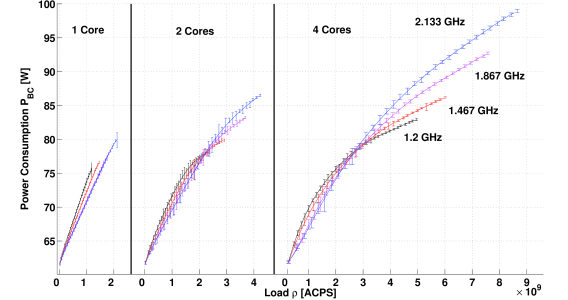
(a) Survivor

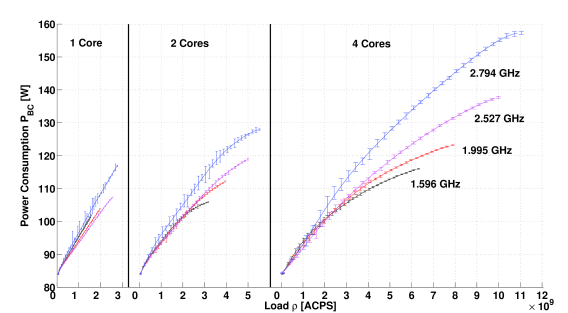
(b) Nemesis

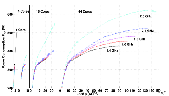
(c) Erdos

Figure 1: Power consumption of $3$ servers (Survivor, Nemesis, and Erdos) for baseline and CPU characterization experiments.

As mentioned in the previous section, for each server we have measured the power it consumes without disk accesses nor network traffic. We assume that the power consumption observed is the sum of the baseline consumption plus the power consumed by the CPU. We have obtained samples of the power consumed under different configurations that vary in the number of active cores used, the frequency at which the CPU operates (all cores operate at the same frequency), and the load of the active cores (all active cores are equally loaded). The list of available and tested CPU frequencies and cores can be found in Table 1. We tune the total load $\rho$ by using lookbusy, as described in the previous section. Each experiment lasts $30$ s and it is repeated $10$ times. Results are summarized in terms of average and standard deviation. Specifically, in the figures reported in this section, the power consumption for each tested configuration is depicted by means of a vertical segment centered on the average power consumption measured, and with segment size equal to two times the standard deviation of the samples.

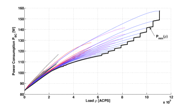
(a) Minimal power.

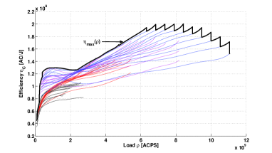
(b) Maximal efficiency.

Figure 2: CPU performance bounds of Nemesis.

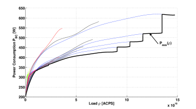
(a) Minimal power.

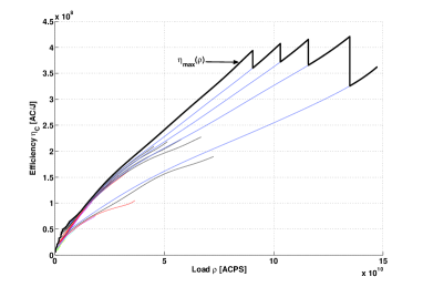
(b) Maximal efficiency.

Figure 3: CPU performance bounds of Erdos.

The results of these experiments for each of the $3$ servers are presented in Figure 1 (the measurements for some frequencies and some number of cores are omitted for clarity). Here, for each configuration of number of active cores, frequency, and load in ACPS, the mean and standard deviation of all the experiments with that configuration are presented. Also the least squares polynomial fitting curve for the samples is shown for each number of cores and frequency. The curves shown are for polynomials of degree $7$, but we observed that using a degree $3$ polynomial instead does not reduce drastically the quality of the fit (e.g., the relative average error of the fitting increases from $0.7\%$ with $7$-th degree polynomials to $1.5\%$ with degree equal to $3$ for Erdos, while it remains practically stable and below $0.7\%$ for Nemesis). In general, we can use an expression like the following to characterize the CPU power consumption:

$$\centering P_{BC}(\rho)=\sum_{k=0}^{n}\alpha_{k}\rho^{k},\quad n\leq 7,\@add@centering$$ (1)

where $P_{BC}$ includes both the baseline power consumption of the servers and the power consumed by the CPU, and $\rho$ is the load expressed in active cycles per second. Therefore, coefficient $\alpha_{0}$ in Eq. 1 represents the consumption of the system when the CPU activity tends to $0$, and we can thereby interpret $\alpha_{0}$ as the baseline power consumption of the system. Note that the polynomial fitting, and hence the baseline power consumption $\alpha_{0}$, depends on the particular combination of number of cores and frequency adopted. However, for sake of readability, we do not explicitly account for such a dependency in the notation.

A first observation of the fitting curves for each particular server in Figure 1 reveals that the power for near-zero load is almost the same in curves (e.g., for Nemesis this value is between 84 and 85 W). Observe that it is impossible to run an experiment in which the load of the CPU is actually zero to obtain the baseline power consumption of a server. However, all the fitting curves converge to a similar value for $\rho\rightarrow 0$, which can be assumed to represent the baseline power consumption.

A second observation is that for one core the curves grow linearly with the load. However, as soon as two or more cores are used, the curves are clearly concave, which implies that for a fixed frequency the efficiency grows with the load (we will discuss later the efficiency in terms of number of active cycles per energy unit).

A third observation is that frequency does not significantly impact the power consumption when the load is low. In contrast, at high load, the consumption clearly increases with the CPU frequency. More precisely, the power consumption grows superlinearly with the frequency, for a fixed load and number of cores. This is particularly evident in the curves characterizing Erdos, which is the most powerful among our servers.

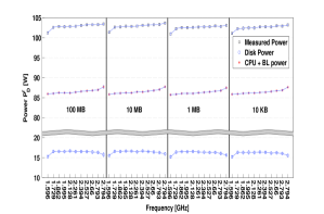
(a) Power consumption during reading (Nemesis).

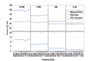
(b) Power consumption during writing (Nemesis).

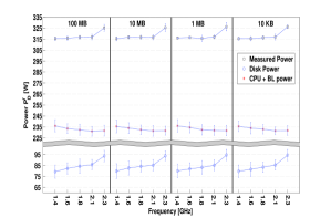
(c) Power consumption during reading (Erdos).

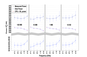
(d) Power consumption during writing (Erdos).

Figure 4: Instantaneous power consumption for a reading/writing operations. Results are presented for every frequency and for $4$ different block sizes for each one of our servers.

From the previous figures it emerges that the power consumption due to CPU and baseline can be minimized by selecting the right number of active cores and a suitable CPU frequency. Similarly, we can expect that the energy efficiency, defined as number of active cycles per energy unit, can be maximized by tuning the same operational parameters. We graphically represent the impact of operation parameters on power consumption and energy efficiency in Figures 2 and 3 respectively for Nemesis and Erdos (results for Survivor are similar to the ones shown for Nemesis and are omitted). In particular, Figures 2(a) and 3(a) report all possible fitting curves for the power consumption measurements, plus a curve marking the lowest achievable power consumption at a given load. We name such a curve “minimal power curve” $P_{\min}(\rho)$, and we observe that $(i)$ it only depends on the load $\rho$, and $(ii)$ it is a piecewise concave function, which makes it suitable to formulate power optimization problems. Finally, to evaluate the energy efficiency of the CPU, we report in Figures 2(b) and 3(b) the number of active cycles per energy unit obtained from our measurements respectively for Nemesis and Erdos. We compute the power due to active cycles as the power $P_{BC}-\alpha_{0}$, i.e., by subtracting the baseline consumption from $P_{BC}$, and we obtain the efficiency $\eta_{C}$ by dividing the load (in active cycles per second) by the power due to active cycles:

$$\eta_{C}=\frac{\rho}{P_{BC}(\rho)-\alpha_{0}}.$$ (2)

Also in this case we show the curve that maximizes the efficiency at a given load, which we name “Maximal efficiency curve” $\eta_{\max}(\rho)$. Interestingly, we observe that $(i)$ $\eta_{\max}(\rho)$ presents multiple local maxima, $(ii)$ for a given configuration of frequency and number of active cores, the efficiency is maximized at the highest achievable load, $(iii)$ all local maxima corresponds to the use of all available active cores, but $(iv)$ the absolute maximum is not achieved neither at the highest CPU frequency nor at the lowest.

3.3 Disks

We now characterize the power and energy consumption of disk I/O operations. During the experiments, we continuously commit either read or write operations, while keeping the CPU load $\rho$ as low as possible (i.e., we disconnect the network and we do not run other tasks). Still, the power measurements obtained during the disk experiments contain both the power used by the disk and power due to CPU and baseline. Indeed, Figure 4 shows, for each experiment, the total measured power $P_{t}$, the power $P_{BC}$ computed according to Eq. 1 at the load $\rho$ measured during the experiment, and the power due to disk operations, computed as:

$$P_{D}^{x}=P_{t}-P_{BC}(\rho),\quad x\in\{r,w\},$$ (3)

where superscripts $r$ and $w$ refer to reading and writing operations, respectively. We test sequentially all the available frequencies for each server (see Table 1), and I/O block sizes ranging from $10$ KB to $100$ MB. Figure 4 shows average and standard deviation of the measures over $10$ experiment repetitions. Results for Survivor are omitted since they are like Nemesis’ results. Indeed, Survivor and Nemesis have similar disks and file systems, while Erdos is equipped with SAS disks with RAID. In all cases shown in the figure, the disk power is small but not negligible with respect to the baseline consumption. Furthermore, we can observe that the two servers presented behave differently. Indeed, while the power consumption due to writing is affected both by the block size $B$ for both machines, we observe that Nemesis’ disk writing power $P_{D}^{w}$ is not affected by the CPU frequency, while Erdos’ results show an increase with the frequency. Moreover, the results obtained with Erdos are affected by a substantial amount of variability in the measurements, which we believe is due to the caching operations enforced by the RAID mechanism in Erdos.

Similarly to what was described for the CPU, we now comment on the energy efficiencies $\eta_{D}^{r}$ and $\eta_{D}^{w}$ of disk reading and writing operations. Figure 5 reports efficiency as a function of the I/O block size, and shows one line per each CPU frequency. The efficiency is computed by subtracting the baseline power from the total power, and by measuring the volume $V$ of data read or written in an interval $T$:

$$\eta_{D}^{x}=\frac{V}{P_{D}^{x}T},\quad x\in\{r,w\}.$$ (4)

We can observe that results are similar for all the servers. Specifically, the efficiency of reading is almost constant at any frequency and for each block size, while writing is more efficient with large block sizes. We also observe that the efficiency changes very little with the adopted CPU frequency. Another observation is that the efficiency saturates to a disk-dependent asymptotic value, which is due to the mechanical constraints of the disk (e.g., due to the non-negligible seek time, the number of read/write operations per second is limited). In addition, although not visible in the figure due to the log-scale adopted, $\eta_{D}^{w}$ is a concave function of the block size $B$.

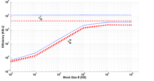
Figure 5: Disk reading and writing efficiencies for Erdos (red dotted lines) and Nemesis (blue solid lines).

3.4 Network

The last server component that we characterize via measurements is the network card. Similarly to the cases described previously, we run experiments in which only the operating system and our test scripts are active. In this case, we run a script to either transmit or receive UDP packets over a gigabit Ethernet connection and count the system active cycles $\rho$. We measure the total power consumption $P_{t}$ during the experiment, so that the power due to network activity can be then estimated as follows:

$$P_{N}^{x}=P_{t}-P_{BC}(\rho),\quad x\in\{s,r\},$$ (5)

where superscripts $s$ and $r$ refer to the sender and the receiver cases, respectively.

In the experiments, we sequentially test all the available frequencies for each server (see Table 1), and fix the packet size $S$ and the UDP transmission rate within the achievable set of rates (which depends on the packet size, e.g., $<950$ Mbps for $1470$-B packets). We report results for the network energy in terms of efficiencies $\eta_{N}^{s}$ and $\eta_{N}^{r}$ (volume of data transferred per unit of energy). These efficiencies are computed as follows:

$$\eta_{N}^{x}=\frac{R}{P_{N}^{x}},\quad x\in\{s,r\},$$ (6)

where $R$ is the transmission rate during the experiment.

Table 2: Polynomial fitting for network efficiency. The table reports empirically evaluated coefficients for Eq. 7 (coefficients $\beta_{1}$ are expressed in $W^{-1}$ while coefficients $\beta_{2}$ are in $W^{-1}\cdot\textit{bps}^{-1}$).

	RECEIVER
	Survivor					Nemesis
		$1.2$ GHz	$1.6$ GHz	$1.867$ GHz	$2.133$ GHz		$1.596$ GHz	$1.995$ GHz	$2.394$ GHz	$2.794$ GHz
$\beta_{1}$	64 B	1.751e-2	1.314e-2	1.268e-2	1.254e-2	64 B	1.491e-2	1.410e-2	1.330e-2	1.227e-2
$\beta_{2}]$		1.904e-5	2.160e-5	1.395e-5	1.031e-5
$\beta_{1}$	500 B	1.736e-2	1.386e-2	1.144e-2	9.962e-3	500 B	1.565e-2	1.234e-2	1.107e-2	1.074e-2
$\beta_{2}$		2.627e-6	1.595e-6	2.836e-6	3.541e-6
$\beta_{1}$	1000 B	1.560e-2	1.296e-2	1.132e-2	1.029e-2	1000 B	1.170e-2	9.451e-3	7.712e-3	7.448e-3
$\beta_{2}$		3.155e-6	1.736e-6	1.080e-6	1.208e-6
$\beta_{1}$	1470 B	1.497e-2	1.216e-2	1.073e-2	2.684e-2	1470 B	1.072e-2	8.849e-3	8.207e-3	8.040e-3
$\beta_{2}$		3.231e-6	4.006e-6	3.533e-6	-4.746e-6
	SENDER
	Survivor					Nemesis
		$1.2$ GHz	$1.6$ GHz	$1.867$ GHz	$2.133$ GHz		$1.596$ GHz	$1.995$ GHz	$2.394$ GHz	$2.794$ GHz
$\beta_{1}$	64 B	2.239e-2	1.802e-2	1.582e-2	1.462e-2	64 B	1.642e-2	1.313e-2	1.029e-2	8.625e-3
$\beta_{1}$	500 B	1.742e-2	1.576e-2	1.429e-2	2.205e-2	500 B	1.599e-2	1.130e-2	1.234e-2	1.014e-2
$\beta_{1}$	1000 B	1.784e-2	1.634e-2	1.454e-2	2.230e-2	1000 B	1.767e-2	1.781e-2	1.824e-2	1.179e-2
$\beta_{1}$	1470 B	1.801e-2	1.620e-2	1.461e-2	2.369e-2	1470 B	1.703e-2	1.863e-2	1.279e-2	1.134e-2

Figure 6 shows the network efficiencies of Nemesis and Survivor averaged over $3$ samples per transmission rate $R$. For sake of readability, the figure only shows results for the extreme value used for the packet size, and for three CPU frequencies: the lowest, the highest, and an intermediate frequency in the set of available frequencies reported in Table 1 for Nemesis and Survivor. The figure also reports the polynomial fitting curves for efficiency, which we found to be at most of second order. Since the efficiency is represented in terms of network activity only, in the fitting we force the zero-order coefficient of the polynomials to be $0$. Therefore, we can use the following expression to characterize the network efficiencies of our servers:

$$\eta_{N}^{x}=\beta_{1}R+\beta_{2}R^{2},\quad x\in\{s,r\},$$ (7)

where the $\beta_{i}$ coefficients are computed by minimizing the least square error of the fitting. Table 2 gives the fitting coefficients for sending and receiving efficiencies for the cases shown in Figure 6 and for other tested configurations.

From both the figure and the table, we can observe that efficiencies are almost linear or slightly superlinear with the transfer rate, e.g., the receiving efficiency of Survivor exhibits an evident quadratic behavior. Indeed, our measurements show that the network power consumption is independent from the throughput, which is a well known result for legacy Ethernet devices. In fact, the NICs of our servers are not equipped with power saving features like, e.g., the recently standardized IEEE 802.3az [9].

In all cases, the efficiency is strongly affected by the selected CPU frequency. Moreover, efficiency is also affected by packet size, although the impact of packet size changes from server to server, e.g., Survivor sending efficiency is only slightly affected by it.

Another observation is that, depending on the packet size and frequency used, sending can be more energy efficient than receiving at a given transmission rate, and using the highest CPU frequency is never the most efficient solution. Note also that the efficiency decreases with the packet size, although this effect is particularly evident at the receiver side, while it only slightly impacts the efficiency of the packet sender. However, network activity also causes non-negligible CPU activity, as shown in Figure 7 for a few experiment configurations for Nemesis. Overall, the lowest CPU frequency yields the lowest total power consumption during network activity periods.

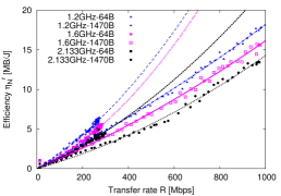
(a) Receiver network efficiency (Survivor).

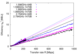
(b) Receiver network efficiency (Nemesis).

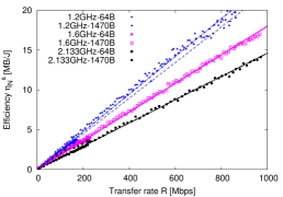
(c) Sender network efficiency (Survivor).

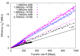
(d) Sender network efficiency (Nemesis).

Figure 6: Network efficiencies for different frequencies and $64$-B and $1470$-B packets.

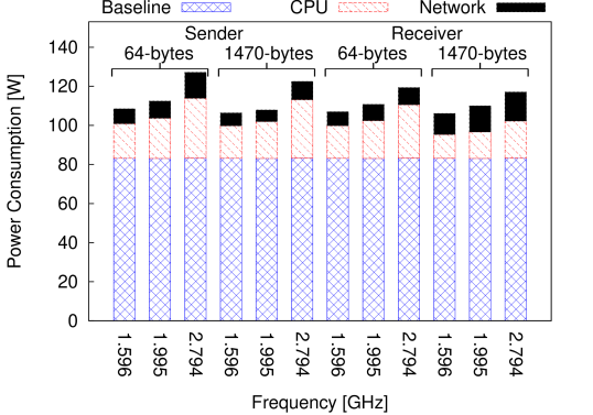
Figure 7: Power consumption with network activity for Nemesis ($64$-B experiments were run with a transmission rate $R=150$ Mbps, while $R=400$ Mbps for the experiments with $1470$-B packets).

4 Estimating Energy Consumption

While the results presented in the previous sections are useful to understand the power consumption pattern of CPU, disk and network, we believe that a much more important use of these results is to estimate the energy consumption of applications. In this section we describe how this could be done from simple data about the application, and validate the proposed process by estimating the energy consumed by map-reduce Hadoop computations.

4.1 Energy Estimation Hypothesis

The process we propose to estimate the energy consumed $E_{app}$ by an application has as basic assumption that this energy is essentially the sum of the baseline energy $E_{B}$ (the baseline power times the duration of the execution), the energy consumed by the CPU $E_{C}$, the energy consumed by the disk $E_{D}$, and the energy consumed by the network interface $E_{N}$. I.e.,

$$E_{app}=E_{B}+E_{C}+E_{D}+E_{N}.$$ (8)

Hence, the process of estimating $E_{app}$ is reduced to estimating these four terms. In order to estimate the first two terms, we need to know the total number of active cycles that the application will execute, $C_{app}$, and the load $\rho_{app}$ (in ACPS) that the execution will incur in the CPU. From this, the total running time $T_{app}$ can be computed as

$$T_{app}=C_{app}/\rho_{app}.$$ (9)

Then, once the number of cores and the frequency that will be used have been defined, it is also possible to estimate the baseline power plus CPU power, $P_{BC}$, from the fitting curves of Figure 1. This allows to estimate the sum of the first two terms of Eq. 8 as

$$E_{B}+E_{C}=P_{BC}T_{app}=P_{BC}C_{app}/\rho_{app}.$$ (10)

The energy consumed by the disk is simply the energy consumed while reading and writing, i.e., $E_{D}=E_{D}^{r}+E_{D}^{w}$. To estimate these latter values, the block size to be used has to be decided, from which we can obtain an estimate of the efficiency of reading, $\eta_{D}^{r}$, and writing, $\eta_{D}^{w}$ (see Figure 5). These, combined with the total volume of data read and written by the application, denoted as $V_{D}^{r}$ and $V_{D}^{w}$ respectively, allow to obtain the estimate energy as

$$E_{D}=\frac{V_{D}^{r}}{\eta_{D}^{r}}+\frac{V_{D}^{w}}{\eta_{D}^{w}}.$$ (11)

Finally, to estimate $E_{N}$, the transfer rate $R$ and packet size $S$ has to be chosen, which combined with the frequency used, yield sending and receiving efficiencies $\eta_{N}^{s}$ and $\eta_{N}^{r}$ (see Figure 6). Then, if the total volume of data to be sent and received is $V_{N}^{s}$ and $V_{N}^{r}$, respectively,

$$E_{N}=\frac{V_{N}^{s}}{\eta_{N}^{s}}+\frac{V_{N}^{r}}{\eta_{N}^{r}}.$$ (12)

All is left to do to obtain the estimate $E_{app}$ is to add up the values obtained in Equations 10, 11, and 12.

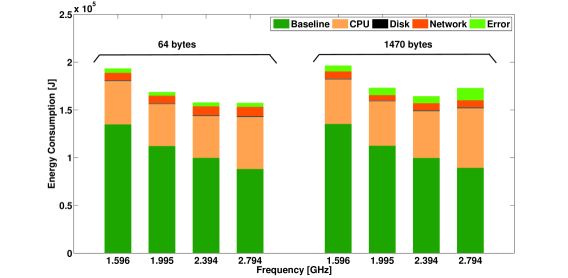
(a) Sender side.

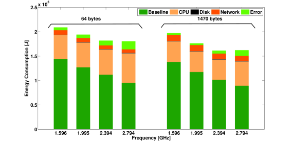
(b) Receiver side.

Figure 8: Comparison of the real versus estimated energy consumption values.

4.2 Empirical Validation

We test now the process and hypothesis presented above for the estimation of the energy consumed by an application. For that, we have chosen to execute in Nemesis a map-reduce Hadoop application that computes several iterations of the pagerank algorithm on an Erdos-Renyi random (directed) graph with 1 million nodes and average degree 5. Since the pagerank application does not use the network, while it is running we execute another process generating network traffic. This provides a richer experiment.

An execution of the pagerank application has three phases: preprocessing, map-reduce, and postprocessing. On its side, the map-reduce phase is a sequence of several homogeneous iterations of the pagerank algorithm. For simplicity, we only estimate the energy consumed during the map-reduce phase of the pagerank algorithm. In our experiments we run in Nemesis one instance of the pagerank application with $10$ iterations in its map-reduce phase for each one of the $11$ available frequencies. We run this experiment $4$ times, each with different characteristics of the network traffic generated in parallel. In particular, we run experiments with Nemesis behaving as a sender and as a receiving, and using packets of 64 and 1470 bytes. Instead of estimating the energy for the whole sequence of $10$ iterations, it is simpler to estimate the energy for every iteration separately. Then, for each iteration $i$ we can register the total active cycles executed $C_{app}^{i}$, the time consumed $T_{app}^{i}$, and the volume of data read and written, $V_{D}^{r,i}$ and $V_{D}^{w,i}$, respectively, and the transfer rate $R$ (the same for all iterations: $150$ Mbps for experiments with $64$-B packets and $400$ Mbps for experiments with $1470$-B packets).

Unfortunately, we cannot measure the instantaneous CPU load. Instead, we assume that the CPU load is the same during the execution for a given frequency and network configuration. Hence we estimate it as $\rho_{app}^{i}=C_{app}^{i}/T_{app}^{i}$. Then, from this value we obtain the estimate of the instantaneous power $P_{BC}^{i}$ using the fitting curves as described above. Finally, using Eq. 10 we compute the estimate $E_{B}^{i}+E_{C}^{i}$.

In order to estimate the energy consumed by the disk operations, we use the fact that Hadoop uses a block size of $64$ MB. This allows us to estimate the reading and writing efficiencies, $\eta_{D}^{r,i}$ and $\eta_{D}^{w,i}$ (see Figure 5). Combining these values with the measured volume of data read and written ($V_{D}^{r,i}$ and $V_{D}^{w,i}$) as described in Eq. 11, we obtain $E_{D}^{i}$.

Finally, to estimate the network consumption in one iteration with Nemesis sending traffic (resp., receiving traffic), the sending efficiency $\eta_{N}^{s},$ (resp., receiving efficiency $\eta_{N}^{r}$) is obtained from the transfer rate $R$, and the frequency and packet size used (see Figure 6). The amount of data sent (reps., received) is obtained as the product of the rate $R$ and the time $T_{app}^{i}$. Then, the energy of the network is obtained using Eq. 12.

Once we have computed the energy due to the different components in iteration $i$, the total energy $E_{app}^{i}$ is obtained by adding them. Adding these values for the $10$ iterations of an experiment we obtain the estimate $E_{app}$. The (approximate) total real energy $\hat{E}_{app}^{i}$ consumed by iteration $i$ is computed by obtaining the average value of the power samples we registered with our power analyzer during the iteration, and multiplying it by $T_{app}$. Again, the total energy consumed by the experiment are obtained as $\hat{E}_{app}=\sum_{i=1}^{10}\hat{E}_{app}^{i}$. The estimation error for each experiment is then computed as $\hat{E}_{app}-E_{app}$.

We show the results obtained for four selected frequencies (the results for the rest are similar) in Figure 8(a), for the sender cases, and Figure 8(b) for the receiving cases. Each figure includes the results for the two packet sizes used. As can be seen, the error is very small (always below $7\%$ of the total energy), being a bit more relevant in the case of the highest frequency.

5 Discussion

We discuss now some of the implications of our results. We start with consolidation. It has been typically assumed that the best way of doing consolidation is to fill servers as much as possible, to reduce the total number of servers being used, hence proposing bin-packing based solutions [3, 15, 20] and not necessarily having frequency into account. However, the results presented in Figures 2(b) and 3(b) show that the highest frequency is not the most efficient one, and this has been found to be true for two different architectures (Intel and AMD). This implies that, by running servers at the optimal amount of load, and the right frequency, a considerable amount of energy could be saved.

A second relevant aspect is the baseline consumption of servers. The results presented for all $3$ servers show that their baselines are within a $30$-$50\%$ of the maximum consumption. Then, it is straightforward that more effort is to be done for reducing baseline consumption. For instance, a solution could consist in switching off cores in real time, not just disabling them, or in introducing very fast transitions between active and lower energy states, i.e., to achieve real suspension in idle state.

Finally, we refer to the CPU load associated to disk and network activity. It can be observed in Figure 4 that disks do not incur much CPU overhead. In fact, the power consumed by CPU plus baseline does not change much across the experiments. Instead, the energy consumed by CPU due to network operations is even larger than the energy consumed by the NIC (see Figure 7). Some works [7] have already pointed out that the way the packets are handled by the protocol stack is not energy efficient. Our results reinforce this feeling and point out that building a more efficient protocol stack would certainly reduce the amount of energy consumed due to the network.

6 Related Work

Various works that try to estimate the energy/power consumption of servers exist in the literature.

Many of them are already outdated since they do not take into consideration the DVFS technology, such as [13], [14] , [5], [19], [11] and [2]. In all papers the authors propose models to estimate the energy consumption due to CPU, disk, memory, electromechanical parts (e.g. fans and optical drives) and board components ( e.g support chipsets, voltage regulators, connectors, interface devices etc.). Conversely, they do not consider the effect of different frequencies or the effect of the network or both. In [14] Liu et al propose iops/s per Joule( I/O operations per second) as their metric and they observe the impact of using different combination based on the number of cores and the amount of offered memory. In [5] the MANTIS model for estimating the power consumption of a server has a similar to our calibration methodology but the effect of multiple frequencies does not appear. The metrics used are the CPU utilization and the I/O request rates to the hard drives. Vasan et al [19] measure the total power consumption of a server without stressing the server using some benchmark but they measure the current load of the different parts of the server, i.e. memory, network, CPU, disk operations. Their model is very simplistic and is not compared with the real measurements to check if it corresponds to the actual power consumption.

this is for virtual machines if we need In [11] In 

Another category of works study the effect of DVFS, [16, le2010dynamic, ge2010powerpack, howard201148]. We mention [16] because it is one of the first works evaluating the performance of DVFS is a strongARM SA-1100 processor. The authors show the results of three power management techniques, frequency scaling, clock throttling and dynamic voltage and frequency scaling. The authors show the superlinear behavior of the CPU power consumption when DVFS is used. In their results they show that a server that has both idle and high activity behavior throughout the day, there is critical frequency that below that it is inefficient because the task will take longer due to lower performance and in addition going idle becomes cheaper below that critical voltage point. In [le2010dynamic] the authors experience a power saving of 34% using the CPU with DVFS enabled. The benchmark used introduces idle periods and the gain appears because of those periods. They do not perform full characterization under any amount of load and the frequency of operation is randomly selected by the CPU. Ge et al. [ge2010powerpack] propose PowerPack, a framework that includes a set of toolkits to profile the power consumption of severs, composed of hardware and software components. The authors provide data from measurements on the CPU, on the disk on the memory on the CPU fan and on the network. They have isolated the power consumed by each of those components. Furthermore, they run their benchmarks for different frequencies and different amount of cores and they keep track of the power consumption. The drawback of their measurements is that they compare the variation of the power consumption over time and since the benchmark is used as a blackbox we cannot conclude the most efficient point of operation. Although their measurements show that reducing the frequency leads to lesser power consumption while adding some extra delay to finish the task. In [howard201148] the authors study among others the impact of DVFS in an experimental 48-core processor. They show that using higher frequency and voltage the processor consumes much more power when operates at full load conditions. Even in the lowest possible voltage the power consumed by the memory controllers of the processor dominates the power consumed by the cores where the latter corresponds only to 21% of the total power consumed by the processor.

In [inoue2011power] Inoue et all. model the power consumption of both HDD and SSD hard disks. They do not take into consideration other data sizes than 1024 bytes and they do not perform any measurements regarding the different frequencies of the CPU (which may affect the power consumption of C, CR and CW processes).

Various metrics have been used to evaluate the energy efficiency of servers. In [kumar2003single] $IPS^{2}/Watt$ (million instructions committed per second per Watt) is used. In [21] MIPJ (millions of instructions per Joule) is proposed.

There is a large body of work in the field of modeling server power consumption and its components, both theoretical and empirical. The consumption of servers has been assumed as linear e.g., by Wang et al. [20], Mishra et al. [15] or Beloglazov et al. [3], who assumed models where consumption depended mainly on CPU and linearly on its utilization, proposing bin-packing-like algorithms to reduce power consumption. Other works like the ones from Andrews et al. [1] or Irani et al. [10] proposed non-linear models, claiming that energy could be saved by running processes at the lowest possible speed.

Moving to the empirical field, we first classify works in two different groups, those who consider the effect of frequency on their analysis and those who do not consider it. We start with those not considering frequency. In this category we find articles proposing models where server components follow a linear behavior like [11, 14, 19] or more complex ones, like in  [2, 5, 13]. In  [14], Liu et al. propose a simple linear model and evaluate different hardware configurations and types of workloads by varying the number of available cores, the available memory, and considering also the contribution of other components such as disks. Vasan et al. [19] monitored multiple servers on a datacenter as well as the power consumption of several of the internal elements of a server. However, they considered that the behavior of this server could be approximated by a model based only on CPU utilization. Similarly, Krishnan et al. [11] explored the feasibility of lightweight virtual machine power metering methods and examined the contribution of some of the elements that consume power in a server like CPU, memory and disks. Their model depends linearly on each of these components. In [5], Economou et al. proposed a non-intrusive method for modeling full-system power consumption by stressing its components with different workloads. Their resulting model is also linear on the utilization of its components. Finally, Lewis et al. [13] and Basmasjian et al. [2] presented much more complex models which, apart from the contribution of different components of the server, considered extra parameters like temperature and cache misses as well as multiple cores. In particular, Lewis et al. [13] reported also an extensive study on the behavior of reading and writing operations in hard disk and solid state drives. In contrast, we show that linear models are not accurate and we complement the existing studies by showing the effect of different block sizes and frequencies, e.g., on network and individual read or write operations.

Now we move to the works which also considered frequency in their analysis. Miyoshi et al. [16] analyzed the runtime effects of frequency scaling on power and energy. Brihi et al. [4] presented an exhaustive study of DVFS using a cpufrequtils as we do. Main differences with our work were that they studied four different power management policies under DVFS and centered their study on the relationship between CPU utilization and power consumption. However, they also present interesting results about disk consumption that match partially our results, showing a flat consumption in reading operations and variations in the writing ones that they attribute to the size of the files being written. Although it was not the main objective of their work, Raghavendra et al. [18] performed a per-frequency and core CPU power characterization of two different blade servers. However, they claimed that CPU power depends linearly on its utilization. The main difference with our analysis is that we consider that the load supported by a server increases with the number of active cores and, hence, this load should not be represented in percentage. Gandhi et al. [6] published a preliminary analysis of power consumption versus frequency, based on DVFS and DFS and gave some intuition about the non-linearity of this relation. However, our analysis is more complete as we present a per-component analysis as well as enter into deeper details on the power versus frequency analysis.

7 Conclusions

In this work we have reported our measurement-based characterization of energy and power consumption in a server. We have exhaustively measured the power consumed by CPU, disk, and NIC under different configurations, identifying the optimal operational levels, which usually do not correspond to the static system configurations commonly adopted. We found that, besides the baseline component, which does not changes significantly with the operational parameters, the CPU has the largest impact on energy consumption among all the three components. We observe that CPU consumption is neither linear nor concave with the load. Disk I/O is the second larger contributor to power consumption, although performance changes sensibly with the I/O block size used by the applications. Finally, the NIC activity is responsible for a small but not negligible fraction of power consumption, which scales almost linearly with the network transmission rate. In general, most of the energy/power performance figures do not scale linearly with the utilization, in contrast to what is commonly assumed in the literature. We have then shown how to predict and optimize the energy consumed by an application via a concrete example using network activity plus pagerank computation in Hadoop. Our model achieves very accurate energy estimates, within $7\%$ or less from the measured total power consumption.

References

- [1] Andrews, M., Antonakopoulos, S., and Zhang, L. Minimum-cost network design with (dis)economies of scale. In IEEE FOCS (2010), pp. 585–592.
- [2] Basmadjian, R., Ali, N., Niedermeier, F., de Meer, H., and Giuliani, G. A methodology to predict the power consumption of servers in data centres. In ACM e-Energy (2011), pp. 1–10.
- [3] Beloglazov, A., Abawajy, J., and Buyya, R. Energy-aware resource allocation heuristics for efficient management of data centers for cloud computing. Future Generation Computer Systems 28, 5 (2012), 755–768.
- [4] Brihi, A., and Dargie, W. Dynamic voltage and frequency scaling in multimedia servers. In IEEE AINA (2013).
- [5] Economou, D., Rivoire, S., Kozyrakis, C., and Ranganathan, P. Full-system power analysis and modeling for server environments. In Proceedings of Workshop on Modeling, Benchmarking, and Simulation (2006), pp. 70–77.
- [6] Gandhi, A., Harchol-Balter, M., Das, R., and Lefurgy, C. Optimal power allocation in server farms. In ACM SIGMETRICS (2009), pp. 157–168.
- [7] Garcia-Saavedra, A., Serrano, P., Banchs, A., and Bianchi, G. Energy consumption anatomy of 802.11 devices and its implication on modeling and design. In ACM CoNEXT (2012), pp. 169–180.
- [8] Heddeghem, W. V., Lambert, S., Lannoo, B., Colle, D., Pickavet, M., and Demeester, P. Trends in worldwide ICT electricity consumption from 2007 to 2012. Computer Communications (Submitted).
- [9] IEEE Std. 802.3az. Energy Efficient Ethernet, 2010.
- [10] Irani, S., Shukla, S., and Gupta, R. Algorithms for power savings. ACM TALG 3, 4 (2007), 41.
- [11] Krishnan, B., Amur, H., Gavrilovska, A., and Schwan, K. VM power metering: feasibility and challenges. ACM SIGMETRICS Performance Evaluation Review 38, 3 (2011), 56–60.
- [12] Kusic, D., Kephart, J. O., Hanson, J. E., Kandasamy, N., and Jiang, G. Power and performance management of virtualized computing environments via lookahead control. Cluster computing 12, 1 (2009), 1–15.
- [13] Lewis, A. W., Ghosh, S., and Tzeng, N.-F. Run-time energy consumption estimation based on workload in server systems. HotPower’08 (2008), 17–21.
- [14] Liu, C., Huang, J., Cao, Q., Wan, S., and Xie, C. Evaluating energy and performance for server-class hardware configurations. In IEEE NAS (2011), pp. 339–347.
- [15] Mishra, M., and Sahoo, A. On theory of vm placement: Anomalies in existing methodologies and their mitigation using a novel vector based approach. In IEEE CLOUD (2011), pp. 275–282.
- [16] Miyoshi, A., Lefurgy, C., Van Hensbergen, E., Rajamony, R., and Rajkumar, R. Critical power slope: understanding the runtime effects of frequency scaling. In ACM ICS’02 (2002), pp. 35–44.
- [17] Moore, J. D., Chase, J. S., Ranganathan, P., and Sharma, R. K. Making scheduling “cool”: Temperature-aware workload placement in data centers. In USENIX annual technical conference, General Track (2005), pp. 61–75.
- [18] Raghavendra, R., Ranganathan, P., Talwar, V., Wang, Z., and Zhu, X. No power struggles: Coordinated multi-level power management for the data center. In ACM SIGARCH Computer Architecture News (2008), vol. 36, ACM, pp. 48–59.
- [19] Vasan, A., Sivasubramaniam, A., Shimpi, V., Sivabalan, T., and Subbiah, R. Worth their Watts? - An empirical study of datacenter servers. In IEEE HPCA (2010), pp. 1–10.
- [20] Wang, M., Meng, X., and Zhang, L. Consolidating virtual machines with dynamic bandwidth demand in data centers. In IEEE INFOCOM (2011), pp. 71–75.
- [21] Weiser, M., Welch, B., Demers, A., and Shenker, S. Scheduling for reduced CPU energy. In Mobile Computing. Springer, 1996, pp. 449–471.