Mode density and frequency extraction in $\delta$ Scuti star HD 50844

Abstract

We consider the high mode density reported in the $\delta$ Scuti star HD 50844 observed by CoRoT. Using simulations, we find that extracting frequencies down to a given false alarm probability by means of successive prewhitening leads to a gross over-estimate of the number of frequencies in a star. This is due to blending of the peaks in the periodogram due to the finite duration of the time series. Prewhitening is equivalent to adding a frequency to the data which is carefully chosen to interfere destructively with a given frequency in the data. Since the frequency extracted from a blended peak is not quite correct, the interference is not destructive with the result that many additional fictitious frequencies are added to the data. In data with very high signal-to-noise, such as the CoRoT data, these spurious frequencies are highly significant. Continuous prewhitening thus causes a cascade of spurious frequencies which leads to a much larger estimate of the mode density than is actually the case. The results reported for HD 50844 are consistent with this effect. Direct comparison of the power in the raw periodogram in this star with that in $\delta$ Scuti stars observed by Kepler shows that HD 50844 has a typical mode density.

1 Introduction

The $\delta$ Scuti class of variables are dwarfs or giants with spectral types between A2 and F5. They lie on an extension of the Cepheid instability strip with periods in the range 0.02–0.3 d. Most of the pulsational driving in these stars is by the $\kappa$ mechanism in the HeII partial ionization zone. A large number of $\delta$ Sct stars have been identified in photometric time series data from the Kepler spacecraft. A study of these stars by Balona & Dziembowski (2011) has revealed that even in the center of the instability strip, no more than half the stars pulsate as $\delta$ Sct variables. This is a surprising finding; the reason for damping of pulsations in constant stars in the instability strip is presently not known.

Prior to the MOST, CoRoT and Kepler space missions, it was thought that the frequency spectra in $\delta$ Sct stars may become very dense as the detection threshold is lowered. The reason is that modes of high degree, $l$, which are not seen from the ground because of the low amplitudes due to cancellation effects, should be easily seen at the precision level attained for these space missions (Balona & Dziembowski, 1999). Indeed, this expectation appears to have been fulfilled in CoRoT observations of HD 50844 (Poretti et al., 2009). This star appears to have a very high mode density over the whole frequency range, indicating that modes of relatively high $l$ are seen. However, in a study of Kepler $\delta$ Sct stars, Balona & Dziembowski (2011) find that, in general, the mode density is quite moderate and that HD 50844 is probably an exception.

In order to study mode density, one needs to be sure that frequencies are correctly extracted from the data. This is not an issue for the high amplitude peaks in the periodogram, but since the number of modes is expected to increase with decreasing amplitude, one needs to estimate the probability that a given peak is due to noise (the false-alarm probability). The significance level of a frequency can be estimated easily only for the case of an equally-spaced time series, when the Lomb-Scargle criterion can be used (Scargle, 1982). When the sampled times are not uniformly spaced, the problem is intractable and can only be solved by numerical means (Frescura et al., 2008). Ground-based data are seldom equally spaced and the “four-sigma” rule is often used to estimate the significance level (Breger et al., 1993). This rule states that a peak is deemed significant if its amplitude exceeds the background noise level of the periodogram by a factor of four. This is a purely empirical rule with no statistical foundation, but does seem to be reasonable in many cases (Kuschnig et al., 1997; Koen, 2010). The CoRoT data are uniformly spaced and it is therefore important to apply the correct statistics.

For a time series of duration, $t$, the width of a peak in the power spectrum is inversely proportional to $t$. Thus for a time series of a given duration, there is a maximum limit on the number of peaks per frequency interval that can be measured. Since the mode density is expected to increase with decreasing amplitude, blending of peaks due to the finite frequency resolution becomes very important. Thus the number of frequencies that can be extracted, and hence the mode density, depends not only on a correct estimation of the false alarm probability, but also on effects related to the finite frequency resolution. These effects have not been taken into account in estimates of mode density by Poretti et al. (2009) and Balona & Dziembowski (2011).

From the above considerations, it is clear that one needs to carefully reconsider the question of significance in frequency extraction for CoRoT and Kepler data and, in particular, the importance of frequency resolution and close frequencies. In this paper we use simulations at various mode densities to determine the effect of mode density on frequency extraction. We also compare results obtained with the Lomb-Scargle false alarm probability (FAP) criterion with those calculated using the four-sigma rule. It turns out that neither of these criteria are useful if the number of modes increases with decreasing amplitude. Finally, we compare the amplitude density in the periodogram of HD 50844 with those of Kepler $\delta$ Scuti stars.

2 The data and noise properties

The CoRoT observations of HD 50844 consist of $n=155827$ white light data points obtained between HJD 2452590.0684 and HJD 2452647.7817 (57.7 d) with a cadence of 30 s. The time series is almost uninterrupted, except for data taken at the southern magnetic anomaly and some other points which were rejected because they were clearly anomalous.

We first of all need to understand the noise properties of these data. One way to do this is to select stars which appear to be constant, or vary the least. The noise level in the periodogram of such a star may be used to calibrate the noise level in any other star in a purely empirical way.

The definition of what is meant by the noise level in the periodogram needs to be clarified. In visual estimates of the noise level, this is generally taken as the height of the majority of peaks. The peaks in the periodogram may be likened to blades of grass on a lawn and the mean height of the peaks may be called the “grass” level. This loose definition has been placed on a firmer footing by Balona (2011) who defined $\sigma_{G}=2.5\sigma$, where $\sigma$ is the median height of the periodogram peaks in a region free of signals. In the four-sigma rule, a peak with amplitude $A$ may be considered significant if $A>4\sigma_{G}$. One may also define the mean background noise level as just the average of the power or the amplitude. Since the background noise level typically increases towards low frequencies, and since the backgound is often difficult to estimate in crowded regions of the spectrum, the exact meaning of “mean background level” is often not clear.

It can be shown that the mean amplitude, $A$, of the periodogram of pure white noise with variance $\sigma_{0}$ is given by $A=2\sigma_{0}/\sqrt{n}$, where $n$ is the number of points in the time series (see Kendall (1976)). From the high-frequency tail of the periodogram of HD 50844 we find $A=0.0035$ mmag which gives $\sigma_{0}=0.691$ mmag. Cast in terms of apparent magnitude, $V$, and duration of the time series, $\Delta t$, the noise level in the periodogram can be written as

$$\log\sigma_{G}=a+\frac{1}{5}V-\frac{1}{2}\log\Delta t,$$

where $a$ is a constant. By fitting 175 of the least variable stars in the A–F range in the Kepler data, Balona (2011) found

$$\log\sigma_{G}=-0.93+0.21V-0.47\log\Delta t,$$

where $\sigma_{G}$ is measured in ppm and $\Delta t$ in days, confirming the expected relationship.

In the case of the CoRoT data, we do not have access to a large number of constant or nearly constant A–F stars for a completely independent estimate of the noise level. However, we do have data for HD 292790, also measured by Poretti et al. (2009). This star is variable at low frequencies, but the noise level is well defined at the higher frequencies relevant for $\delta$ Sct stars. The magnitude of HD 292790 is $V=9.48$ and the time-series duration $\Delta t=54.66$ d. For the $\delta$ Scuti star HD 50844, $V=9.09$ and $\Delta t=57.70$ d. Fig. 1 shows the periodograms for these two stars. Fig. 2 shows an expanded region to show the noise levels.

The periodogram of HD 292790 can be understood in terms of rotation of a spotted star with frequency $f=0.4386$ d^-1 (Poretti et al., 2009). The periodogram contains a signal at 13.9668 d^-1 and its harmonics which is the orbital frequency of the satellite. For this star we estimate $\sigma_{G}=5$ ppm, which allows us to determine the constant $a$ in the above equation. We obtain

$$\log\sigma_{G}=-0.33+0.2V-0.5\log\Delta t,$$

which means that Kepler data are about four times more precise than CoRoT data. This formula gives $\sigma_{G}=4.0$ ppm for HD 50844, which is indeed the noise level of the high frequency tail in Fig. 2. Thus, according to the four sigma rule, we may assume that for HD 50844 only frequencies with amplitudes exceeding approximately 16 ppm are likely to be real.

The spectral window of the CoRoT data for HD 50844 is shown in Fig. 3. The FWHM of the central peak is about 0.02 d^-1, which means that frequencies separated by less than about 0.01 d^-1 are not likely to be resolved.

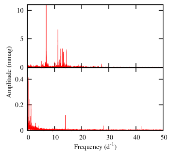
Figure 1: Periodograms of HD 50844 (top) and HD 292790 (bottom). The estimated noise level for HD 50844 is $\sigma_{G}=4.0$ ppm while for HD 292790 it is $\sigma_{G}=5.0$ ppm (see Fig. 2 for an expanded view).

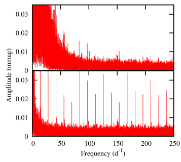
Figure 2: Periodograms of HD 50844 (top) and HD 292790 (bottom) with expanded amplitude scale to show the noise level.

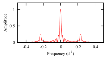
Figure 3: Spectral window of the HD 50844 CoRoT data.

3 Tests of significance

Although the four-sigma test of significance is widely used because it is simple to apply, it is by no means a rigorous test. For example, Koen (2010) finds that the actual significance levels corresponding to the four sigma limit may vary by orders of magnitude, depending on the exact data configuration. He finds that the number and time spacing of the observations have little influence on the significance levels. On the other hand, the total duration of the time series, the frequency range that is searched and previous prewhitening of the data greatly affect the significance level of the four sigma rule. In particular, prewhitening removes too much power at the given frequency, hence the estimated mean noise level is lower than it should be, decreasing the false alarm probability. This means that repeated application of the rule on successively prewhitened data will tend to assign significance to peaks which are probably noise. Koen (2010) also find that the four sigma rule, when applied to a single frequency peak, is likely to underestimate its significance. In other words, there are peaks of lower amplitude which are significant, but which are considered to be noise by the four-sigma rule.

More precise significance tests for periodograms have been discussed by, among others, Scargle (1982); Horne & Baliunas (1986); Koen (1990) and Schwarzenberg-Czerny (1998). Somewhat different methods are discussed by Reegen (2007); Reegen et al. (2008) and Baluev (2008). An excellent discussion of the problem is presented by Frescura et al. (2008). The problem is clearly a very difficult one for data which is not uniformly sampled. For uniformly-sampled data Scargle’s significance test (Scargle, 1982) is easy to calculate and gives the false-alarm probability of a periodogram peak given the power level and the noise variance of the data. Since the CoRoT and Kepler data are equally sampled, except for occasional small gaps, it is clear that this test is to be preferred to the four-sigma rule.

For equally-spaced data, Scargle (1982) shows that the false-alarm probability (FAP), $P(z)$, of a peak with power $z$ is given by

$$P(z)=1-\left\{1-\exp(-z/\sigma^{2}_{0})\right\}^{N_{i}},$$

where $\sigma^{2}_{0}$ is the noise variance of the data and $N_{i}$ is the number of independent frequencies. We call this the Lomb-Scargle significance criterion. It should be noted that in some references the power is normalized by the noise variance, while in others it is not. We use the un-normalized definition. This relationship can be inverted to give the power for any FAP,

$$z=-\sigma^{2}_{0}\ln\left\{1-\left(1-P(z)\right)^{1/N_{i}}\right\}.$$

The number of independent frequencies is well defined only for equally-spaced data and is given by $N_{i}=n/2$, where $n$ is the number of data points (Frescura et al., 2008). Astronomers usually prefer the periodogram to be a function of amplitude rather than power. For our definition of power, $z$, the amplitude is given by $A=2\sqrt{z/n}$. Given a certain FAP, $P_{A}$, one may then calculate an amplitude, $A_{A}$, which corresponds to this probability,

$$A_{A}=2\sqrt{-\frac{\sigma^{2}_{0}}{n}\ln\left\{1-\left(1-P_{A}\right)^{1/N_{i}}\right\}}.$$

For CoRoT observations of HD 50844, we find $A_{A}=0.014$ mmag for $P_{A}=0.01$ and $A_{A}=0.015$ mmag for $P_{A}=0.001$. The four-sigma rule suggests that only amplitudes above 0.016 mmag are significant, which is certainly true, but is very stringent and corresponds to a FAP of less than 0.001, whereas a FAP of $P_{A}=0.01$ is often sufficient.

4 Simulations

Before we apply the Lomb-Scargle criterion to the CoRoT data of HD 50844, it is important to test it on synthetic data. These tests take the actual times of CoRoT observations of this star to generate a time series comprising of many sinusoidal variations with randomly generated frequencies, amplitudes and phases. The simulations consist of uniformly distributed frequencies in the range 0–30 d^-1, which is roughly the frequency range of pulsations in HD 50844. In $\delta$ Sct stars, the number of modes increases sharply with decreasing amplitude. To roughly mimic this, the amplitudes in our simulations are exponentially distributed. A noise error with a Gaussian distribution and standard deviation of 0.500 mmag was added to each point of the synthetic time series. This leads to a mean periodogram height of 0.0025 mmag or a grass noise level $\sigma_{G}=0.006$ mmag, roughly similar to that found in HD 50844. The aim of these simulations is to determine the effect of mode density on frequency extraction and to test the reliability of these frequencies in data with a high signal-to-noise (S/N) ratio. We also wish to investigate the efficiency of the four-sigma rule and the Lomb-Scargle significance criterion.

The time series was analyzed using the Lomb periodogram and the algorithm described by Press & Rybicki (1989) for fast implementation. The peak of maximum amplitude is located and its frequency measured by fitting a quadratic to points around maximum amplitude. This frequency, together with up to 20 previous frequencies, is used in a simultaneous least-squares Fourier fit to the data.Once the limit of 20 frequencies has been reached, the original time series is replaced by the prewhitened time series and the process repeated until the peak of highest amplitude is no longer significant.

We start with the sparsest frequency set of 30 frequencies. In this case we are able to extract 65 frequencies for which FAP $>$ 0.01 (or 47 frequencies using the four-sigma limit) even though the simulated data has only 30 frequencies. Of these frequencies, the first 28 of highest amplitude match the known frequencies. The two missing frequencies do appear, but are far down on the list since they have very low amplitudes. The question that needs to be asked is where do the additional 35 frequencies which have significant amplitudes come from?

Fig. 4 shows the periodogram in a specific frequency region and also a schematic periodogram of the same region which shows that the large peak actually consists of two unresolved closely-spaced frequencies. These frequencies and amplitudes are $f_{1}=19.3458$ d^-1, $A_{1}=7.118$ mmag, $f_{2}=19.3300$ d^-1, $A_{2}=0.574$ mmag. The figure also shows a schematic periodogram of the extracted frequencies. Instead of extracting just a single frequency, the code finds numerous, roughly equally-spaced frequency components of relatively high amplitudes. A third frequency at $f_{3}=19.4475$ d^-1, $A_{3}=1.855$ mmag also shows fictitious components.

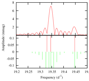
Figure 4: Schematic periodogram of known frequency components (with positive amplitudes) and extracted components (negative amplitudes) in a simulation.

The origin of these fictitious components are easy to understand. They come about because the extracted frequency of the unresolved peak is 19.3465 d^-1, which differs from the true frequency. Even though the difference is only 0.0007 d^-1, the prewhitened data still contains significant signal because the amplitude of the unresolved peak is so high. Prewhitening, in fact, is equivalent to adding a fictional signal to the data. When the prewhitening frequency and amplitude is sufficiently close to the true values, both are removed through destructive interference. If the prewhitening frequencies and amplitudes not quite correct, what remains is a sequence of equally-spaced frequencies of diminishing amplitude (an interference pattern). If the frequency of interest has a low amplitude, the residual interference pattern may be below the noise level, which is nearly always the case in ground-based observations. Space data have such high signal-to-noise ratio that the amplitudes of the residual interference pattern is well above the noise level. Thus far more frequencies are extracted than actually exist. Provided that the S/N level is sufficiently high, successive frequency extraction will lead to an ever increasing number of frequencies at low amplitudes which do not actually exist.

Table 1: Results of frequency extraction using the Lomb periodogram on simulated data. Random frequencies uniformly distributed in the range 0–30 d^-1 and random amplitudes exponentially distributed in the range 0–10 mmag were used. $N_{0}$ is the number of generated frequencies, $N$ is the number of these frequencies with amplitudes above the FAP = 0.01 threshold. $N_{\rm ex}$ is the number of extracted frequencies with FAP $<$ 0.01 using the Lomb-Scargle periodogram. The frequencies extracted using the four-sigma criterion is given by $N_{4}$. The two last columns give the numbers of significant frequencies using non-linear optimization. $L_{\rm ex}$ refers to the numbers using the Lomb-Scargle FAP and $L_{4}$ to the four-sigma criterion.

$N_{0}$	$N$	$N_{\rm ex}$	$N_{4}$	$L_{\rm ex}$	$L_{4}$
30	30	65	47	30	29
50	50	137	87	57	54
100	98	220	150	132	112
200	198	537	350	402	320
300	298	879	585	729	596
500	493	1611	1141	1439	1197
700	693	2101	1545	1976	1687
1000	998	3711	2215	2566	2283
2000	1982	3405	2805	3108	2797
3000	2969	3599	2968	3488	3187

Results of simulations using an increasing density of frequencies are shown in Table 1. We note that the four-sigma criterion is more stringent than the Lomb-Scargle FAP criterion, though it is clear that these criteria are irrelevant in identifying the true frequencies. Note also that the number of extracted frequencies increases only slowly for $N>1000$. The reason for this is due to the finite resolution imposed by the limited duration of the time series.

There are two problems that come to light. The first problem consists in unavoidable errors in blended frequencies with high amplitudes, resulting in a cascade of low-amplitude (but highly significant) fictitious frequencies. The second problem is one of frequency resolution which increases the number of blended frequencies and compounds the problem. It might be possible to recognize close frequencies using nonlinear optimization. To test this possibility we used the Levenberg-Marquard algorithm in combination with the Lomb periodogram to optimize the frequencies, grouping closely-spaced frequencies in a simultaneous optimization scheme. Results are shown in Table 1. While nonlinear optimization gives much better results for low mode densities, it still fails badly as the density increases.

Another symptom which arises from continuous prewhitening of data with very high S/N is the development of a plateau in the periodogram consisting of a very large number of blended peaks of almost equal amplitude. An example of this can be seen in the simulations arising from the simulation with $N_{0}=1000$ frequencies. Such a plateau occurs in other simulations, but is most prominent in those with a high mode density. The development of a plateau can be seen in Fig. 3 of Poretti et al. (2009).

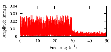
Figure 5: Periodogram of simulated data with 1000 actual frequencies after prewhitening by 2000 frequencies showing the characteristic plateau.

From these simulations we conclude that one should be very careful in extracting frequencies with small amplitudes in stars with very high S/N data containing several high-amplitude peaks. In particular, no trust should be placed in the very large number of frequencies which results from successive prewhitening in such stars. This is undoubtedly the case in HD 50844.

5 Amplitude distribution

The simulations described above show that the effect of finite frequency resolution is very important. In fact, it is likely to be of far greater importance well before the amplitude threshold appropriate to a given false alarm probability. A question that is directly relevant to estimation of the mode density is the distribution of amplitudes. In order to estimate the mode density for the lowest detectable amplitudes, one needs to calculate the amplitude distribution, i.e., the number of modes within a given amplitude range. From the results of the previous section, it is clear that repeated prewhitening will lead to an ever increasing number of false modes for low amplitudes. In this section we investigate the amplitude distribution using simulations.

For this purpose, we generated a number of time series with random frequencies uniformly distributed in the frequency range 0–30 d^-1 with uniformly distributed amplitudes in the amplitude range 0–10 mmag. This differs from the analysis in the previous section where we used an approximately exponential amplitude distribution. A uniform amplitude distribution is not expected in $\delta$ Sct stars, but it allows the known and extracted amplitude distributions to be more easily compared.

Table 2 shows the number of simulated frequencies and the number of extracted frequencies using the Lomb periodogram. We did not attempt to apply non-linear optimization of the frequencies, since this does not resolve the frequency resolution problem discussed in the previous section. Note that the number of extracted frequencies is much larger than the number of real frequencies. This is not surprising because, in general, the amplitudes in this simulation are much larger than in the exponential distribution which increases the cascading effect that arises when frequencies are unresolved.

Table 2: Results of frequency extraction using the Lomb periodogram on simulated data with uniform amplitude distribution. $N_{0}$ is the total number of simulated frequencies and $N$ is the number of simulated frequencies with amplitudes above the FAP = 0.01 threshold. $N_{\rm ex}$ is the number of extracted frequencies with FAP $<$ 0.01 using the Lomb-Scargle periodogram.

$N_{0}$	$N$	$N_{\rm ex}$
30	30	105
50	50	238
100	99	490
200	199	1226
300	299	1833
500	499	2684
700	699	3217
1000	998	3711
2000	1998	3711
3000	2996	5212

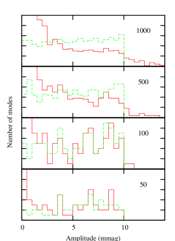
Figure 6: Distribution of amplitudes extracted from the Lomb periodogram for a selection of simulated data. The solid histogram shows the relative number of extracted frequencies as a function of amplitude (mmags). The dashed histogram is the true distribution. The panels are labeled according to the total number of known frequencies.

Table 3: Significant frequencies and amplitudes in HD 50844. The frequency $f$ is in d^-1, the amplitude $A$ in mmillimags and the phase $\phi$ in radians. This is a fit to $A\cos(2\pi f(t-t_{0})+\phi)$ with $t_{0}=2590.0000$. The second and third columns list mode identifications from spectroscopy, $(l,m)$, and radial velocity amplitudes, $A_{\rm RV}$ (km s^-1) from Poretti et al. (2009).

Term	(l,m)	$A_{\rm RV}$	$f$ (d-1)	$A$ (mmag)	$\phi$ (rad)
$f_{1}$	(0,0)	0.72	$6.92527\pm 0.00007$	$16.73\pm 0.01$	$0.575\pm 0.001$
$f_{2}$	(3,1)	0.39	$11.21672\pm 0.00008$	$6.76\pm 0.01$	$1.559\pm 0.001$
$f_{3}$	(5,1)		$11.25803\pm 0.00010$	$4.37\pm 0.01$	$0.773\pm 0.002$
$f_{4}$	(3,3)	0.52	$12.84848\pm 0.00010$	$3.55\pm 0.01$	$-2.281\pm 0.002$
$f_{5}$		0.45	$12.23840\pm 0.00009$	$3.53\pm 0.01$	$-0.010\pm 0.002$
$f_{6}$	(4,3)		$14.44681\pm 0.00008$	$3.08\pm 0.01$	$1.986\pm 0.003$
$f_{7}$	(3,2)		$13.27339\pm 0.00008$	$2.87\pm 0.01$	$-2.871\pm 0.003$
$f_{8}$	(5,3)	0.11	$13.35871\pm 0.00008$	$2.51\pm 0.01$	$1.803\pm 0.003$
$f_{9}$	(11,7)	0.05	$11.75098\pm 0.00010$	$1.58\pm 0.01$	$1.585\pm 0.005$
$f_{10}$	(2,-2)	0.08	$5.26680\pm 0.00011$	$1.24\pm 0.01$	$1.362\pm 0.007$
$f_{11}$		0.20	$14.46124\pm 0.00011$	$1.24\pm 0.01$	$0.071\pm 0.007$
$f_{12}$	(4,2)	0.10	$14.43221\pm 0.00011$	$1.08\pm 0.01$	$-2.167\pm 0.008$
$f_{13}$		0.10	$9.95266\pm 0.00011$	$1.02\pm 0.01$	$2.798\pm 0.008$
			$0.00497\pm 0.00011$	$1.26\pm 0.04$	$-2.483\pm 0.029$
$f_{14}$			$11.98370\pm 0.00011$	$0.94\pm 0.01$	$1.148\pm 0.009$
$f_{15}$			$6.55652\pm 0.00011$	$0.82\pm 0.01$	$2.895\pm 0.010$
$f_{17}$			$13.56876\pm 0.00011$	$0.85\pm 0.01$	$-3.090\pm 0.010$
$f_{16}$			$7.40484\pm 0.00011$	$0.85\pm 0.01$	$1.412\pm 0.010$
$f_{18}$	(5,0)		$10.26038\pm 0.00011$	$0.79\pm 0.01$	$-0.864\pm 0.010$
$f_{19}$		0.08	$5.78209\pm 0.00011$	$0.74\pm 0.01$	$-1.964\pm 0.011$
			$11.70934\pm 0.00012$	$0.69\pm 0.01$	$-1.332\pm 0.012$
$f_{20}$			$6.62851\pm 0.00012$	$0.71\pm 0.01$	$1.919\pm 0.012$
			$12.12271\pm 0.00012$	$0.70\pm 0.01$	$1.160\pm 0.012$
			$7.63511\pm 0.00012$	$0.66\pm 0.01$	$2.999\pm 0.013$
			$27.29546\pm 0.00012$	$0.66\pm 0.01$	$2.046\pm 0.013$
$f_{22}$	(3,1)		$14.47801\pm 0.00011$	$0.68\pm 0.01$	$1.201\pm 0.013$
			$14.23452\pm 0.00011$	$0.56\pm 0.01$	$2.125\pm 0.015$
$f_{27}$	(4,-2)		$5.67451\pm 0.00012$	$0.61\pm 0.01$	$-1.642\pm 0.014$
$2f_{1}$			$13.84992\pm 0.00012$	$0.59\pm 0.01$	$-2.488\pm 0.014$
			$4.66075\pm 0.00012$	$0.53\pm 0.01$	$0.390\pm 0.016$
			$1.28065\pm 0.00012$	$0.51\pm 0.01$	$3.041\pm 0.016$
$f_{30}$	-	0.08	$5.41839\pm 0.00012$	$0.53\pm 0.01$	$-2.480\pm 0.016$
$f_{32}$	(5,-2)		$5.49082\pm 0.00012$	$0.51\pm 0.01$	$-0.946\pm 0.016$
			$3.48107\pm 0.00012$	$0.47\pm 0.01$	$0.403\pm 0.018$
			$11.33797\pm 0.00012$	$0.48\pm 0.01$	$-0.782\pm 0.017$
			$1.17976\pm 0.00012$	$0.46\pm 0.01$	$-2.041\pm 0.018$
$f_{44}$	(6,4)		$14.60065\pm 0.00012$	$0.46\pm 0.01$	$0.842\pm 0.018$
			$14.26363\pm 0.00012$	$0.46\pm 0.01$	$0.472\pm 0.018$
			$18.72302\pm 0.00012$	$0.45\pm 0.01$	$1.073\pm 0.019$
			$7.25400\pm 0.00012$	$0.44\pm 0.01$	$2.297\pm 0.019$
			$10.62982\pm 0.00012$	$0.43\pm 0.01$	$-1.538\pm 0.019$
			$14.06179\pm 0.00012$	$0.42\pm 0.01$	$2.927\pm 0.020$
			$15.75242\pm 0.00012$	$0.42\pm 0.01$	$-0.870\pm 0.020$
$f_{43}$	(4,-2)	0.12	$5.04317\pm 0.00012$	$0.42\pm 0.01$	$-1.560\pm 0.020$
			$0.32135\pm 0.00012$	$0.42\pm 0.01$	$-0.776\pm 0.020$
			$13.06176\pm 0.00013$	$0.40\pm 0.01$	$3.040\pm 0.021$
$f_{50}$	(12,10)		$15.22420\pm 0.00012$	$0.39\pm 0.01$	$-2.349\pm 0.021$
$f_{46}$	(14,12)		$19.75031\pm 0.00012$	$0.39\pm 0.01$	$-0.179\pm 0.021$
			$1.23137\pm 0.00013$	$0.38\pm 0.01$	$-1.064\pm 0.022$
			$3.38306\pm 0.00013$	$0.37\pm 0.01$	$2.196\pm 0.023$
			$0.93230\pm 0.00013$	$0.37\pm 0.01$	$0.115\pm 0.023$
$f_{51}$	(8,5)	0.08	$11.64339\pm 0.00013$	$0.36\pm 0.01$	$1.352\pm 0.023$
			$2.22293\pm 0.00013$	$0.35\pm 0.01$	$-2.960\pm 0.024$
			$3.79566\pm 0.00013$	$0.34\pm 0.01$	$-0.829\pm 0.024$
			$3.57994\pm 0.00013$	$0.33\pm 0.01$	$-0.908\pm 0.025$
			$6.57856\pm 0.00013$	$0.35\pm 0.01$	$1.095\pm 0.024$
			$15.56830\pm 0.00013$	$0.33\pm 0.01$	$2.248\pm 0.025$
			$2.85138\pm 0.00013$	$0.32\pm 0.01$	$-1.230\pm 0.026$
			$8.56364\pm 0.00013$	$0.31\pm 0.01$	$1.316\pm 0.027$

In Fig.6 we show the distribution of amplitudes for four selected simulations. In all cases, the true distribution is flat (uniform amplitude distribution) and extends from 0–30 d^-1. The amplitude distributions derived from the extracted frequencies are very different and always show a large number of low-amplitude frequencies (out of scale in the Figure). In addition, there is considerable spillage to high amplitudes due to two or more frequencies which are unresolved. The larger the number of frequencies the greater the number of frequencies at very low and very high amplitudes.

It is clear that high mode density leads to a grossly distorted amplitude distribution obtained by successive prewhitening. In fact, numerical experiments show that if successive prewhitening is performed until the false alarm probability of the highest peak reaches a reasonable level ($P_{A}=0.01or0.001$), the resulting amplitude distribution is practically the same, independently of the actual distribution that is chosen for the simulation. The distribution is dominated by the low-amplitude peaks which are mostly false peaks arising from unresolved frequencies.

6 Avoiding prewhitening

Given the problems associated with continuous prewhitening, it is clear that another method of extracting frequencies is desirable for data with very high S/N. One possibility is simply to locate the peaks in the periodogram of the raw (i.e. non-prewhitened) data. This has to be done with care and in combination with prewhitening of the most dominant peaks because much of the structure in the periodogram is a result of the window function.

7 Frequencies in HD 50844

If we apply the Lomb-Scargle criterion to the 30-s cadence data of HD 50844 we find that there are about 1800 frequencies with amplitudes in excess of 0.014 mmag ($P_{A}=0.01$) and 1700 frequencies in excess of 0.015 mmag ($P_{A}=0.001$), mostly within the range 0–30 d^-1. This is equivalent to 60 frequencies per d^-1 which is at the limit of frequency resolution. As we have seen, these numbers are likely to be considerably larger than actually present in the star.

In Table 3 we list the frequencies of highest amplitude. Since all these frequencies have quite large amplitudes, there is no danger of them being fictitious. Our frequencies and amplitudes agree very well with those of Poretti et al. (2009) and we have adopted the same numbering scheme for the frequencies. There are very few combination frequencies; we find $f_{10}=4f_{1}-2f_{2}$ and $f_{12}=2f_{4}-f_{3}$, but these are most probably coincidences. The harmonic $2f_{1}$ is clearly visible.

8 Comparison with Kepler $\delta$ Scuti stars

One question that is of interest is whether HD 50844 has a higher mode density than other $\delta$ Scuti stars. We cannot really answer this question because it is not possible to extract frequencies below a certain threshold level. Also, we have seen that the finite time resolution and the prewhitening technique provide severe limitations on the frequencies that can be reliably extracted. What can be answered is whether the amplitude density in the periodogram is larger than in other $\delta$ Scuti stars. To do this we need to compare the amplitude density in HD 50844 with those of other stars.

The Kepler data provide by far the most homogeneous sample of light curves of $\delta$ Sct stars. Nearly all $\delta$ Sct stars observed by Kepler were discovered in the data from Quarters 0,1 and 2 which are in the public domain. However, for most of these stars the length of the time series is about 30 d. Since frequency resolution is important for determining mode density, we need to ensure that the length of the time series for each star is the same. We decided to truncate the time series of all the Kepler stars to 25 d in order to obtain the largest sample of $\delta$ Scuti stars. Also, we limit the data to stars observed with short cadence (exposure times of about 60 s). While considerably more Kepler $\delta$ Sct stars have been observed with long cadence (exposure time about 30 min), these cannot be used because the highest frequency that can be detected is only about 24 d^-1, whereas most $\delta$ Sct stars still have modes with frequencies as high as 50 d^-1.

There are 357 $\delta$ Scuti stars observed in short-cadence mode in the Kepler database. Since all these stars were observed for the same length of time, we can use the area of the periodogram above a certain amplitude level as proportional to the number of modes with amplitudes higher than this level. Fig. 7 shows this plot for the Kepler $\delta$ Sct stars. The top panel shows the plot for HD 50844; the star is clearly not exceptional in this regard.

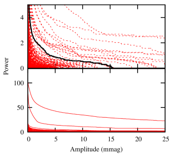
Figure 7: Relative amplitude density as a function of amplitude for Kepler $\delta$ Scuti stars. The top panel shows the same plot expanded to show HD 50844 (thick line).

9 Conclusion

Using simulations, we show that it is not possible to extract frequencies reliably down to the expected noise level using successive prewhitening. The reason is due to unresolved peaks in the periodogram which become more numerous as the amplitude decreases. Such unresolved peaks lead to a multitude of erroneous frequencies. Prewhitening by a frequency which differs from the true frequency by a significant amount leaves many frequency residuals of lower amplitude. In the high S/N data from space missions, these spurious residual frequencies often have significant amplitudes, leading to a cascading effect of spurious frequencies. Simulations show that frequency extraction using the Lomb-Scargle or four sigma criterion can lead to a gross over-estimate of the true number of frequencies. Using nonlinear optimization does not solve this problem. It appears that the extraordinary high mode density of the C͡oRoT star HD 50844 found by Poretti et al. (2009) is not real, but a result of this phenomenon.

Because of the effect described above, it is not possible to distinguish between frequencies present in the star and spurious low-amplitude frequencies caused by prewhitening of unresolved frequency groups. Thus it is not possible to count the number of individual modes with any degree of certainty below a certain amplitude level. One can, however, compare the power in the periodogram above a given amplitude for different stars. We made such a comparison for HD 50844 with 357 $\delta$ Scuti stars in the Kepler public archive. It turns out that HD 50844 is not exceptional in this regard.

References

- Balona (2011) Balona L. A., 2011, MNRAS, 415, 1691
- Balona & Dziembowski (1999) Balona L. A., Dziembowski W. A., 1999, MNRAS, 309, 221
- Balona & Dziembowski (2011) —, 2011, MNRAS, 417, 591
- Baluev (2008) Baluev R. V., 2008, MNRAS, 385, 1279
- Breger et al. (1993) Breger M., Stich J., Garrido R., Martin B., Jiang S. Y., Li Z. P., Hube D. P., Ostermann W., Paparo M., Scheck M., 1993, A&A, 271, 482
- Frescura et al. (2008) Frescura F. A. M., Engelbrecht C. A., Frank B. S., 2008, MNRAS, 388, 1693
- Horne & Baliunas (1986) Horne J. H., Baliunas S. L., 1986, ApJ, 302, 757
- Kendall (1976) Kendall M., 1976, Time-Series. Charles Griffin & Co. Ltd., p. 104
- Koen (1990) Koen C., 1990, ApJ, 348, 700
- Koen (2010) —, 2010, Ap&SS, 329, 267
- Kuschnig et al. (1997) Kuschnig R., Weiss W. W., Gruber R., Bely P. Y., Jenkner H., 1997, A&A, 328, 544
- Poretti et al. (2009) Poretti E., Michel E., Garrido R., Lefèvre L., Mantegazza L., Rainer M., Rodríguez E., Uytterhoeven K., Amado P. J., Martín-Ruiz S., Moya A., Niemczura E., Suárez J. C., Zima W., Baglin A., Auvergne M., Baudin F., Catala C., Samadi R., Alvarez M., Mathias P., Paparò M., Pápics P., Plachy E., 2009, A&A, 506, 85
- Press & Rybicki (1989) Press W. H., Rybicki G. B., 1989, ApJ, 338, 277
- Reegen (2007) Reegen P., 2007, A&A, 467, 1353
- Reegen et al. (2008) Reegen P., Gruberbauer M., Schneider L., Weiss W. W., 2008, A&A, 484, 601
- Scargle (1982) Scargle J. D., 1982, ApJ, 263, 835
- Schwarzenberg-Czerny (1998) Schwarzenberg-Czerny A., 1998, MNRAS, 301, 831