Abstract

Impurity particle transport in an ion cyclotron resonance heated Alcator C-Mod discharge is studied with local gyrokinetic simulations and a theoretical model including the effect of poloidal asymmetries and elongation. In spite of the strong minority temperature anisotropy in the deep core region, the poloidal asymmetries are found to have a negligible effect on the turbulent impurity transport due to low magnetic shear in this region, in agreement with the experimental observations. According to the theoretical model, in outer core regions poloidal asymmetries may contribute to the reduction of the impurity peaking, but uncertainties in atomic physics processes prevent quantitative comparison with experiments.

I Introduction

Control of high-$Z$ impurity species is important for future magnetic confinement fusion machines. The core concentration should be kept low to avoid intolerable energy losses from radiation due to high-$Z$ elements and plasma dilution due to lighter impurities. Particularly in the view of the next generation experiment ITER, which will employ a tungsten divertor, with the inevitable presence of tungsten in the plasma, this is an important issue. Consequently the fusion community is searching for means to control the impurities.

Core accumulation of impurities is in many cases connected to neoclassical inward convection, in particular for toroidally rotating plasmas AngioniEPS ; ManticaEPS , although turbulent transport due to microinstabilities has also been shown to lead to peaked impurity profiles. It has been experimentally observed that the core impurity content can be reduced by applying Ion Cyclotron Resonance Heating (ICRH) valisa ; PutterichEPS , however, the theoretical understanding of this effect is not satisfactory. In Ref. PutterichEPS , where the application of central ICRH to a JET plasma containing tungsten is investigated, it was suggested that the reduced core content could be related to a change in magnetohydrodynamic (MHD) activity. The drive of this MHD-instability and its effect on impurities have not yet been investigated. Another possibility is that the ICRH leads to a change in turbulence (from ion-temperature-gradient (ITG) mode dominated to trapped-electron mode (TEM) dominated), which affects the impurity transport. In recent studies it has been proposed that the change in radial impurity transport observed under the application of ICRH, may occur due to the impact the poloidal asymmetries have on the radial turbulent impurity transport fulop ; moradi2 ; albertICRH ; albertTEM ; varenna ; neoVariation . Poloidal redistribution of the impurity species has indeed been measured when the ICRH system was tuned to heat hydrogen minority ions in deuterium plasmas reinke ; MazonEPS . It is well known, that low-field-side (LFS) ICRH caused impurities to be poloidally asymmetrically distributed and accumulated at the high-field-side (HFS) of the flux surface. A model for this effect was introduced in Ref. ingessonppcf and further extended in Ref. kazakov . It was shown that ICRH forces minority ions to become more trapped on the LFS of the torus due to the fact that ICRH increases mostly the perpendicular energy of the resonant ions. An excessive positive charge due to the LFS accumulation of minority ions generates a poloidally varying potential, which is too weak to affect the main species, but can push impurities of high charge to the opposite side. The purpose of the present work is to analyze if the gyrokinetic model for the impurity peaking factor in the presence of ICRH-induced poloidal asymmetries is consistent with experimental observations in Alcator C-Mod.

Alcator C-Mod is a tokamak well-suited to study the effect of ICRH on high-$Z$ impurities. Intrinsic molybdenum impurity, originating from plasma facing components is commonly observed in fractions of $n_{z}/n_{e}=10^{-4}$–$10^{-3}$. Furthermore molybdenum can be injected using a laser blow-off technique that allows time dependent studies of the impurity transport. High temperature anisotropies, $T_{\perp}/T_{\|}\sim 10$, of the heated species can be generated due to the large deposited power densities. The ion rotation speeds only reach around 10% of $v_{Ti}$ (with $v_{Ti}=(2T_{i}/m_{i})^{1/2}$ the ion thermal speed), since there is no momentum input from neutral beams, which are not used for plasma heating. Despite this, self-generated flows are sufficient to lead to inertial effects for heavy impurities in some C-Mod plasmas. There are various imaging and spectroscopic diagnostic systems on C-Mod, as discussed in Sec. II, which can be used to follow the spatio-temporal evolution of the studied impurity. For our studies we choose a discharge which is part of a scan dedicated to study the effect of ICRH on high-$Z$ impurity transport, described more in detail in Ref. mattAPS .

The remainder of the paper is organized as follows. In Sec. II we describe experimental parameters for the studied discharge and introduce the model for a poloidally varying non-fluctuating potential under minority ICRH. In Sec. III we investigate linear stability characteristics and nonlinear fluxes of the studied discharge. We introduce the gyrokinetic modeling of turbulent impurity transport in the presence of poloidal asymmetries in Sec. IV, and apply it to find the zero-flux impurity density gradient. Finally the results are discussed and summarized in Sec. V.

II Experimental discharge

We will examine the $1.0-1.2\,\rm{s}$ time interval of the Alcator C-Mod discharge 1120913016, when hydrogen minority ICRH heating of $3\,\rm{MW}$ was applied on the LFS at $r/a\sim 0.38$. Molybdenum, apart from being an intrinsic impurity as the main material of the first wall, was introduced in a controlled manner using a multi-pulse laser blow-off system, while its dynamics were tracked by multiple radiation imaging diagnostics mattAPS . Soft X-ray (SXR) and electron cyclotron emission (ECE) based measurements give slightly different values for the sawtooth inversion radius of the plasma, showing that it was located in the region $0.32<r/a<0.40$. An analysis of the SXR spectrograms indicates that no other MHD activity than the standard sawtooth instability was present. The average periods of the sawteeth instabilities were $\sim\!16~{}\mathrm{ms}$. In our study we will assume $n_{z}/n_{e}=5\times 10^{-4}$, the exact concentration is not critical for the results as long as impurities are in the trace quantities in the sense that they do not dilute the plasma $Zn_{z}/n_{e}\ll 1$ since then the turbulence is mostly unaffected by their presence. Molybdenum ($Z=42$, $m_{z}=95.96~{}\mathrm{u}$) is normally not fully ionized, and we will assume a charge state $\mathrm{Mo}^{+32}$, the Ne-like isoelectronic sequence, which is the dominant charge state around mid-radius for the range of electron temperatures in this plasma and is observed experimentally.

Impurity measurements are taken during the flat-top phases of the studied discharge, more than 200 ms after the ICRH has been switched on. The electron density and temperature profiles are measured using Thomson scattering and electron cyclotron emission basse . The main ion density is then calculated from the electron density, based on $Z_{\mathrm{eff}}\sim 2.0$ calculated from neoclassical conductivity and assuming constant impurity concentration profiles. Main ion temperature and plasma rotation are calculated from measured high resolution spectra of $\mathrm{Ar}^{+16}$ (argon) line emission, and it is assumed that the main ion and impurity temperatures are equal reinkeRSI . The molybdenum density profiles are also reconstructed from x-ray imaging crystal spectroscopy data.

The hydrogen minority fraction and the temperature anisotropy, which define the strength of the arising electrostatic potential, are reconstructed using transp transp . The minority fraction is almost constant at $f_{H}\equiv n_{H0}/n_{e0}=0.05$, where the index ‘0’ refers to the flux-surface averaged density, throughout the analyzed radial domain. ICRH power is provided by three antennas operating at a slightly different frequencies. The first antenna couples $P_{1}=0.75~{}\mathrm{MW}$ of ICRH power at a frequency $f_{1}=80.5~{}\mathrm{MHz}$, the second – $P_{2}=0.76~{}\mathrm{MW}$ at $f_{2}=80.0~{}\mathrm{MHz}$, and the third – $P_{3}=1.51~{}\mathrm{MW}$ at $f_{3}=78.0~{}\mathrm{MHz}$. The on-axis toroidal magnetic field is $B_{0}=5.83~{}\mathrm{T}$, where the axis is at $R_{0}\approx 0.68~{}\mathrm{m}$. The plasma current is $I=1.1~{}\mathrm{MA}$ and $q_{95}=3.4$.

The normalized ICRH resonant magnetic field strength is estimated from kazakov $b_{c}=B_{c}/B_{0}=2\pi\left[m_{H}/\left(eB_{0}\right)\right]\cdot\left[\left(f_{1}P_{1}+f_{2}P_{2}+f_{3}P_{3}\right)/\left(P_{1}+P_{2}+P_{3}\right)\right]\approx{0.89}$, with $B_{c}$ being the ICRH resonant magnetic field and $m_{H}$, $e$ are the mass and charge of the hydrogen minority species. The radial position of the ICRH resonance is such that the resonant layer is tangential to the flux surface at $\rho_{c}={0.35}$ ($\rho=\sqrt{\psi_{t}\left(r\right)/\psi_{t}\left(a\right)}$, where $2\pi\psi_{t}$ is the toroidal flux), corresponding to ${r/a=0.38}$, where $r$ is the minor radius and $a$ the outermost minor radius in the midplane.

Figure 1 shows experimental profiles of electron and main ion densities ($n_{e}\approx n_{i}$, neglecting the much smaller minority hydrogen and impurity concentrations) and temperatures ($T_{e}$, $T_{i}$), and their gradient scale lengths ($a/L_{n}$, $a/L_{Te}$, $a/L_{Ti}$ defined by $L_{n}=-\left[\partial\left(\ln{n}\right)/\partial r\right]^{-1}$ and $L_{T}=-\left[\partial\left(\ln{T}\right)/\partial r\right]^{-1}$) for the discharge, together with the argon rotation profile. The densities and temperatures are estimated to have an uncertainty of $\pm 10\%$. Peak to peak changes in $T_{e}$ over time are approximately $1.5~{}\mathrm{keV}$, while the relative variations in $T_{i}$ and argon rotation are much smaller, and the changes in electron density are negligible. The gradients are small close to the core region, but larger at mid-radius and closer to the edge. We would thus expect to find no unstable modes at low $r/a$ in our simulations. For $r/a\lesssim 0.45$ we see that $a/L_{Ti}>a/L_{Te}$, while for $r/a\gtrsim 0.45$ instead $a/L_{Ti}<a/L_{Te}$. It could hence be expected that at lower radius the turbulence is ITG dominated, but further out TEMs start to take over.

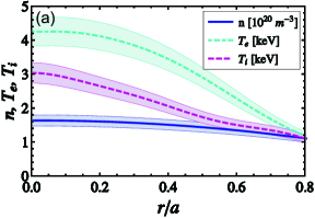
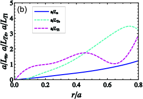
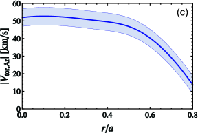
Figure 1: (a) Density and temperature ($n=n_{e}=n_{i}$, $T_{e}$, $T_{i}$) for the electrons and the main ions as functions of $r/a$, with uncertainties represented by the shaded areas. (b) Density- and temperature gradient scale lengths ($a/L_{n}$, $a/L_{Te}$, $a/L_{Ti}$) for the electrons and the main ions as functions of $r/a$. (c) Toroidal rotation of argon as function of $r/a$. Results are taken by averaging over $1.0<t<1.2$ in the studied discharge.

The radial domain we will focus on is $r/a=0.20$–$0.60$, since that is where the ICRH has a considerable impact on the minority temperature anisotropy $\alpha_{T}\equiv T_{\perp}/T_{\|}$ (see Fig. 2(a)). Here, $T_{\perp}$ and $T_{\|}$ are the perpendicular and parallel temperatures of the minority species at the studied flux surface. In this radial domain the electron-ion collision frequency $\nu_{ei}=4\pi n_{e}e^{4}\ln\Lambda/\left[m_{e}^{1/2}(2T_{e})^{3/2}\right]$ (defined according to gyro conventions) varies between $\nu_{ei}=0.02$–$0.05~{}c_{s}/a$, where $\ln\Lambda$ is the Coulomb logarithm, $\epsilon_{0}$ is the vacuum permittivity, and $c_{s}=\left(T_{e}/m_{i}\right)^{1/2}$ is the ion sound speed. Furthermore, the effective normalized electron pressure defined as $\beta_{e}=8\pi n_{e}T_{e}/B^{2}$ varies between $\beta_{e}=0.002$–$0.005$. Although it has been shown that electromagnetic effects can be important for impurity transport even at low $\beta_{e}$ moradiEM , these values are well below the critical value for the onset of kinetic ballooning modes. We will thus restrict ourselves to an electrostatic analysis.

A Poloidally varying equilibrium potential

In Ref. kazakov it was discussed how ICRH affects the poloidal minority ion distribution, and it was shown that when the studied flux surface does not intersect the ICRH resonance, $B\left(\theta\right)\geq B_{c}$, the minority density can be well approximated with a sinusoidal poloidal variation. In Ref. albertICRH it was described how this could give rise to a sinusoidal poloidal variation in the non-fluctuating potential over a flux surface, given by

$$Ze\phi_{E}/T_{z}=-\mathcal{K}\cos\left(\theta-\theta_{0}\right),$$ (1)

where $\mathcal{K}$ is the strength of the asymmetry and $\theta_{0}$ the poloidal location of the minimum of the minority distribution, being $\theta_{0}=\pi$ for ICRH. The effect of the varying potential on turbulent impurity transport has been studied in Refs. albertICRH ; albertTEM ; varenna ; neoVariation , and expressions for the zero-flux impurity density gradient (impurity peaking factor) have been presented.

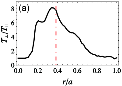
Figure 2: (a) Temperature anisotropy of minority species $\alpha_{T}$ as function of radius computed with transp. The location of the ICRH resonance is marked with a red dashed-dotted line. (b) Non-fluctuating potential as function of poloidal angle at $r/a=0.38$ (red, solid) and $r/a=0.56$ (blue, dashed).

In the present analysis we will not restrict ourselves to the situation when the studied flux surface does not intersect the ICRH resonance, but will also study radial locations where they do intersect. For these flux surfaces a sinusoidal representation is not a good approximation for the varying potential and we will have to resort to a numerical treatment. To model the potential $\phi_{E}$ we start with Eqs. (2) and (3) in Ref. kazakov , describing how the minority density varies over a flux surface

$$n_{H}=\left\{\begin{array}[]{ll}n_{c}\displaystyle\frac{T_{\perp a}}{T_{\perp}},&B>B_{c}\\ n_{c}\displaystyle\left[\frac{T_{\perp a}}{T_{\perp}}+\frac{T_{\perp b}-T_{\perp a}}{T_{\perp}}\left(\frac{T_{\perp}}{T_{\|}}\right)^{1/2}\left(\frac{B_{c}-B}{B_{c}}\right)^{1/2}\right],&B<B_{c}\end{array}\right.,$$ (2)

where

$$\begin{array}[]{l}T_{\perp a}=T_{\perp}\displaystyle\left[\frac{T_{\perp}}{T_{\|}}-\frac{B_{c}}{B}\left(\frac{T_{\perp}}{T_{\|}}-1\right)\right]^{-1}\\ T_{\perp b}=T_{\perp}\displaystyle\left[-\frac{T_{\perp}}{T_{\|}}+\frac{B_{c}}{B}\left(\frac{T_{\perp}}{T_{\|}}+1\right)\right]^{-1}\end{array}$$ (3)

and $n_{c}$ is the minority density on the flux surface at $B=B_{c}$. The poloidal variation in Eqs. (2) and (3) enters through the magnetic field, which under the assumption of large-aspect-ratio ($\epsilon\equiv r/R_{0}\ll 1$) is given by $B=B_{0}/\left(1+r\cos\theta/R_{0}\right)$, where $R_{0}$ is the major radius of the magnetic axis. We define $\tilde{n}_{H}\left(\theta\right)\equiv n_{H}\left(\theta\right)-n_{H0}$ as the deviation from the average minority density over the flux surface. Assuming that the electrons, ions and impurities have a Boltzmann response to the potential, $n_{\alpha}=n_{\alpha 0}\exp(-e_{\alpha}\phi_{E}/T_{\alpha})$ and applying quasi-neutrality it is found that the poloidally varying non-fluctuating potential is given by

$$\frac{Ze\phi_{E}}{T_{z}}=\frac{Z\tilde{n}_{H}/n_{e0}}{{T_{z}}/{T_{e}}+n_{D0}/n_{e0}\left({T_{z}}/{T_{D}}\right)+\sum_{\rm imp}Z_{\rm imp}^{2}\left({n_{\rm imp0}}/{n_{e0}}\right)\left({T_{z}}/{T_{\rm imp}}\right)}$$ (4)

(note that this equation is similar to Eq. (12) in ingessonppcf except that we have not assumed $n_{D0}=n_{e0}$ and $T_{z}=T_{D}$, and that we allow for an arbitrary number of ion species). When all the ion temperatures are equal, Eq. (4) is reduced to $Ze\phi_{E}/T_{z}=Z(\tilde{n}_{H}/n_{e0})/\left({T_{z}}/{T_{e}}-f_{H}+Z_{\mathrm{eff}}\right)$, where $Z_{\mathrm{eff}}=\sum_{i}Z_{i}^{2}n_{i}/n_{e}$ is the effective ion charge. In the case of low-field-side ICRH this potential typically leads to an impurity distribution which is displaced towards the inboard side of the flux surface.

Figure 2 shows the radial profile of the minority species temperature anisotropy, and also illustrates how $Ze\phi_{E}/T_{z}$ from the model in Eq. (4) varies with radius and poloidal angle. Inside the ICRH resonance at $r/a=0.38$, the poloidal variation of $\phi_{E}$ exhibits a sinusoidal-like behavior, but outside it gradually turns into a variation with two peaks. These peaks correspond to the intersections of the flux surface with the almost vertical ICRH resonance layer, where the minority ions are accumulated. The largest magnitude of $\phi_{E}$ almost coincides with the ICRH resonance, and therefore we choose to analyze the radial location $r/a=0.38$ in our further study. However at this location the magnetic shear $s=(r/q)(dq/dr)$, where $q$ is the safety factor, is $s=0.33$ which is a relatively low value. Earlier studies albertICRH ; albertTEM have shown that due to its explicit appearance in the $\mathbf{E}\times\mathbf{B}$-drift term, the magnetic shear can have a strong impact on impurity peaking in the presence of poloidal asymmetries, and in the case of low-field-side ICRH an increased shear is expected to lead to a reduction of the peaking. The magnetic shear increases with radius, and therefore we will also analyze a more outer radial location $r/a=0.56$ where $s=0.78$. We note that from the calculated plasma rotation, we estimate the ratio of the $\mathrm{Mo}^{+32}$ rotation speed to its thermal speed to be around $v_{\mathrm{rot},z}/v_{Tz}\approx 0.8$ at both studied radial locations.

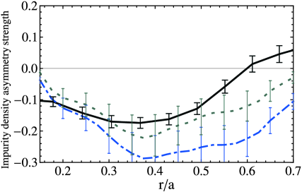
Figure 3: Comparison of the experimentally observed (solid) and numerically computed poloidal asymmetry due to ICRH only (dash-dotted) and with rotation retained (dotted).

The poloidal variation of an impurity species in steady state is approximately given by

$$n_{z}(\theta)\propto\exp\left\{-\frac{Ze\phi_{E}}{T_{z}}-\frac{m_{z}\omega_{z}^{2}(R^{2}-R_{0}^{2})}{2T_{z}}\left[1-\frac{Zm_{i}}{m_{z}}\frac{Z_{\mathrm{eff}}T_{e}}{T_{i}+Z_{\mathrm{eff}}T_{e}}\right]\right\},$$ (5)

where $\omega_{z}$ is the toroidal rotation frequency of the impurities. The long wavelength electrostatic potential $\phi_{E}$ contains only the contribution from the poloidal variation of a non-Boltzmann heated species, and it is given by Eq. (4). The second term in the square bracket in Eq. (5) describes the effect of an electrostatic potential set by the redistribution of all the other ion species on the flux surface due to centrifugal forces. Figure 3 shows the impurity density asymmetry, that is the relative amplitude of the $\cos\theta$ term in an expansion of the poloidal impurity density variation in poloidal harmonics. The experimental value for this quantity is inferred from emissivity measurements on the mid-plane with AXUV, represented by the solid line with error bars, described in Refs. reinke ; reinkeThesis . The dash-dotted line shows the numerically computed asymmetry of the single charge state of $\rm{Mo^{+32}}$, considering only the effect from the minority density variation on the flux surface from ICRH and assuming $Z_{\mathrm{eff}}=1.8$. In most of the plotted region the computed in-out asymmetry is larger than the experimental. This discrepancy is reduced considerably when rotation effects are retained; the dotted curve is calculated keeping the $\omega_{z}^{2}$ part of Eq. (5) assuming that the toroidal rotation speed is similar to that measured for argon. Possible reasons for the remaining disagreement might be uncertainties in the ion composition and in rotation speed, or that the AXUV signal integrates several charge states while the charge state composition varies radially due to the temperature variation. Recent work shows that centrifugal and Coriolis drift effects can have a non-negligible influence on radial impurity transport Casson2010 ; Camenen2009 ; angioni2011 ; angioni2012 , however contributions from these drifts to the impurity peaking factor are estimated to be negligibly small for the case studied here as discussed later in Sec. IV. Therefore we will neglect these effects together with the impact of rotation on the poloidal distribution of particles and concentrate only on the impact of ICRH driven asymmetries.

III Fluxes and mode characteristics

The characteristics of the turbulence present in the studied discharge is analyzed with simulations using the gyrokinetic tool gyro gyro . As discussed in Sec. II we neglect electromagnetic fluctuations, while collisions are included in the simulations and modeled by the Lorentz operator (pitch-angle-scattering). If not otherwise mentioned only the main ion species is included in the simulations, since the presence of impurities in trace content does not affect the turbulence.

From linear gyrokinetic initial-value simulations we obtain the perturbed electrostatic potential $\phi$ and the eigenvalues $\omega=\omega_{r}+i\gamma$ for the most unstable mode, while any sub-dominant modes are neglected. The Miller parametrization of a model Grad-Shafranov magnetic equilibrium is used, where the $\mathcal{O}\left(\epsilon\right)$ corrections to the drift frequencies are retained. We use flux-tube (periodic) boundary conditions, with a 192 point velocity space grid (8 energies, 12 pitch angles and two signs of velocity), the number of radial grid points is 16, and the number of poloidal grid points along particle orbits is 28 for trapped particles. The highest energy grid point is at $m_{i}v^{2}/\left(2T_{i}\right)=6$. Ions are taken to be gyrokinetic while the electrons to be drift kinetic with the mass ratio $\left(m_{i}/m_{e}\right)^{1/2}=60$.

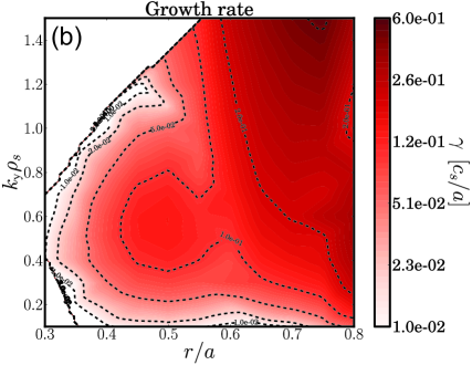
Figure 4: Real mode frequency $\omega_{r}$ (a) and linear growth rate $\gamma$ (b) as functions of $r/a$ and $k_{y}\rho_{s}$ for the linearly most unstable mode, using the initial value solver in gyro.

Figure 4 illustrates a map of linearly unstable modes in $r/a$–$k_{y}\rho_{s}$ space (for $k_{y}\rho_{s}\leq 1.50$ by which the main part of the fluxes is normally driven), where $k_{y}=nq/r$ is the binormal wave number with $n$ being the toroidal mode number, and $\rho_{s0}=c_{s}/\Omega_{i0}$ is the ion sound Larmor radius at $R_{0}$ with $\Omega_{\alpha 0}=e_{\alpha}B_{0}/m_{\alpha}c$ being the cyclotron frequency of species $\alpha$ at $B_{0}$. There are no linearly unstable modes for $r/a\lesssim 0.3$. In the vicinity of the ICRH resonance and up to $r/a\lesssim 0.55$, the plasma is clearly ITG dominated (ITG modes have negative real mode frequency while TEMs have positive real mode frequency according to gyro conventions). For $r/a\gtrsim 0.55$ a TEM branch appears which first is dominant only at higher wave numbers, but for $r/a\gtrsim 0.60$ it dominates the full wave number spectra. However the ITG branch continues to coexist as a sub-dominant branch, and becomes dominant again for low wave numbers closer to the edge. It is worth noting that the linear growth rate of the ITG branch has a local peak close to $r/a=0.50$ and $k_{y}\rho_{s}=0.60$, whereas the growth rate of the TEM branch tends to increase with wave number. This mode is likely to transit to an electron temperature gradient (ETG) mode at even higher wave numbers.

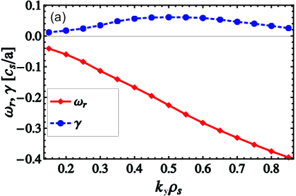
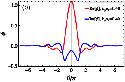
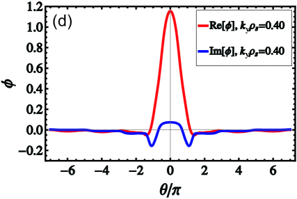
Figure 5: (a, c) Real mode frequency $\omega_{r}$ (red solid line with diamonds) and linear growth rate $\gamma$ (blue dashed line with dots) as functions of $k_{y}\rho_{s}$ at $r/a=0.38$ (a) and $r/a=0.56$ (c). (b, d) Real (red line) and imaginary (blue line) part of the perturbed potential as functions of extended poloidal angle at $r/a=0.38$ (b) and $r/a=0.56$ (d) for $k_{y}\rho_{s}=0.40$.

In Fig. 5 an excerpt of the eigenvalues at $r/a=0.38$ and $r/a=0.56$ is shown, together with the linear eigenfunction for the modes driving the largest fluxes nonlinearly, $k_{y}\rho_{s}\approx 0.40$. Both radial locations are dominated by ITG turbulence at lower wave numbers, and the eigenfunctions exhibit a moderately ballooned structure concentrated to the interval $\theta\in\left[-\pi,\pi\right]$.

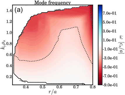
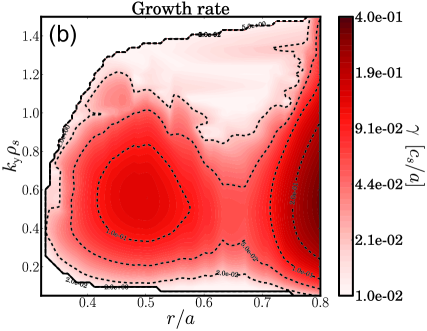
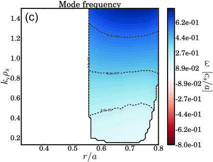
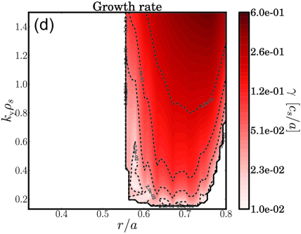
Figure 6: Real mode frequency $\omega_{r}$ (a, c) and linear growth rate $\gamma$ (b, d) as functions of $r/a$ and $k_{y}\rho_{s}$, following the ITG branch (a, b) and the TEM branch (c, d) with the eigenvalue solver in gyro.

To get a wider picture, we trace the two branches observed in Fig. 4 (i.e. the ITG and the TEM branch) using the eigenvalue solver in gyro. The results are illustrated in Fig. 6. We see that the ITG branch exists in the full radial domain where turbulent modes are found (i.e. for $r/a\gtrsim 0.3$) although it is sub-dominant to the TEM branch for $0.55\lesssim r/a\lesssim 0.75$. The branch is limited to $k_{y}\rho_{s}\lesssim 1.40$, and the largest linear growth rates are found for $k_{y}\rho_{s}\approx 0.50$. The TEM branch only exists at $r/a\gtrsim 0.55$. Both its growth rate and linear mode frequency typically increase with increasing wave number.

  

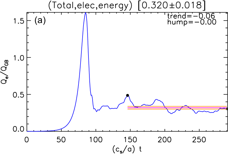
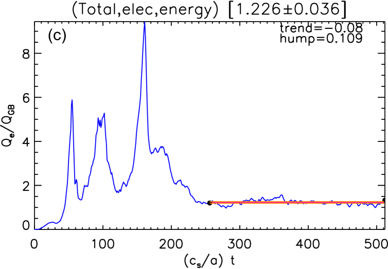
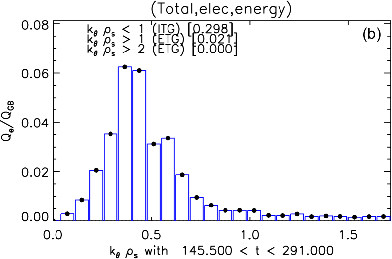
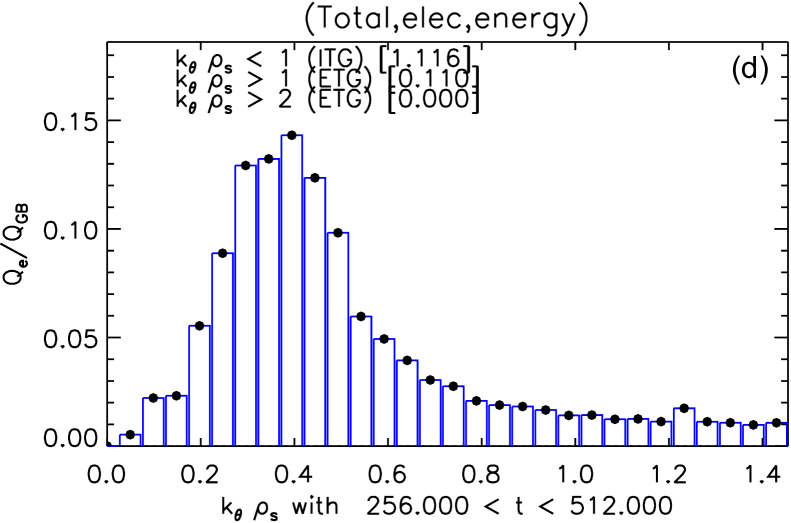
Figure 7: Electron energy fluxes from gyro simulations at $r/a=0.38$ (a, b) and $r/a=0.56$ (c, d). (a, c) Time-evolution of the fluxes. (b, d) Poloidal wave number spectra from the time when the simulations have reached a saturated state.

The nonlinear electrostatic gyro simulations are also performed with gyrokinetic ions and drift kinetic electrons and use the same velocity resolution as the linear simulations. 300 radial grid points are used, and at least 24 toroidal modes to model ${1/5}^{\mathrm{th}}$ of the torus, with the highest resolved poloidal wave number being $k_{y}\rho_{s}\approx 1.5$. The simulations are run with the integration time step $\Delta t=0.01a/c_{s}$ for $t>150a/c_{s}$, when the fluxes have saturated.

Figure 7 shows how the electron energy fluxes evolve over time and the poloidal wave number spectra for both $r/a=0.38$ and $r/a=0.56$. The main part of the fluxes are clearly driven in the regime around $k_{y}\rho_{s}=0.40$, which at both radial locations is ITG dominated (see Fig. 5).

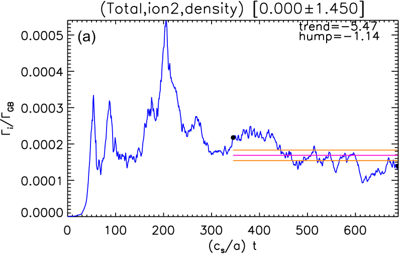
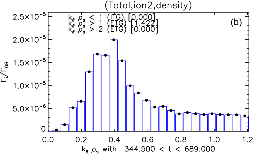
Figure 8: $\mathrm{Mo}^{+32}$ fluxes from gyro simulations at $r/a=0.56$. (a) Time-evolution of the fluxes. (b)  Poloidal wave number spectra from the time when the simulations have reached a saturated state.

To estimate if turbulent impurity fluxes dominate over neoclassical fluxes, we artificially introduce $\mathrm{Mo}^{+32}$ in contents of $n_{z}/n_{e}=2\times 10^{-4}$ at the studied flux surfaces and perform nonlinear gyro simulations. The $\mathrm{Mo}^{+32}$ fluxes from the gyro simulations at $r/a=0.56$ are shown in Fig. 8, note that the largest impurity fluxes are also driven at $k_{y}\rho_{s}=0.40$. We have also performed nonlinear gyro simulations with a different ion composition consisting of $\mathrm{B}^{+5}$, $\mathrm{Ar}^{+18}$ and $\mathrm{Mo}^{+32}$ in contents of $n_{\mathrm{B}}/n_{e}=0.02$, $n_{\mathrm{Ar}}/n_{e}=10^{-3}$ and $n_{\mathrm{Mo}}/n_{e}=2\times 10^{-4}$, at $r/a=0.56$ and for two different values of $a/L_{nz}$. This mix of impurities has similar $Z_{\mathrm{eff}}$ as observed in the experiment, and the combined effects of the dilution result in predicted neutron rate similar to measurements, within uncertainties of the ion temperature. The $\mathrm{Mo}^{+32}$ fluxes from these simulations are of the same size as the fluxes shown in Fig. 8. Thus we make the conclusion that the magnitude of the turbulent $\mathrm{Mo}^{+32}$ fluxes are not sensitive to uncertainties in the ion composition. Neoclassical fluxes have been calculated with neo neo simulations, both including and excluding the temperature anisotropy in the H minority from ICRH as well as plasma rotation, and varying the value of $a/L_{nz}$. Figure 9 shows the neoclassical $\mathrm{Mo}^{+32}$ fluxes as functions of toroidal angular rotation frequency $\omega_{0}$, where the experimentally estimated value is marked by a dotted vertical line. The fluxes are shown for both the case when the temperature anisotropy in H minority is included and the case when it is excluded in the simulation. There is no qualitative difference between the rotation dependence of the neoclassical $\mathrm{Mo}^{+32}$ flux for the two cases. The neoclassical fluxes are sensitive to plasma rotation, but found to be very small for the experimentally estimated value. Comparing the neoclassical fluxes to the turbulent we find that $\Gamma_{\mathrm{Mo}}^{\mathrm{GYRO}}/\Gamma_{\mathrm{Mo}}^{\mathrm{NEO}}\gtrsim 10$ irrespective of the rotation frequency in the neo simulations. Furthermore, we note that both the neoclassical pinch velocity and diffusivity (in all neo simulations performed) are found to be at least an order of magnitude smaller than the corresponding turbulent contributions (from gyro simulations) to the $\mathrm{Mo}^{+32}$ fluxes. tglf tglf simulations show that if the plasma rotation is assumed to be twice the experimental value, turbulent $\mathrm{Mo}^{+32}$ fluxes could be reduced to the same level as the neoclassical.

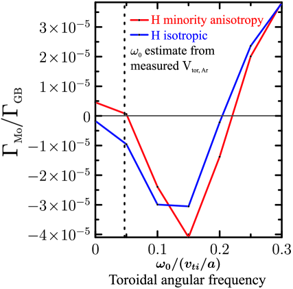
Figure 9: $\mathrm{Mo}^{+32}$ fluxes from neo simulations at $r/a=0.56$, as function of toroidal angular rotation frequency $\omega_{0}$. The experimentally estimated value of $\omega_{0}$ is marked by a dotted vertical line. The blue line shows results from simulations with isotropic H minority species, while the red line shows results from simulations when the temperature anisotropy from ICRH is taken into account.

Tables 1 and 2 show the ion and electron energy fluxes ($Q_{i}$ and $Q_{e}$, respectively) and the electron particle flux $\Gamma_{e}$ normalized to gyro-Bohm units ($Q_{\mathrm{GB}}=n_{e}c_{s}T_{e}\rho_{\ast}^{2}$ and $\Gamma_{\mathrm{GB}}=n_{e}c_{s}\rho_{\ast}^{2}$ where $\rho_{\ast}=\rho_{s}/a$). The turbulent fluxes calculated by nonlinear gyro simulations and the neoclassical values obtained from neo simulations are compared to the result of power balance calculations representing the experimental value. The power balance energy fluxes were obtained by transp simulations and they are estimated to have an uncertainty of $\pm 25\%$. Since there is no core fuelling, the particle sources at these locations are negligibly small, accordingly, the experimental value of $\Gamma_{e}$ is taken to be zero. The neoclassical fluxes are much lower than the simulated turbulent fluxes, as expected for tokamak mid-radius parameters.

The turbulent ion energy fluxes at the nominal value of $a/L_{Ti}$ are significantly higher than the experimental fluxes. However, the transport is very stiff, i.e. it is sensitive to small changes in local plasma parameters, especially $a/L_{Ti}$, as it is often observed in ITG dominated plasmas. Tables 1 and 2 also show the fluxes at $a/L_{Ti}\pm 10\%$. Without performing a full sensitivity study to different plasma parameters, as that is outside the scope of the present paper, from the observed stiffness of the transport, it is reasonable to believe that the ion energy fluxes can be matched by reducing $a/L_{Ti}$ and adjusting other parameters, including impurity composition, within their experimental uncertainty (noting that $a/L_{Ti}$ has an uncertainty of roughly $20\%$). The gyro electron energy fluxes are comparable to the experimental values already at nominal $a/L_{Ti}$, however it seems unlikely that both $Q_{i}$ and $Q_{e}$ could be matched to experiment simultaneously without performing a multi-scale gyrokinetic analysis. A stronger electron than ion heat transport channel has previously been observed in ICRH heated C-Mod experiments porkolab ; howard . Also, main ion dilution can significantly reduce the ion energy fluxes, as found in Ref. porkolab . In the nonlinear gyro simulations at $r/a=0.56$ described earlier, including the lower-$Z$ (more diluting) impurities $\mathrm{B}^{+5}$ and $\mathrm{Ar}^{+18}$, we find that the energy fluxes are significantly reduced. The values are given in Tab. 2. $Q_{i}$ becomes substantially closer to its experimental value, whereas $Q_{e}$ is reduced to lower than the experimental value. To study the impurity transport using our linear model, it is not necessary to use the exact parameters that would match the experimental fluxes, since the impurity peaking factor calculated in our linear model presented in the next section is only weakly sensitive to the mode characteristics.

Case	$Q_{i}~{}\left[Q_{\mathrm{GB}}\right]$	$Q_{e}~{}\left[Q_{\mathrm{GB}}\right]$	$\Gamma_{e}~{}\left[\Gamma_{\mathrm{GB}}\right]$
gyro $a/L_{Ti}$ -10%	$0.895\pm 0.098$	$0.18\pm 0.02$	$0.012\pm 0.001$
GYRO	$\mathbf{1.58}\pm 0.092$	$\mathbf{0.32}\pm 0.018$	$\mathbf{0.017}\pm 0.002$
gyro $a/L_{Ti}$ +10%	$2.03\pm 0.18$	$0.40\pm 0.034$	$0.024\pm 0.003$
neo	$9.2\times 10^{-3}$	$4.2\times 10^{-4}$	$9.3\times 10^{-5}$
Power balance	$0.084$	$0.28$	$0$

Table 1: Comparison of simulated particle- and energy fluxes from gyro (turbulent) and neo (neoclassical), and experimentally measured fluxes, at $r/a=0.38$. Also given are gyro fluxes when $a/L_{Ti}$ has been artificially increased or decreased by 10%. Fluxes are given in Gyro-Bohm units and $\rho_{\ast}=5.4\times 10^{-3}$. Note that positive (negative) flux is outward (inward).

Case	$Q_{i}~{}\left[Q_{\mathrm{GB}}\right]$	$Q_{e}~{}\left[Q_{\mathrm{GB}}\right]$	$\Gamma_{e}~{}\left[\Gamma_{\mathrm{GB}}\right]$
gyro $a/L_{Ti}$ -10%	$1.20\pm 0.032$	$0.81\pm 0.016$	$-0.22\pm 0.004$
GYRO	$\mathbf{1.96}\pm 0.07$	$\mathbf{1.23}\pm 0.04$	$\mathbf{-0.29}\pm 0.007$
gyro $a/L_{Ti}$ +10%	$3.56\pm 0.12$	$2.18\pm 0.088$	$-0.38\pm 0.014$
gyro $\mathrm{B}$/$\mathrm{Ar}$/$\mathrm{Mo}$	$0.64\pm 0.046$	$0.38\pm 0.031$	$-0.13\pm 0.008$
neo	$0.013$	$1.1\times 10^{-3}$	$1.8\times 10^{-4}$
Power balance	$0.38$	$0.88$	$0$

Table 2: Comparison of simulated particle- and energy fluxes from gyro (turbulent) and neo (neoclassical), and experimentally measured fluxes, at $r/a=0.56$. Also given are gyro fluxes when $a/L_{Ti}$ has been artificially increased or decreased by 10%, and when the ion composition has been modified to include $\mathrm{B}^{+5}$, $\mathrm{Ar}^{+18}$ and $\mathrm{Mo}^{+32}$ in contents of $n_{\mathrm{B}}/n_{e}=0.02$, $n_{\mathrm{Ar}}/n_{e}=10^{-3}$ and $n_{\mathrm{Mo}}/n_{e}=2\times 10^{-4}$. Fluxes are given in Gyro-Bohm units and $\rho_{\ast}=4.4\times 10^{-3}$. Note that positive (negative) flux is outward (inward).

IV Impurity density peaking

A semi-analytical linear gyrokinetic model for the zero flux density gradient of impurities present in trace quantities was introduced in Ref. fulop and later extended to include parallel streaming effects in the high-$Z$ limit in Ref. varenna , where the effect of a poloidally varying, non-fluctuating electrostatic potential $\phi_{E}$ is included with $e_{z}\phi_{E}/T_{z}\sim\mathcal{O}\left(1\right)$. From Fig. 2 we note that this ordering is valid for the studied ICRH discharge. In Ref. albertTEM the model was applied to TEMs, and demonstrated the ability to reproduce trends of nonlinear gyro simulations in the poloidally symmetric case. An important result was that the strength of the asymmetry $\mathcal{K}$ and the magnetic shear $s$ are key parameters in determining the size of the effect, since they both appear as explicit factors in the $\mathbf{E}\times\mathbf{B}$ drift which arises due to the poloidal variation in the potential. References varenna ; albertTEM assumed a sinusoidal variation in the non-fluctuating potential of the form in Eq. (1), but as discussed in Sec. II we need to allow for a more general form in the present analysis. Furthermore, similarly to Ref. varenna we assume a low-beta plasma and large-aspect-ratio, but in the present treatment we will allow for shaping effects in form of plasma elongation, $\kappa$. In Ref. skyman2014 the impact of shaping effects on the impurity peaking factor is investigated, and it is found that considering a realistic geometry can significantly modify the high-$Z$ peaking factor as compared to using a simplified circular geometry. Furthermore it is argued that the main effect can be attributed to elongation. We note that employing Miller type parametrization an elliptical flux surface with elongation $\kappa$ is given above Eq. (A1), where $\theta$ is not the geometrical poloidal angle $\Theta$, but an angle-like parameter which also varies as $\theta:0\rightarrow 2\pi$, and is related to $\Theta$ by $\tan\Theta=\kappa\tan\theta$.

The linearized gyrokinetic equation for the non-adiabatic perturbed impurity distribution $g_{z}$ is given by

$$\left.\frac{v_{\parallel}}{qR}\frac{\partial{g}_{z}}{\partial\theta}\right|_{\mathcal{E},\mu}-i(\omega-\omega_{Dz}-\omega_{E}){g}_{z}-C[g_{z}]=-i\frac{Zef_{z0}}{T_{z}}\left(\omega-\omega_{\ast z}^{T}\right)\phi J_{0}(z_{z}).$$ (6)

Here $f_{z0}=n_{z0}(m_{z}/2\pi T_{z})^{3/2}\exp(-\mathcal{E}/T_{z})$ is the equilibrium Maxwellian distribution function, $\mathcal{E}=m_{z}v^{2}/2+Ze\phi_{E}$ is the total unperturbed energy, $\mu=m_{z}v_{\perp}^{2}/\left(2B\right)$ is the magnetic moment, $n_{z}(\mathbf{r})=n_{z0}\exp[-Ze\phi_{E}(\mathbf{r})/T_{z}]$ is the poloidally varying impurity density where $n_{z0}$ is a flux function, and $\phi$ is the perturbed potential. $J_{0}$ is the Bessel function of the first kind, $z_{z}=k_{\perp}v_{\perp}/\Omega_{z}$, and $k_{\perp}=\left(1+s^{2}\theta^{2}\right)^{1/2}k_{y}$. $\omega_{Dz}=-2k_{y}T_{z}(x_{\perp}^{2}/2+x_{\parallel}^{2})\mathcal{D}\left(\theta\right)/\left(m_{z}\Omega_{z}R\kappa\right)$ is the magnetic drift frequency, where $\mathcal{D}\left(\theta\right)=\cos{\theta}+s\theta\sin{\theta}$ and $x=v/v_{Tz}$ represents velocity normalized to the thermal speed $v_{Tz}=(2T_{z}/m_{z})^{1/2}$, whereas $\omega_{\ast z}=-k_{y}T_{z}/ZeB\kappa L_{nz}$ is the diamagnetic frequency and $\omega_{\ast z}^{T}=\omega_{\ast z}\left[1+\left(x^{2}-3/2\right)L_{nz}/L_{Tz}\right]$. $\omega_{E}$ is the $\mathbf{E}\times\mathbf{B}$ drift frequency of the particles in the non-fluctuating electrostatic field given by

$$\omega_{E}=-\frac{k_{y}}{B}\frac{s\theta}{r\kappa}\frac{\partial\phi_{E}}{\partial\theta},$$ (7)

if radial variation of $\phi_{E}$ is neglected, the term was derived in Appendix A of Ref. albertICRH . $C[\cdot]$ is the collision operator.

The impurity peaking factor is found by solving Eq. (6) and requiring that the linear impurity flux $\Gamma_{z}$ should vanish

$$0=\left\langle\Gamma_{z}\right\rangle\equiv\left\langle\mathrm{Im}\left[-\frac{k_{y}}{B}\hat{n}_{z}\phi^{\ast}\right]\right\rangle=\left\langle\mathrm{Im}\left[-\frac{k_{y}}{B}\int d^{3}vJ_{0}\left(z_{z}\right)g_{z}\phi^{\ast}\right]\right\rangle.$$ (8)

A perturbative solution to Eq. (6) in the small parameter $Z^{-1/2}\ll 1$ was presented in Ref. varenna , keeping terms up to $\mathcal{O}(Z^{-1})$ in the expansion of ${g}_{z}$. The solution orders $\omega_{Dz}/\omega$, $\omega_{\ast z}^{T}/\omega$, $\omega_{E}/\omega$ and $J_{0}(z_{z})-1\approx-z_{z}^{2}/4$ as $\sim\!1/Z$ small (assuming $m_{z}/m_{i}\sim Z$), and models collisions by the full linearized impurity-impurity collision operator $C_{zz}^{(l)}$. Furthermore it is also assumed that $\phi$ and $\omega$ are known from the solution of the linear gyrokinetic-Maxwell system (obtained from gyro) and that they are unaffected by the presence of trace impurities, and the non-fluctuating potential. We refer to Ref. varenna for more details. A semi-analytical expression for the impurity peaking factor is given in Eq. (8) of Ref. varenna . In the present analysis we will adopt the same perturbative solution, but keep the final solution for the peaking factor numerical to account for a more complicated non-fluctuating potential and $\mathcal{O}\left(\epsilon\right)$ corrections. Since it is shown in Ref. varenna that collisions do not affect impurity peaking to order $1/Z$, we will neglect them here for simplicity. Writing $g_{z}=g_{0}+g_{1}+g_{2}+\mathcal{O}\left(1/Z^{3/2}\right)$, the 0^th order solution is given by $g_{0}=Ze\phi f_{z0}/T_{z}$, the 1^st order solution by $g_{1}=-iZef_{z0}v_{\|}\left(\partial\phi/\partial\theta\right)/\left(T_{z}\omega qR\right)$, and the 2^nd order solution by $g_{2}=\left(\omega_{Dz}+\omega_{E}\right)g_{0}/\omega+v_{\|}\left(\partial g_{1}/\partial\theta\right)/\left(i\omega qR\right)-Ze\phi f_{z0}\left(\omega z_{z}^{2}/4+\omega_{\ast z}^{T}\right)/\left(\omega T_{z}\right)$. Since $g_{0}$ is an adiabatic response and $g_{1}$ disappears when integrating over velocity space, only $g_{2}$ contributes to the impurity fluxes. Furthermore, since the impurity density varies over the flux surface, what we calculate is an effective impurity peaking factor $a/L_{nz}^{0}=a/L_{nz}^{\ast}$ when $\left\langle\Gamma_{z}\right\rangle=0$, where $a/L_{nz}^{\ast}=\langle a/L_{nz}\rangle_{\phi}$ is a weighted flux surface average with $\langle\dots\rangle_{\phi}=\langle\dots\mathcal{N}|\phi|^{2}\rangle/\langle\mathcal{N}|\phi|^{2}\rangle$ and $\mathcal{N}(\theta)=\exp{[-e_{z}\phi_{E}/T_{z}]}$.

Regarding the effects of a constant elongation, we note that $\kappa>1$ reduces the magnetic, the non-fluctuating $\mathbf{E}\times\mathbf{B}$ and the diamagnetic drift terms by a factor $1/\kappa$, while it does not affect the parallel streaming term, as shown in Appendix A. In terms of the impurity peaking factor, the elongation increases the parallel streaming term by a factor $\kappa$, but it leaves the drift contributions unchanged. Thus, in ITG dominated plasmas where parallel streaming acts as to increase the peaking factor, the peaking factor is expected to be higher than in a similar circular cross section plasma, especially in the core where $q^{2}$ is not too large.

We consider a single representative linear mode, which is the mode at $k_{y}\rho_{s}=0.40$ driving the largest fluxes nonlinearly (see Fig. 8). Note that since we are using a linear model, only the most unstable mode is considered and any sub-dominant modes are neglected. At $r/a=0.56$ there exists a sub-dominant TEM with very low growth rate (see Fig. 6). From a potential frequency response analysis of the nonlinear simulations we found that fluctuations with frequencies in the electron diamagnetic direction have negligibly small amplitudes, thus we do not expect that neglecting the transport driven by the sub-dominant TEM affects the results significantly.

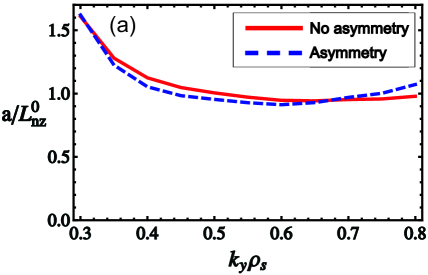
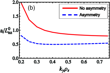
Figure 10: $\mathrm{Mo}^{+32}$ peaking factor at $r/a=0.38$ (a) and at $r/a=0.56$ (b) as functions of $k_{y}\rho_{s}$. Red solid line is the peaking factor when the poloidally varying non-fluctuating potential is excluded from the model, while blue dashed line is the peaking factor when the potential is included.

Figure 10 shows the model $\mathrm{Mo}^{+32}$ peaking factor at $r/a=0.38$ and $r/a=0.56$ as function of binormal wave number, when the poloidally varying non-fluctuating potential is excluded and included in the model. For $k_{y}\rho_{s}=0.40$, the mode driving the largest fluxes, the peaking factor is practically unaffected by the inclusion of the potential at $r/a=0.38$, while at $r/a=0.56$ it decreases from ${\color[rgb]{0,0,0}a/L_{nz}^{0}}=0.93$ to ${\color[rgb]{0,0,0}a/L_{nz}^{0}}=0.49$. One of the reasons for the weak effect at $r/a=0.38$ is a moderate value of the magnetic shear $s=0.33$, which makes the $\mathbf{E}_{\theta}\times\mathbf{B}_{\varphi}$-drift term relatively small. At $r/a=0.56$ the magnetic shear is $s=0.78$ and the $\mathbf{E}_{\theta}\times\mathbf{B}_{\varphi}$-drift is stronger. However, the approximate proportionality of the $\mathbf{E}_{\theta}\times\mathbf{B}_{\varphi}$-drift to magnetic shear in itself cannot explain the large relative increase in the impact of poloidal asymmetries. Figure 10 is calculated retaining $\mathcal{O}(\epsilon)$ corrections to the peaking factor. We note, that the reduction of the peaking factor due to poloidal asymmetry effects is found to be much smaller when a simplified model neglecting $\mathcal{O}(\epsilon)$ corrections is used for the calculation. This suggests that these corrections may be important for some set of parameters, as it is the case here.

Figure 11 shows the comparison of the peaking factors as calculated above to the experimental range. The codes GENTRAN gentran and STRAHL strahl were used to constrain the impurity profile from the measured emission data mattAPS . GENTRAN solves for the steady state charge state density profiles given assumed input impurity diffusion and convection profiles. We assume a flat diffusion profile, and the convection profile is found using a least-squares minimization routine that best matches the time-averaged neon-like molybdenum emissivity profile for $0.10<r/a<0.53$. Assuming a finite range for diffusivities, 0.5 to 1.8 $\mathrm{m}^{2}/\mathrm{s}$, and considering the uncertainties in the contribution due to charge exchange recombination provides a range for the experimental peaking factors can be calculated that are consistent with experiment. Figure 11 shows two uncertainty ranges for the impurity peaking factor. The light gray area is based purely on GENTRAN simulations and use less restrictive assumptions, allowing larger uncertainties. At the same time, the diffusion and convection profiles calculated by GENTRAN can be used as inputs for STRAHL simulations. STRAHL computes the time-evolving charge state density profiles, in particular, it can predict the exponential decay times of the impurity density during the laser blow off experiment. The dark-gray region in Fig. 11 reflects the molybdenum density profiles for which the decay times predicted by STRAHL are within the experimental uncertainty. We note that, although it would be ideal to use STRAHL alone to simulate the full time history and constrain the diffusion and convection profiles, uncertainties in the atomic physics data for molybdenum currently prevent using this proven work flow. The theoretically predicted linear peaking factors (corresponding to $k_{y}\rho_{s}=0.40$) at the two studied radial locations are shown with arrows. The arrows from the left (blue) include the poloidal asymmetry effects, while the arrows from the right are calculated assuming no ICRH driven poloidal asymmetries (these correspond to the blue and red curves of Fig. 10, respectively).

At $r/a=0.38$, the calculated peaking factors – which, in this case, are almost the same with and without asymmetries – fall within the more restrictive experimental range. However, the ones calculated for $r/a=0.56$ strongly underestimate the experimental impurity peaking factor, even when the less restrictive range is considered. Note that, although we neglected rotation effects in the calculation, this level of discrepancy likely cannot be explained by rotation effects. Using the model presented in Ref. angioni2012 , drift contributions due to rotation on the impurity peaking are estimated to be an order of magnitude smaller then the peaking factors calculated here. As seen in Fig. 3, at this radial location the poloidal variation of the impurity density is still not dominated by rotation effects, although these become comparable to the ICRH-induced effects. Accordingly the “no asymmetry” result (red arrow from right in Fig. 11) may be considered as an estimate for the peaking factor in this case. As long as we assume that the linear peaking factor is a good approximation to the nonlinear one, the strong discrepancy observed makes it clear that in the outer radial location the impurity peaking is determined by some physical mechanism not included in our model. To obtain such a large peaking factor as seen for $r/a=0.56$, there should be a drift frequency in the gyrokinetic equation affecting the impurity dynamics that is several times larger than the diamagnetic drift frequency.

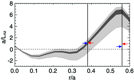
Figure 11: Radial variation of the impurity peaking factor. Light and dark gray shaded areas represent the experimental values calculated using a less and a more restricting set of assumptions on the uncertainties. Vertical bars mark the two studied radii. Arrows represent the theoretical estimates for the peaking factor at these radial locations; from the left (blue arrows): with asymmetries, from the right (red arrows): without asymmetries.

The discrepancy between the experiment and the simulation at the outer radius might be due to the increasing importance of atomic physics processes. In Ref. mattAPS the neutral fraction (which is not a measured quantity) is shown to have a significant impact on the radial distribution of molybdenum with $Z>30$, especially outside $r/a=0.5$. On the other hand, the gyrokinetic modeling of the impurity transport considers only a single charge state of the impurity and neglects volumetric sources due to ionization and recombination. Consequently it is, although important to point out, not completely unexpected that we do not find agreement between experiment and modeling at the outer core. This does illustrate the role of uncertainties in atomic physics data in complicating efforts at validating gyrokinetic models of high-$Z$ impurity transport.

Sensitivity analysis of impurity peaking

In this subsection we investigate the sensitivity of the impurity peaking factor to the plasma effective charge, by introducing $\mathrm{B}^{+5}$, $\mathrm{Ar}^{+18}$ and $\mathrm{Mo}^{+32}$ in contents of $n_{\mathrm{B}}/n_{e}=0.02$, $n_{\mathrm{Ar}}/n_{e}=10^{-3}$ and $n_{\mathrm{Mo}}/n_{e}=2\times 10^{-4}$, resulting in a plasma effective charge of $Z_{\mathrm{eff}}=1.90$. Including the above mentioned impurities, Eq. (4) for the non-fluctuating potential becomes

$$\frac{Ze\phi_{E}}{T_{z}}=\frac{Z\tilde{n}_{H}/n_{e0}}{{T_{z}}/{T_{e}}+({T_{z}}/{T_{i}})({n_{i0}}/{n_{e0}})+{n_{z0}Z^{2}}/{n_{e0}}+{n_{\mathrm{B}0}Z_{\mathrm{B}}^{2}T_{z}}/\left(n_{e0}T_{\mathrm{B}}\right)+{n_{\mathrm{Ar}0}Z_{\mathrm{Ar}}^{2}T_{z}}/\left(n_{e0}T_{\mathrm{Ar}}\right)}.$$ (9)

The inclusion of the $\mathrm{B}^{+5}$ and $\mathrm{Ar}^{+18}$ impurities lead to a reduction of the non-fluctuating potential, and accordingly also the peaking factor is slightly increased in the poloidally asymmetric case, as shown in Fig. 12(c) for the radial location $r/a=0.56$. Interestingly, the TEM which was dominant for higher wave number in Fig. 5 at $r/a=0.56$ disappears if the above mentioned impurities are included, as illustrated in Fig. 12(a).

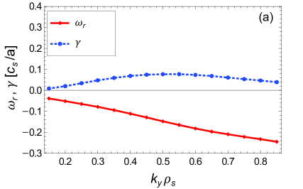
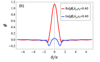
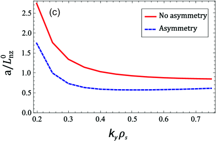
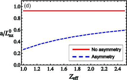
Figure 12: (a) Real mode frequency $\omega_{r}$ (red solid line with diamonds) and linear growth rate $\gamma$ (blue dashed line with dots) as functions of $k_{y}\rho_{s}$ at $r/a=0.56$, for a plasma with $\mathrm{B}^{+5}$, $\mathrm{Ar}^{+18}$ and $\mathrm{Mo}^{+32}$ introduced in trace quantities and $Z_{\mathrm{eff}}=1.90$. (b) Real (red line) and imaginary (blue line) part of the perturbed potential as functions of extended poloidal angle at $r/a=0.56$ and $k_{y}\rho_{s}=0.40$ for the corresponding plasma. (c) $\mathrm{Mo}^{+32}$ peaking factor at $r/a=0.56$ as function of $k_{y}\rho_{s}$ for the corresponding plasma. Red solid line is the peaking factor when the poloidally varying non-fluctuating potential is excluded from the model, while blue dashed line is the peaking factor when the potential is included. (d) $\mathrm{Mo}^{+32}$ peaking factor at $r/a=0.56$ and $k_{y}\rho_{s}=0.40$ as function of $Z_{\mathrm{eff}}$.

Figure 12(d) shows how the $\mathrm{Mo}^{+32}$ peaking factor varies with $Z_{\mathrm{eff}}$, under the assumption that the turbulence is unaffected by the change in impurity content which is expected as long as all impurity species are in trace quantities. The figure illustrates that the peaking factor is sensitive to the effective plasma charge, which is also evident from Eq. (4). To be able to predict the magnitude of the poloidal asymmetry in the non-fluctuating potential a good estimate of $Z_{\mathrm{eff}}$ is required. However, neither the inclusion of lower $Z$ impurities or changing the effective charge produces strong enough deviation in the peaking factor to explain the experimentally observed very high value.

V Discussion and conclusions

We have performed a gyrokinetic study of the turbulent transport of highly charged molybdenum impurity in an off-axis ICRH heated discharge on Alcator C-Mod. The discharge is part of an experiment series to study the effect of ICRH induced asymmetries on high-$Z$ impurity transport, where multiple radiation imaging diagnostics follow the spatio-temporal dynamics of molybdenum introduced using laser blow-off.

We find that for inner core radii ($r/a<0.5$) there is a significant ICRH-induced in-out asymmetry, while further out this asymmetry is not as pronounced or driven by centrifugal effects. This trend is partly due to the ICRH resonance location determining the poloidally varying non-fluctuating potential and partly due to rotation effects, even though this discharge has a low rotation speed on the diamagnetic level. We perform eigenvalue solver gyrokinetic simulations with gyro, resolved radially and in $k_{y}\rho_{s}$, which show unstable microinstabilities for $r/a>0.3$. In the inner core ($r/a<0.55$) the turbulence is ITG dominated, while in the outer core an ITG and a higher wave number TEM coexist.

Nonlinear gyrokinetic simulations at the nominal values of plasma parameters significantly overestimate the ion heat transport at the studied radial locations, however the transport is found to be rather stiff. The ion heat transport in the simulations is brought significantly closer to the experimental value by modifying the ion composition to include lower-$Z$, more diluting, impurities. The electron energy transport can be matched when the ion temperature gradient is changed within a $10\%$.

At the inner radius studied, $r/a=0.38$, the impurity peaking factor calculated using a linear gyrokinetic model matches the experiment within uncertainties. However the effect of ICRH-induced asymmetries is negligibly small due to the relatively low magnetic shear. The difference between the calculated peaking factors with and without poloidal asymmetries are too close to be experimentally distinguishable. At the outer radius, $r/a=0.56$, the magnetic shear is higher and the effect of ICRH is still strong enough to induce a stronger reduction in the impurity peaking factor. However, independently on whether poloidal asymmetries are considered or not, and considering a reasonable sensitivity to ion composition and gradients, the range of calculated impurity peaking factors (${\color[rgb]{0,0,0}a/L_{nz}^{0}}\approx 0.2-1.7$) strongly underestimates the experimentally observed very high impurity peaking factor (${\color[rgb]{0,0,0}a/L_{nz}^{0}}\approx 6$). This suggests that there is some mechanism in the outer core strongly affecting impurity transport, not presently included in our model. Pure neoclassical transport could generate such a large peaking. However, comparing nonlinear gyrokinetic simulations and neoclassical simulations we show that neoclassical transport is too small to be a good candidate. The effects of the weak rotation in the experiment, which we estimated, are not expected to qualitatively change the picture either. On the other hand, previous studies showing a sensitivity of the radial profiles of high ionization states of molybdenum to neutral fraction indicate that atomic physics processes may be inducing a systematic error in interpreting experimental results at mid-radius.

Although the presented study of an Alcator C-Mod experiment seems to point towards a conclusion that the ICRH-driven poloidal asymmetry may not be a tool to control impurity transport, we note that the peaking factors we find strongly depend on magnetic shear, and are affected by the radial region where atomic physics becomes important. In larger devices with hotter plasmas, such as JET or ITER, there might be bigger room to harvest the favorable effects of ICRH-driven asymmetries on turbulent transport. In fact, ICRH is routinely applied on JET to avoid an uncontrolled impurity accumulation event in the core, and it is still not clear what physics effect plays the dominant role in that case. Furthermore, in the deep core, where turbulent transport seems to be absent, the effect of these asymmetries on neoclassical transport – which is an area yet to be explored in detail – may also be beneficial.

Appendix A: Drift frequencies in a large aspect ratio, elongated equilibrium

In this section we evaluate the effect of a constant elongation $\kappa$ on the different terms in the gyrokinetic equation assuming large aspect ratio $\epsilon=r/R_{0}\ll 1$ and unshifted flux surfaces ($R_{0}$ is independent of $r$).

Defining a coordinate basis $\{r,\theta,\zeta\}$ through $x=R\cos(-\zeta)$, $y=R\sin(-\zeta)$, $z=\kappa r\sin\theta$, with $R=R_{0}+r\cos\theta$, where $\{x,y,z\}=\mathbf{r}$ is the Cartesian system, we find that the Jacobian is

$$\mathcal{J}=\left|\frac{\partial(x,y,z)}{\partial(r,\theta,\zeta)}\right|=r\kappa(R_{0}+r\cos\theta)=rR\kappa.$$ (A1)

We may also calculate the Jacobian of the coordinate basis $\{\psi,\theta,\zeta\}$ where $r=r(\psi)$ with the poloidal magnetic flux $2\pi\psi$, to find

$$\mathcal{J}_{\psi}=\left(\partial\psi/\partial r\right)^{-1}\mathcal{J}\quad=\left(B\mathbf{b}\cdot\nabla\theta\right)^{-1},$$ (A2)

where the magnetic field $\mathbf{B}=B\mathbf{b}$ with $B=|\mathbf{B}|$. The gradient vectors can be evaluated to be

$$\nabla r= \left(\frac{\partial\mathbf{r}}{\partial\theta}\times\frac{\partial\mathbf{r}}{\partial\zeta}\right)\mathcal{J}^{-1}=\left\{\cos\theta\cos\zeta,\,-\cos\theta\sin\zeta,\,\kappa^{-1}\sin\theta\right\},$$

$$\nabla\theta= \left(\frac{\partial\mathbf{r}}{\partial\zeta}\times\frac{\partial\mathbf{r}}{\partial r}\right)\mathcal{J}^{-1}=\frac{1}{r}\left\{-\sin\theta\cos\zeta,\,\sin\theta\sin\zeta,\,\kappa^{-1}\cos\theta\right\},$$ (A3)

$$\nabla\zeta= \left(\frac{\partial\mathbf{r}}{\partial r}\times\frac{\partial\mathbf{r}}{\partial\theta}\right)\mathcal{J}^{-1}=\frac{1}{R_{0}+r\cos\theta}\left\{-\sin\zeta,\,-\cos\zeta,\,0\right\},$$

from which we find

$$\eqalign{|\nabla r|^{2}=&1-(1-1/\kappa^{2})\sin^{2}\theta,\\ |\nabla\theta|^{2}=&\left[1+(\kappa^{2}-1)\sin^{2}\theta\right]/(r\kappa)^{2},\\ |\nabla\zeta|^{2}=&1/R^{2},\\ \nabla r\cdot\nabla\theta=&\left[(1-\kappa^{2})\cos\theta\sin\theta\right]/(r\kappa^{2}),}$$ (A4)

and $\nabla r\cdot\nabla\zeta=0=\nabla\theta\cdot\nabla\zeta$. The strength of the poloidal magnetic field is given by $B_{p}=|\nabla\psi|/R=(\partial\psi/\partial r)|\nabla r|/R=B_{p0}\left[1-(1/\kappa^{2})\sin^{2}\theta\right]^{1/2}$, with $B_{p0}=R_{0}^{-1}\partial\psi/\partial r$.

We introduce the binormal variable $\alpha$ through the following representation of the magnetic field $\mathbf{B}=\nabla\alpha\times\nabla\psi$. This representation is consistent with the usual $\mathbf{B}=\nabla\zeta\times\nabla\psi+I\nabla\zeta$ when $\alpha=\zeta-\int_{0}^{\theta}d\theta I/(R^{2}\mathbf{B}\cdot\nabla\theta)\approx\zeta-q\theta$, where we define the safety factor as $q=B_{0}r\kappa/(R_{0}B_{p0})$ and neglect $\epsilon$ corrections.

When the fluctuating quantities X have the form $X=X(\theta)\exp\{-i\omega t+ik_{\psi}\psi-in\alpha\}$, where $\theta$ is the ballooning angle, the perpendicular wave number defined by $\nabla_{\perp}X=i\mathbf{k}_{\perp}X$ can be written as

$$\mathbf{k}_{\perp}=[k_{\psi}+n\theta(\partial q/\partial\psi)]\nabla\psi-n(\nabla\zeta-q\nabla\theta)=k_{y}[r\nabla\theta+s(\theta-\theta_{0})\nabla r],$$ (A5)

where we introduced the binormal wave number $k_{y}=nq/r$, $\theta_{0}=-k_{\psi}R_{0}B_{p0}/k_{y}s$, and recalled the definitions $s=(r/q)\partial q/\partial r$ and $R_{0}B_{p0}=\partial\psi/\partial r$, furthermore, in $\mathbf{k}_{\perp}$ we neglected a term of the size $k_{y}r/(qR_{0})$ as small in $\epsilon$.

From Eq. (A5) we find the perpendicular wave number appearing in finite Larmor radius terms is given by $k_{\perp}=k_{y}\left[r^{2}|\nabla\theta|^{2}+s^{2}(\theta-\theta_{0})^{2}|\nabla r|^{2}+2rs(\theta-\theta_{0})\nabla r\cdot\nabla\theta\right]^{1/2}$, where the gradient expressions are given by Eq. (A4).

Then we turn to the drift terms appearing in Eq. (6) assuming that $\mathbf{k}_{\perp}$ is orthogonal to $\nabla r$ at the outboard mid-plane, that is, $\theta_{0}=0$. First we consider the radial $\mathbf{\mathbf{E}\times\mathbf{B}}$ drifts

$$\omega_{E}=\left[\frac{1}{B^{2}}\mathbf{B}\times\nabla\theta\frac{\partial\phi_{E}}{\partial\theta}\right]\cdot\mathbf{k}_{\perp}=\frac{k_{y}}{B^{2}}\frac{\partial\phi_{E}}{\partial\theta}\frac{\partial\psi}{\partial r}\left[(\nabla\alpha\times\nabla r)\times\nabla\theta\right]\cdot\left[s\theta\nabla r+r\nabla\theta\right],$$ (A6)

where we write $\mathbf{B}=(\partial\psi/\partial r)\nabla\alpha\times\nabla r$, and used that $\partial\phi_{E}/\partial r$ does not contribute to the radial drift and $(\partial/\partial\alpha|_{\theta,r})\phi_{E}=\partial\phi_{E}/\partial\zeta=0$. Using the definition of $\alpha$ we find

$$\omega_{E}=C\left\{\left[\left(\nabla\zeta-q\nabla\theta-\theta(\partial q/\partial r)\nabla r\right)\times\nabla r\right]\times\nabla\theta\right\}\cdot(s\theta\nabla r+r\nabla\theta),$$ (A7)

with $C=(k_{y}/B^{2})(\partial\phi_{E}/\partial\theta)(\partial\psi/\partial r)$. After some algebra Eq. (A7) reduces to

$$\omega_{E}=-Cqs\theta\left[|\nabla r|^{2}|\nabla\theta|^{2}-(\nabla r\cdot\nabla\theta)^{2}\right].$$ (A8)

Using Eq. (A4), the expression in the square bracket in Eq. (A8) can be simplified to $1/(r\kappa)^{2}$, which, together with $\partial\psi/\partial r\approx Br\kappa/q$ yields the result, Eq. (7).

Next we evaluate the magnetic drift frequency of species $a$ in the $\beta\ll 1$ limit, when the magnetic drift velocity is given by

$$\mathbf{v}_{Ma}=\frac{\mathbf{B}\times\nabla B}{B^{2}\Omega_{a}}\left(\frac{v_{\perp}^{2}}{2}+v_{\|}^{2}\right)\approx-\frac{\mathbf{b}\times\nabla R}{R\Omega_{a}}\left(\frac{v_{\perp}^{2}}{2}+v_{\|}^{2}\right),$$ (A9)

where $\nabla R=\cos\theta\nabla r-r\sin\theta\nabla\theta$ and $\mathbf{b}=B^{-1}(\partial\psi/\partial r)\nabla\alpha\times\nabla r$. The magnetic drift frequency is given by

$$\omega_{Da}=\mathbf{k}_{\perp}\cdot\mathbf{v}_{Ma}=-(R\Omega_{a})^{-1}\left(v_{\perp}^{2}/2+v_{\|}^{2}\right)k_{\perp}\cdot\mathbf{b}\times\nabla R.$$ (A10)

The triple product in Eq. (A10) is

$$k_{\perp}\cdot\mathbf{b}\times\nabla R=\frac{k_{y}}{B}\frac{\partial\psi}{\partial r}\left[(\nabla\zeta-q\nabla\theta)\times\nabla r\right]\times(\cos\theta\nabla r-r\sin\theta\nabla\theta)\cdot(s\theta\nabla r+r\nabla\theta),$$ (A11)

where we used the definition of $\alpha$. It can be easily shown that the $\nabla\zeta$ term in Eq. (A11) is exactly zero due to toroidal symmetry, and after dropping $\nabla r\times\nabla r$ and $\nabla\theta\times\nabla\theta$ terms Eq. (A11) reduces to

$$k_{\perp}\cdot\mathbf{b}\times\nabla R=-qr\frac{k_{y}}{B}\frac{\partial\psi}{\partial r}(\nabla\theta\times\nabla r)\cdot(\nabla\theta\times\nabla r)(\cos\theta+s\theta\sin\theta).$$ (A12)

We may write $(\nabla\theta\times\nabla r)\cdot(\nabla\theta\times\nabla r)=-|\nabla\theta|^{2}|\nabla r|^{2}-(\nabla\theta\cdot\nabla r)^{2}=-(r\kappa)^{-2}$, as we found after Eq. (A8). Combining this result with Eqs. (A10) and (A11), and recalling $\partial\psi/\partial r\approx Br\kappa/q$ we arrive at the result

$$\omega_{Da}=-\frac{k_{y}}{\kappa R\Omega_{a}}\left(\frac{v_{\perp}^{2}}{2}+v_{\|}^{2}\right)(\cos\theta+s\theta\sin\theta).$$ (A13)

Finally we consider the diamagnetic frequency $\omega_{\ast a}^{T}$ that is defined through the relation

$$i\omega_{\ast a}^{T}\frac{e_{a}f_{a0}}{T_{a}}\langle\phi\rangle_{\mathbf{R}}=-\langle\mathbf{v}_{E}^{t}\rangle_{\mathbf{R}}\cdot\nabla r\frac{\partial f_{a0}}{\partial r},$$ (A14)

with $\langle\mathbf{v}_{E}^{t}\rangle_{\mathbf{R}}$ the turbulent $\mathbf{E}\times\mathbf{B}$ drift frequency gyro averaged keeping the guiding center position fixed. Using $\langle\mathbf{v}_{E}^{t}\rangle_{\mathbf{R}}=i\mathbf{b}\times\mathbf{k}_{\perp}\langle\phi\rangle_{\mathbf{R}}/B$ we can express $\omega_{\ast a}^{T}$ as

$$\omega_{\ast a}^{T}=-\frac{T_{a}}{e_{a}B}\mathbf{b}\times\mathbf{k}_{\perp}\cdot\nabla r\frac{\partial\ln f_{a0}}{\partial r}.$$ (A15)

Using the expression for $\mathbf{b}$ after Eq. (A9), together with Eq. (A5) and $\nabla\alpha=\nabla\zeta-(qs/r)\nabla r-q\nabla\theta$ we write Eq. (A15)

$$\omega_{\ast a}^{T}=-\frac{k_{y}T_{a}}{e_{a}B^{2}}\frac{\partial\psi}{\partial r}\frac{\partial\ln f_{a0}}{\partial r}\nabla r\cdot\left[\left(\nabla\zeta-\frac{qs}{r}\nabla r-q\nabla\theta\right)\times\nabla r\right]\times(r\nabla\theta+s\theta\nabla r).$$ (A16)

The $\nabla r\cdot\dots$ part of the expression in Eq. (A16) can be rewritten as $-qr\left[|\nabla r|^{2}|\nabla\theta|^{2}-(\nabla r\cdot\nabla\theta)^{2}\right]=-qr/(r\kappa)^{2}$ which, together with $\partial\psi/\partial r\approx Br\kappa/q$, leads to the result

$$\omega_{\ast a}^{T}=\frac{k_{y}T_{a}}{\kappa e_{a}B}\frac{\partial\ln f_{a0}}{\partial r}.$$ (A17)

We found that all the drift frequencies appearing in Eq. (6) scale as $1/\kappa$.

To find that the parallel streaming term $v_{\|}\mathbf{b}\cdot\nabla\theta(\partial/\partial\theta)$ in Eq. (6) is unaffected by the elongation, $\mathbf{b}\cdot\nabla\theta\approx 1/qR_{0}$, we recall the expression for $\mathcal{J}_{\psi}$ in Eqs. (A2) and (A1), and the definition of the safety factor $q=B_{0}r\kappa/(R_{0}B_{p0})$.

References

- [1] C. Angioni, P. Mantica, M. Valisa, M. Baruzzo, E. Belli, P. Belo, M. Beurskens, F. J. Casson, C. Challis, C. Giroud, N. Hawkes, T. C. Hender, J. Hobirk, E. Joffrin, L. Lauro Taroni, M. Lehnen, J. Mlynar, T. Pütterich, and JET EFDA contributors, Proceedings of the 40th EPS Conference on Plasma Physics, P4.142 (2013).
- [2] P. Mantica, C. Angioni, M. Valisa, M. Baruzzo, P. Belo, M. Beurskens, C. Challis, E. Delabie, L. Frassinetti, C. Giroud, N. Hawkes, J. Hobirk, E. Joffrin, L. Lauro Taroni, M. Lehnen, J. Mlynar, T. Pütterich, M. Romanelli, and JET EFDA contributors, Proceedings of the 40th EPS Conference on Plasma Physics, P4.141 (2013).
- [3] M. Valisa, L. Carraro, I. Predebon, M. E. Puiatti, C. Angioni, I. Coffey, C. Giroud, L. Lauro Taroni, B. Alper, M. Baruzzo, P. Belo daSilva, P. Buratti, L. Garzotti, D. Van Eester, E. Lerche, P. Mantica, V. Naulin, T. Tala, M. Tsalas and JET-EFDA contributors, Nucl. Fusion 51, 033002 (2011).
- [4] T. Pütterich, R. Dux, R. Neu, M. Bernert, M. N. A. Beurskens, V. Bobkov, S. Brezinsek, C. Challis, J. W. Coenen, I. Coffey, A. Czarnecka, C. Giroud, P. Jacquet, E. Joffrin, A. Kallenbach, M. Lehnen, E. Lerche, E. de la Luna, S. Marsen, G. Matthews, M.-L. Mayoral, R. M. McDermott, A. Meigs, J. Mlynar, M. Sertoli, G. van Rooij, the ASDEX Upgrade Team and JET EFDA Contributors, Plasma Phys. Control. Fusion 55, 124036 (2013).
- [5] T. Fülöp and S. Moradi, Phys. Plasmas 18, 030703 (2011).
- [6] S. Moradi, T. Fülöp, A. Mollén and I. Pusztai, Plasma Phys. Control. Fusion 53, 115008 (2011).
- [7] A. Mollén, I. Pusztai, T. Fülöp, Ye. O. Kazakov and S. Moradi, Phys. Plasmas 19, 052307 (2012).
- [8] A. Mollén, I. Pusztai, T. Fülöp, and S. Moradi, Phys. Plasmas 20, 032310 (2013).
- [9] I. Pusztai, A. Mollén, T. Fülöp and J. Candy, Plasma Phys. Control. Fusion 55, 074012 (2013).
- [10] I. Pusztai, M. Landreman, A. Mollén, Ye. O. Kazakov and T. Fülöp, accepted for publication in Contrib. Plasma Phys., http://arxiv.org/abs/1309.4059.
- [11] M. L. Reinke, I. H. Hutchinson, J. E. Rice, N. T. Howard, A. Bader, S. Wukitch, Y. Lin, D. C. Pace, A. Hubbard, J. W. Hughes and Y. Podpaly, Plasma Phys. Control. Fusion 54, 045004 (2012).
- [12] D. Mazon, D. Vezinet, M. Sertoli, R. Bilato, F. J. Casson, C. Angioni, V. Bobkov, R. Dux, A. Gude, R. Guirlet, V. Igochine, P. Malard, and the ASDEX Upgrade Team, Proceedings of the 40th EPS Conference on Plasma Physics, P4.135 (2013).
- [13] L. C. Ingesson, H. Chen, P. Helander and M. J. Mantsinen, Plasma Phys. Control. Fusion 42, 161 (2000).
- [14] Ye. O. Kazakov, I. Pusztai, T. Fülöp and T. Johnson, Plasma Phys. Control. Fusion 54, 105010 (2012).
- [15] M. L. Reinke, N. T. Howard, I. H. Hutchinson, M. Chilenski, M. Greenwald, A. Hubbard, J. W. Hughes, J. E. Rice, J. R. Walk, A. E. White, 55th Annual Meeting of the APS Division of Plasma Physics, Denver CO, USA, TP8.00037.
- [16] N. P. Basse, A. Dominguez, E. M. Edlund, C. L. Fiore, R. S. Granetz, A. E. Hubbard, J. W. Hughes, I. H. Hutchinson, J. H. Irby, B. LaBombard, L. Lin, Y. Lin, B. Lipschultz, J. E. Liptac, E. S. Marmar, D. A. Mossessian, R. R. Parker, M. Porkolab, J. E. Rice, J. A. Snipes, V. Tang, J. L. Terry, S. M. Wolfe, S. J. Wukitch, K. Zhurovich, R. V. Bravenec, P. E. Phillips, W. L. Rowan, G. J. Kramer, G. Schilling, S. D. Scott, and S. J. Zweben, Fusion Sci. Technol. 51, 476 (2007).
- [17] M. L. Reinke, Y. A. Podpaly, M. Bitter, I. H. Hutchinson, J. E. Rice, L. Delgado-Aparicio, C. Gao, M. Greenwald, K. Hill, N. T. Howard, A. Hubbard, J. W. Hughes, N. Pablant, A. E. White and S. M. Wolfe Rev. Sci. Instrum. 83, 113504 (2012).
- [18] http://w3.pppl.gov/transp/.
- [19] S. Moradi, I. Pusztai, A. Mollén and T. Fülöp, Phys. Plasmas 19, 032301 (2012).
-
[20]
M. L. Reinke, Experimental Tests of Parallel
Impurity Transport Theory in Tokamak Plasmas, PhD thesis, PSFC, MIT,
PSFC/RR-11-14 (2011),
http://dspace.mit.edu/handle/1721.1/76584. - [21] C. Angioni, R. M. McDermott, E. Fable, R. Fischer, T. Pütterich, F. Ryter, G. Tardini and the ASDEX Upgrade Team, Nucl. Fusion 51, 023006 (2011).
- [22] C. Angioni, F. J. Casson, C. Veth and A. G. Peeters, Phys. Plasmas 19, 122311 (2012).
- [23] Y. Camenen, A. G. Peeters, C. Angioni, F. J. Casson, W. A. Hornsby, A. P. Snodin and D. Strintzi, Phys. Plasmas 16, 012503 (2009).
- [24] F. J. Casson, A. G. Peeters, C. Angioni, Y. Camenen, W. A. Hornsby, A. P. Snodin, and G. Szepesi, Phys. Plasmas 17, 102305 (2010).
- [25] J. Candy and R. E. Waltz, J. Comput. Phys. 186, 545 (2003).
- [26] E. Belli and J. Candy, Plasma Phys. Control. Fusion 50, 095010 (2008).
- [27] G. M. Staebler, J. E. Kinsey and R. E. Waltz, Phys. Plasmas 14, 055909 (2007).
- [28] M. Porkolab, J. Dorris, P. Ennever, C. Fiore, M. Greenwald, A. Hubbard, Y. Ma, E. Marmar, Y. Podpaly, M. L. Reinke, J. E. Rice, J. C. Rost, N. Tsujii, D. Ernst, J. Candy, G. M. Staebler and R. E. Waltz, Plasma Phys. Control. Fusion 54, 124029 (2012).
- [29] N. T. Howard, A. E. White, M. L. Reinke, M. Greenwald, C. Holland, J. Candy and J. R. Walk, Nucl. Fusion 53, 123011 (2013).
- [30] A. Skyman, L. Fazendeiro, D. Tegnered, H. Nordman, J. Anderson and P. Strand, Nucl. Fusion 54, 013009 (2014).
- [31] M. L. Reinke, A. Ince-Cusgman, Y. Podpaly, J. E. Rice, M. Bitter, K. W. Hill, K.B. Fournier and M. F. Gu, AIP Conf. Proc. 1161, 52 (2009).
- [32] K. Berhinger, JET Report, JET-R (87) 08 (1987); R. Dux, STRAHL user Manual, Preprint IPP (2006).