Nonresonant Hopf-Hopf bifurcation and a chaotic attractor in neutral functional differential equations

Abstract

Nonresonant Hopf-Hopf singularity in neutral functional differential equation (NFDE) is considered. An algorithm for calculating the third-order normal form is established by using the formal adjoint theory, center manifold theorem and the traditional normal form method for RFDE. Van der Pol’s equation with extended delay feedback is studied as an example. The unfoldings near the Hopf-Hopf bifurcation point is given by applying this algorithm. Periodic solutions, quasi-periodic solutions are found via theoretical bifurcation diagram and numerical illustrations. The Hopf-Hopf bifurcation diagram indicates the possible existence of a chaotic attractor, which is confirmed by a sequence of simulations. [This is the full version of an article published as J. Math. Anal. Appl. 398 (2013) 362–371, doi:10.1016/j.jmaa.2012.08.051.]

I Introduction

Normal form method is an important approach to the bifurcation analysis, see Guckenheimer ; Haleode ; Wiggins2 . The key steps for calculating the normal form of an ordinary differential equation (ODE) are projecting original system onto the center manifold and obtaining an approximate expression of normal form, up to any desired degree of accuracy. In the case of functional differential equations (FDEs), normal form is also an efficient method, but the calculation process is quite tedious. Faria and Magalhaes’s framework Faria1 obtained the normal forms for FDEs by recursive changes of variables without computing beforehand the center manifold of the singularity. Meanwhile, in the case of retarded functional differential equations with parameters (RFDEs), where the parameters are considered as new variables, the equation becomes an abstract form of ODE in an enlarged phase space. Then by applying the main idea in Faria1 , the computation of normal forms for RFDEs with parameters are obtained in Faria2 . Another approach for calculating the normal form is due to Hassard et al Hassard , which mainly focused on the situation that Hopf bifurcation appears. Both the two kinds of methods are widely used in the bifurcation analysis of FDE. Normal form method for NFDE was developed recently, by Wee ; Weedermann in which the author gave the computation procedure by employing the method introduced byFaria1 ; Faria2 . In WangWei1 , normal forms for NFDEs with parameters is established which is applied to study the Hopf bifurcation in the lossless transmission line, which is the most famous equation of neutral type and has been studied a lot, see WuBook ; Halefde ; WeiRuan ; WuXia ; KWu ; ZW and the references cited therein.

Recent years, some authors turn to study the more complicated case, i.e., codimension two bifurcations in RFDE. Jiang et al JiangYuan ; JiangWang ; WangJiang studied the codimension two bifurcations in a van der Pol’s equation with nonlinear delay feedback, which includes Bogdanov-Takens bifurcation, Hopf-transcritical bifurcation, and Hopf-pitchfork bifurcation, respectively. Zhang et al ZhangLi studied the Bogdanov-Takens bifurcation in a delayed predator-prey diffusion system with a functional response. Ma, et al MaLu studied van der Pol’s equation with a difference-type feedback, where the feedback strength depends on the time lag. They mainly studied the Hopf-Hopf bifurcation and observed some interesting phenomena such as stable tori, etc. However, most results about codimension two bifurcations focus on the RFDE. Buono and B$\acute{\textrm{e}}$lair buono employed the methods developed by Faria1 ; Faria2 to investigate the normal form and universal unfolding of a vector field at non-resonant double Hopf bifurcation points for particular classes of RFDEs. The case in NFDE has not been studied.

In this paper, we extend the idea in Faria1 ; Faria2 ; Wee ; WangWei1 to the nonresonant Hopf-Hopf singularity in NFDE with parameters:

$$\frac{d}{dt}\left[Dx_{t}-G(x_{t})\right]=L(\alpha)x_{t}+F(\alpha,x_{t})$$ (1)

where $x_{t}\in C:=C([-\tau,0],R^{n})$, $x_{t}(\theta):=x(t+\theta)$. $D$ and $L(\alpha)$ are bounded linear operators from $C$ to $R^{n}$ for any $\alpha\in R^{p}$, with

$$D\phi=\phi(0)-\int_{-\tau}^{0}d[\mu(\theta)]\phi(\theta)$$

and

$$L(\alpha)\phi=\int_{-\tau}^{0}d[\eta(\theta,\alpha)]\phi(\theta)$$

for $\phi\in C$, where $\mu(\theta)$ and $\eta(\theta,\alpha)$ are matrix-valued functions of bounded variation which are continuous from the left on $(-\tau,0)$ and such that $\eta(0,\alpha)=\mu(0)=0$ and $\mu$ is non-atomic at zero. Note that when $D\phi=\phi(0)$ and $G(\phi)\equiv 0$, Eq.(1) degenerates to a RFDE. Thus the method we established below is an extension to the RFDE case. Recall that at a nonresonant (or “no low-order resonant”) Hopf-Hopf bifurcation point, the corresponding characteristic equation has two pairs of pure imaginary roots $\pm i\omega_{+}$ and $\pm i\omega_{-}$, and further we have $\omega_{-}:\omega_{+}\neq 1:2~{}\textrm{or}~{}1:3$, if we assume $0<\omega_{-}<\omega_{+}$.

The bifurcation results in NFDE are almost about codimension one bifurcation such as Hopf bifurcation. As is known to all, studying the codimension two bifurcation is a useful method to detect the existence of homoclinic orbits, the coexistence of several periodic orbits and the existence of quasi-periodic orbits (torus). More precisely, the universal unfoldings of the normal form is quite important to reveal the dynamical behavior near the bifurcation points. However, to our best knowledge, the universal unfoldings of codimension two bifurcations in NFDE hasn’t been well studied. The current paper first employ the normal form method in FDE with parameters given by Faria1 ; Faria2 to NFDE with Hopf-Hopf singularity. For the sake of usage, we give an explicit and clear algorithm to deal with the Hopf-Hopf singularity in detail.Firstly, the center manifold reduction and the normal form derivation in the parameterized NFDE are presented. After calculating the normal form near the Hopf-Hopf bifurcation point, we show the dynamics of NFDE near the critical point of the Hopf-Hopf bifurcation is governed by a 3-dimensional system up to the third order with unfolding parameters restricted on the center manifold. Finally, it can be further reduced to a 2-dimensional amplitude system, where these unfolding parameters can be expressed by those perturbation parameters in the original NFDE. Our algorithm is a formulated procedure to study the dynamical behavior near a nonresonant Hopf-Hopf bifurcation.

As an example to use these methods, we study the nonresonant Hopf-Hopf bifurcation in van der Pol’s equation with extended delay feedback(See PyragasPyragas ), which is equivalent to a system of NFDEs. Van der Pol’s equation is widely studied by many authors since it was first formulated for an electrical circuit with a triode valve, for example Guckenheimer ; Haleode ; Atay ; Maccari ; MaLu ; WeiJiang . By analyzing the corresponding normal form, we obtain the universal unfoldings near the Hopf-Hopf point. Detailed bifurcation sets indicate the existence of stable periodic solution and the stable quasi-periodic solution on torus. We find that when the stable three-dimensional torus disappears, the van der Pol’s equation admits a chaotic attractor.

The paper is organized as follows: in Section 2, we briefly present the computation of normal forms for system (1) and give the normal form derivation near the nonresonant Hopf-Hopf singularity. Section 3 focuses on the van der Pol’s equation. The conditions of the existence of Hopf-Hopf bifurcation is obtained. Using the algorithm presented in Section 2, the corresponding normal form is calculated, and the detailed bifurcation sets are drawn. Appropriate simulations are carried out to illustrated the theoretical results. Finally a conclusion section is given, in which we also give some discussions.

II Reduction and normal form for NFDEs with Hopf-Hopf Singularity

In this section, we present the regular normal form method for system (1), and then calculate the normal form near a nonresonant Hopf-Hopf bifurcation point.

II.1 Normal form derivation in NFDE

In this paper we always assume that $x_{t}$ is differentiable, $F$ and $G$ are $C^{N}$-smooth, $N\geq 3$, $F(\alpha,0)=G(0)=0$, $F^{\prime}(\alpha,0)=G^{\prime}(0)=0$ and $G$ doesn’t depend on $\phi(0)$ in (1), where the notation ^′ stands for the Fr$\acute{\textrm{e}}$chet derivative. Under these hypothesis, obviously $x_{t}=0$ is an equilibrium of (1) which is equivalent to

$$\frac{d}{dt}Dx_{t}=L(\alpha)x_{t}+F(\alpha,x_{t})+G^{\prime}(x_{t})\dot{x}_{t}$$ (2)

By introducing the enlarged phase space $BC$ in which the functions from $[-\tau,0]$ to $R^{n}$ are uniformly continuous on $[-\tau,0)$ with a possibly jump discontinuously at $0$, Eq.(2) can be written as an abstract ordinary differential equation on $BC$:

$$\frac{d}{dt}x_{t}=Ax_{t}+X_{0}[L(\alpha)-L(0)]x_{t}+X_{0}F(\alpha,x_{t})+X_{0}G^{\prime}(x_{t})\dot{x}_{t}$$ (3)

where

$$A\phi:=\phi^{\prime}+X_{0}[L(0)\phi-D\phi^{\prime}].$$ (4)

$A$ is the infinitesimal generator of the semigroup of solutions to the linear system

$$\frac{d}{dt}Dx_{t}=L(0)x_{t}.$$

$X_{0}(\theta)=0$ for $-\tau\leq\theta<0$ and $X_{0}(0)=Id_{n\times n}$. Introducing $\alpha$ as a new variable, we have

$$\begin{array}[]{rcl}\frac{d}{dt}x_{t}&=&Ax_{t}+X_{0}[L(\alpha)-L(0)]x_{t}\\ &&+X_{0}F(\alpha,x_{t})+X_{0}G^{\prime}(x_{t})\dot{x}_{t}\\ \frac{d}{dt}\alpha(t)&=&0\end{array}$$ (5)

which can be considered as an ODE with no parameters in the product space $\widetilde{{BC}}:=BC\times R^{p}$. Following Faria1 ; Faria2 ; Wee we summarize the calculation of the normal forms for Eq.(5) as follows. Noting that here we use $x_{t}\in C:=C([-\tau,0],R^{n})$ as mentioned in section 1. If we use complex vectors to decompose the phase space, these discussions also hold true for the complex case $x_{t}\in C:=C([-\tau,0],\mathbb{C}^{n})$ when the operators $L$, $D$, $F$ are extended to complex functions in the natural way.

Decompose $\widetilde{{BC}}$ by $\widetilde{{BC}}=\widetilde{P}\bigoplus\textrm{Ker}\widetilde{\pi}$, where $\widetilde{P}=P\times R^{p}$, $P$ is the generalized eigenspace for $A$ associated with a nonempty finite set $\Lambda$ of eigenvalues of $A$. $\widetilde{\pi}$ is the projection of $\widetilde{BC}$ upon $\widetilde{P}$. $\Phi=(\phi_{1},\phi_{2},\cdots,\phi_{m})$ is a basis for $P$ with $(\Psi,\Phi)=Id_{m\times m}$ where $\Psi=(\psi_{1},\psi_{2},\cdots,\psi_{m})$ is a basis for $P^{\ast}$, the dual space of $P$. The bilinear form $(\cdot,\cdot)$ is

$$\begin{array}[]{l}(\psi,\phi)=\psi(0)\phi(0)-\int_{-\tau}^{0}d\left[\int_{0}^{\theta}\psi(\xi-\theta)d\mu(\xi)\right]\phi(\theta)\\ +\int_{-\tau}^{0}\int_{0}^{\theta}\psi(\xi-\theta)d\eta(\theta,0)\phi(\xi)d\xi\end{array}$$ (6)

Choose $B$ such that $A\Phi=\Phi B$. If we decompose

$$\left(\begin{array}[]{c}x_{t}\\ \alpha_{t}\\ \end{array}\right)=\left(\begin{array}[]{cc}\Phi&0\\ 0&Id_{p\times p}\\ \end{array}\right)\left(\begin{array}[]{c}z(t)\\ \alpha(t)\\ \end{array}\right)+\left(\begin{array}[]{c}w_{1}\\ w_{2}\\ \end{array}\right),$$

where $(z(t),\alpha(t))\in R^{m+p}$ and $(w_{1},w_{2})\in\textrm{Ker}(\widetilde{\pi})$, then (5) is equivalent to

$$\begin{array}[]{l}\left(\begin{array}[]{c}\dot{z}\\ \dot{\alpha}\\ \end{array}\right)=\left(\begin{array}[]{c}Bz\\ 0\\ \end{array}\right)+\left(\begin{array}[]{c}\Psi(0)(L(\alpha(0)+w_{2}(0))-L(0))(\Phi z+w_{1})\\ 0\\ \end{array}\right)\\ +\left(\begin{array}[]{c}\Psi(0)F(\Phi z+w_{1},\alpha(0)+w_{2}(0))\\ 0\\ \end{array}\right)\\ +\left(\begin{array}[]{c}\Psi(0)G^{\prime}(\Phi z+w_{1})(\Phi\dot{z}+\dot{w}_{1})\\ 0\\ \end{array}\right)\\ \left(\begin{array}[]{c}\dot{w}_{1}\\ \dot{w}_{2}\\ \end{array}\right)=\left(\begin{array}[]{c}A_{Q^{1}}w_{1}\\ \dot{w}_{2}-Y_{0}\dot{w}_{2}(0)\\ \end{array}\right)\\ +\left(\begin{array}[]{c}(Id-\pi)X_{0}(L(\alpha(0)+w_{2}(0))-L(0))(\Phi z+w_{1})\\ 0\\ \end{array}\right)\\ +\left(\begin{array}[]{c}(Id-\pi)X_{0}F(\Phi z+w_{1},\alpha(0)+w_{2}(0))\\ 0\\ \end{array}\right)\\ +\left(\begin{array}[]{c}(Id-\pi)G^{\prime}(\Phi z+w_{1})(\Phi\dot{z}+\dot{w}_{1})\\ 0\\ \end{array}\right)\end{array}$$ (7)

where the newly defined $A_{Q^{1}}$ is the restriction of $A$ to $Q^{1}:=Q\bigcap C^{1}$ with $Q$ being the complementary space of $P$ in $C$. $Y_{0}(\theta)=0$ for $-\tau\leq\theta<0$ and $Y_{0}(0)=Id_{m\times m}$. Noting that $w_{2}(0)=0$ because $w_{2}\in R^{p}$, and dropping the auxiliary equations we get the equation (7) in $BC=P\bigoplus\textrm{Ker}(\pi)$ equivalent to

$$\begin{array}[]{l}\dot{z}=Bz+\Psi(0)[(L(\alpha)-L(0))(\Phi z+w_{1})\\ ~{}~{}~{}~{}~{}~{}~{}~{}+F(\Phi z+w_{1},\alpha)+G^{\prime}(\phi z+w_{1})(\Phi\dot{z}+\dot{w}_{1})]\\ \dot{w}_{1}=A_{Q^{1}}w_{1}+(Id-\pi)X_{0}[(L(\alpha)-L(0))(\Phi z+w_{1})\\ ~{}~{}~{}~{}~{}~{}~{}~{}+F(\Phi z+w_{1},\alpha)]\\ ~{}~{}~{}~{}~{}~{}~{}~{}+(Id-\pi)G^{\prime}(\Phi z+w_{1})(\Phi\dot{z}+\dot{w}_{1})\end{array}$$ (8)

Write the Taylor expansion of (8), we have

$$\begin{array}[]{lll}\dot{z}&=&Bz+\sum_{j\geq 2}\frac{1}{j!}f_{j}^{1}(z,w_{1},\alpha)\\ \dot{w}_{1}&=&A_{Q^{1}}w_{1}+\sum_{j\geq 2}\frac{1}{j!}f_{j}^{2}(z,w_{1},\alpha)\end{array}$$ (9)

To derive the normal form of the $j$th order, we make the transformations of variables for $j\geq 2$, $(z,w_{1},\alpha)\mapsto(\hat{z},\hat{w}_{1},\hat{\alpha})$ given by

$$(z,w_{1},\alpha)=(\hat{z},\hat{w}_{1},\hat{\alpha})+\frac{1}{j!}\widetilde{U_{j}}(\hat{z},\hat{\alpha})$$ (10)

with $\widetilde{U_{j}}=({U_{j}^{1}},{U_{j}^{2}},{U_{j}^{3}})\in V_{j}^{m+p}(R^{m})\times V_{j}^{m+p}(Q^{1})\times V_{j}^{m+p}(R^{p})$, $U_{j}=(U_{j}^{1},U_{j}^{2})$, where for a normed space $X$, we denote by $V_{j}^{m+p}(X)$ the linear space of homogeneous polynomials of degree $j$ in $m+p$ real variables with coefficients in $X$. To compute the normal form we define the operator $M_{j}$ on $V_{j}^{m+p}(R^{m}\times Ker\pi)$ by $M_{j}(q,h)=(M_{j}^{1}q,M_{j}^{2}h)$, where

$$(M_{j}^{1}q)(z,\alpha)=D_{z}q(z,\alpha)Bz-Bq(z,\alpha),$$

$$(M_{j}^{2}h)(z,\alpha)=D_{z}h(z,\alpha)Bz-A_{Q_{bt}^{1}}h(z,\alpha),$$

with $q(z,\alpha)\in V_{j}^{m+p}(R^{m})$, $h(z,\alpha)(\theta)\in V_{j}^{m+p}(Q^{1})$. Then we have the following decompositions

$$V_{j}^{m+p}(R^{m})=Im(M_{j}^{1})\bigoplus Im(M_{j}^{1})^{c},$$

$$V_{j}^{m+p}(R^{m})=Ker(M_{j}^{1})\bigoplus Ker(M_{j}^{1})^{c},$$

$$V_{j}^{m+p}(Ker\pi)=Im(M_{j}^{2})\bigoplus Im(M_{j}^{2})^{c},$$

$$V_{j}^{m+p}(Q^{1})=Ker(M_{j}^{2})\bigoplus Ker(M_{j}^{2})^{c}.$$

Denote the projections associated with the above decompositions of $V_{j}^{m+p}(R^{m})\times V_{j}^{m+p}(Ker\pi)$ over $Im(M_{j}^{1})\times Im(M_{j}^{2})$ and of $V_{j}^{m+p}(R^{m})\times V_{j}^{m+p}(Q^{1})$ over $Ker(M_{j}^{1})^{c}\times Ker(M_{j}^{2})^{c}$ by, respectively $P_{I,j}=(P_{I,j}^{1},P_{I,j}^{2})$, and $P_{K,j}=(P_{K,j}^{1},P_{K,j}^{2})$. By transformation (10), the $j$th order term in the normal form becomes $g_{j}=\bar{f}_{j}-M_{j}U_{j}$, where $\bar{f}_{j}$ denotes the terms of order $j$ obtained after computation of the normal form up to order $j-1$. Following Faria1 ; Faria2 we have an adequate choice of $U_{j}$ by

$$U_{j}(z,\alpha)=M_{j}^{-1}P_{I,j}\bar{f}_{j}(z,0,\alpha)$$

and thus $g_{j}(z,0,\alpha)=(I-P_{I,j})\bar{f}_{j}(z,0,\alpha)$.

Following the general work in Faria1 ; Faria2 , and using the center manifold theory presented in Hassard ; Wiggins1 ; Chow ; Carr we have the following conclusion:

Theorem 1 Suppose that in system (1) the infinitesimal generator $A$ has $m$ eigenvalues with zero real parts, and the other eigenvalues have negative real parts. Denote $\Lambda=\{\lambda|\lambda\in\sigma(A)~{}\textrm{and ~{}Re}\lambda=0\}$, and the corresponding generalized eigenspace spanned by $\Phi=(\phi_{1},\phi_{2},\cdots,\phi_{m})$ with $A\Phi=\Phi B$. Assume further that the nonresonance conditions (Ref. Faria2 ) relative to $\Lambda$ are satisfied. Then the dynamics in (1) near $x_{t}=0$ are governed by

$$\dot{z}=Bz+\sum_{j\geq 2}\frac{1}{j!}g_{j}(z,0,\alpha)$$ (11)

II.2 Normal form of Hopf-Hopf bifurcation

Generally, Hopf-Hopf bifurcation occurs in Eq.(1) when $\alpha=(\alpha_{1},\alpha_{2})=0$ if in $\sigma(A)$ there are four points with zero real parts, $\{\pm i\omega_{1},\pm i\omega_{2}\}$. This is just to say the characteristic equation of Eq.(1),

$$det(\Delta(\lambda))=det(\lambda D(e^{\lambda\cdot})-L(e^{\lambda\cdot}))=0$$ (12)

has two pairs of pure imaginary roots. Without loss of generality, we assume $\omega_{1}<\omega_{2}$. We decompose $x_{t}=\Phi z(t)+w$, with $z(t)=(z_{1}(t),z_{2}(t),z_{3}(t),z_{4}(t))^{T}\in\mathbb{C}^{4}$ and $w\in\textrm{Ker}(\pi)$. Following the method in section 2.1, we first calculate $\Phi(\theta),\theta\in[-\tau,0]$ and $\Psi(s),s\in[0,\tau]$ which satisfy $A\Phi=\Phi B$, with

$$B=\left(\begin{array}[]{cccc}i\omega_{1}&0&0&0\\ 0&-i\omega_{1}&0&0\\ 0&0&i\omega_{2}&0\\ 0&0&0&-i\omega_{2}\\ \end{array}\right),$$

$A^{\ast}\Psi=B\Psi$, with

$$A^{\ast}\nu=-\frac{d\nu}{ds},$$ (13)

where $Dom(A^{\ast})=\{\nu\in C^{\ast}:=C([0,\tau],\mathbb{C}^{n\ast}),\frac{d\nu}{ds}\in C^{\ast},D\frac{d\nu}{ds}=-\int_{0}^{\tau}\nu(s)d[\eta(-s,0)]\},$ and $(\Psi,\Phi)=Id_{3\times 3}.$ Here $\mathbb{C}^{n\ast}$ is the $n$ dimensional space with row vectors. Noting that, compared with a RFDE, the operator $D$ only changes the definition $A$ and $A^{\ast}$.

Recall that $\omega_{1}:\omega_{2}\neq 1:2,~{}\textrm{or}~{}1:3$ we have $(Im(M_{2}^{1}))^{c}$ is spanned by the elements

$$\{z_{1}\alpha_{i}e_{1},~{}z_{2}\alpha_{i}e_{2},~{}z_{3}\alpha_{i}e_{3},~{}z_{4}\alpha_{i}e_{4}\},~{}i=1,2,$$

with $e_{1}=(1,0,0,0)^{T},~{}e_{2}=(0,1,0,0)^{T},~{}e_{3}=(0,0,1,0)^{T},~{}e_{4}=(0,0,0,1)^{T}$. Thus the normal form of (1) on the center manifold of the origin near $(\alpha_{1},\alpha_{2})=0$ has the form

$$\dot{z}=Bz+\frac{1}{2}g_{2}^{1}(z,0,\alpha)+h.o.t.,$$ (14)

with $g_{2}^{1}(z,0,\alpha)=Proj_{(Im(M_{2}^{1}))^{c}}f_{2}^{1}(z,0,\alpha).$

To find the third order normal form of the Hopf-Hopf singularity, let $M_{3}$ denote the operator defined in $V_{3}^{3}(\mathbb{C}^{3}\times\textrm{Ker}(\pi))$. Here we neglect the high order term of the perturbation parameters $(\alpha_{1},\alpha_{2})$. Thus $(Im(M_{3}^{1}))^{c}$ is spanned by

$$\{z_{1}^{2}z_{2}e_{1},z_{2}^{2}z_{1}e_{2},z_{3}^{2}z_{4}e_{3},z_{4}^{2}z_{3}e_{4},z_{1}z_{3}z_{4}e_{1},z_{2}z_{3}z_{4}e_{2},z_{1}z_{2}z_{3}e_{3},z_{1}z_{3}z_{4}e_{4}\}.$$

The normal form of (1) up to the third order is

$$\dot{z}=Bz+\frac{1}{2!}g_{2}^{1}(z,0,\alpha)+\frac{1}{3!}g_{3}^{1}(z,0,0)+h.o.t.,$$ (15)

where $g_{3}^{1}(z,0,0)=Proj_{(Im(M_{3}^{1}))^{c}}\bar{f}_{3}^{1}(z,0,0),$ with

$$(\bar{f}_{3}^{1},\bar{f}_{3}^{2})^{T}=(f_{3}^{1},f_{3}^{2})^{T}+\frac{3}{2}[(D_{z,w}(f_{2}^{1},f_{2}^{2})^{T}U_{2}-(D_{z,w}U_{2})(g_{2}^{1},g_{2}^{2}))]$$

and

$$U_{2}(z,\alpha)=(U_{2}^{1},U_{2}^{2})^{T}=M_{2}^{-1}P_{I,2}f_{2}(z,0,\alpha).$$

Recall that system (1) undergoes a Hopf-Hopf bifurcation at $x_{t}=0$ when $\alpha_{1}=\alpha_{2}=0$. Assume further all the other roots except $\Lambda=\{\pm i\omega_{1},\pm i\omega_{2}\}$ have negative real parts, which obviously means that the nonresonance conditions relative to $\Lambda$ are satisfied. Following Theorem 1, we have that the dynamical behavior of (1) near $x_{t}=0$ is governed by the general normal form of the third order

$$\begin{array}[]{lll}\dot{z}_{1}&=&i\omega_{1}z_{1}+a_{11}\alpha_{1}z_{1}+a_{12}\alpha_{2}z_{1}+c_{11}z_{1}^{2}z_{2}+c_{12}z_{1}z_{3}z_{4},\\ \dot{z}_{2}&=&-i\omega_{1}z_{2}+\bar{a}_{11}\alpha_{1}z_{2}+\bar{a}_{12}\alpha_{2}z_{2}+\bar{c}_{11}z_{1}z_{2}^{2}+\bar{c}_{12}z_{2}z_{3}z_{4},\\ \dot{z}_{3}&=&i\omega_{2}z_{3}+a_{21}\alpha_{1}z_{3}+a_{22}\alpha_{2}z_{3}+c_{21}z_{1}z_{2}z_{3}+c_{22}z_{3}^{2}z_{4},\\ \dot{z}_{4}&=&-i\omega_{2}z_{4}+\bar{a}_{21}\alpha_{1}z_{4}+\bar{a}_{22}\alpha_{2}z_{4}+\bar{c}_{21}z_{1}z_{2}z_{4}+\bar{c}_{22}z_{3}z_{4}^{2},\end{array}$$ (16)

Make the transformation $z_{1}=r_{1}\cos\theta_{1}+ir_{1}\sin\theta_{1},~{}z_{2}=r_{1}\cos\theta_{1}-ir_{1}\sin\theta_{1},$ $z_{3}=r_{2}\cos\theta_{2}+ir_{2}\sin\theta_{2},~{}z_{4}=r_{2}\cos\theta_{2}-ir_{2}\sin\theta_{2},$,$r_{1},r_{2}>0,$ then we have the amplitude system

$$\begin{array}[]{lll}\dot{r}_{1}&=&\textrm{Re}a_{11}\alpha_{1}r_{1}+\textrm{Re}a_{12}\alpha_{2}r_{1}+\textrm{Re}c_{11}r_{1}^{3}+\textrm{Re}c_{12}r_{1}r_{2}^{2},\\ \dot{r}_{2}&=&\textrm{Re}a_{21}\alpha_{1}r_{2}+\textrm{Re}a_{22}\alpha_{2}r_{2}+\textrm{Re}c_{21}r_{1}^{2}r_{2}+\textrm{Re}c_{22}r_{2}^{3},\end{array}$$ (17)

Denote by $\epsilon_{1}=\textrm{Sign}(\textrm{Re}c_{11})$, $\epsilon_{2}=\textrm{Sign}(\textrm{Re}c_{22})$. After re-scaling $\hat{r}_{1}=r_{1}\sqrt{|\textrm{Re}c_{11}|}$, $\hat{r}_{2}=r_{2}\sqrt{|\textrm{Re}c_{22}|}$ and $\hat{t}=t\epsilon_{1}$, then Eq.(17) becomes, after dropping the hats

$$\begin{array}[]{lll}\dot{r}_{1}&=&r_{1}(c_{1}+r_{1}^{2}+b_{0}r_{2}^{2})+h.o.t.,\\ \dot{r}_{2}&=&r_{2}(c_{2}+c_{0}r_{1}^{2}+d_{0}r_{2}^{2})+h.o.t.,\end{array}$$ (18)

where

$$c_{1} = \epsilon_{1}\textrm{Re}a_{11}\alpha_{1}+\epsilon_{1}\textrm{Re}a_{12}\alpha_{2}$$

$$c_{2} = \epsilon_{1}\textrm{Re}a_{21}\alpha_{1}+\epsilon_{1}\textrm{Re}a_{22}\alpha_{2}$$

$$b_{0} = \frac{\epsilon_{1}\epsilon_{2}\textrm{Re}c_{12}}{\textrm{Re}c_{22}}$$ (19)

$$c_{0} = \frac{\textrm{Re}c_{21}}{\textrm{Re}c_{11}}$$

$$d_{0} = \epsilon_{1}\epsilon_{2}$$

Applying the results in section 7.5 of Guckenheimer , Eq. (18), truncated up to the third order, has twelve distinct types of unfoldings with respect to different signs of $b_{0},~{}c_{0},~{}d_{0}$, and $d_{0}-b_{0}c_{0}$, which is shown in Table 1. The detailed phase portraits can be found in Guckenheimer . Here we only state the VIa case for the sake of usage.

When $b_{0}>0,~{}c_{0}<0,~{}d_{0}=-1$ and $d_{0}-b_{0}c_{0}>0$, case VIa arise. Near the bifurcation point, the $\alpha_{1}$–$\alpha_{2}$ plane is divided by eight lines:

$L_{1}$

: $c_{2}=0,~{}c_{1}>0$;

$L_{2}$

: $c_{1}=0,~{}c_{2}>0$;

$L_{3}$

: $c_{2}=c_{0}c_{1},~{}c_{2}>0$;

$L_{4}$

: $c_{2}=\frac{c_{0}-1}{b_{0}+1}c_{1}+O(c_{1}^{2}),~{}c_{2}>0$;

$L_{5}$

: $c_{2}=\frac{c_{0}-1}{b_{0}+1}c_{1},~{}c_{2}>0$;

$L_{6}$

: $c_{2}=-\frac{c_{1}}{b_{0}},~{}c_{2}>0$;

$L_{7}$

: $c_{2}=0,~{}c_{1}<0$;

$L_{8}$

: $c_{1}=0,~{}c_{2}<0$;

Eight different phase portraits, when parameters lie between every two neighboring lines, are list in Figure 3 on page 3.

Table 1. The twelve unfoldings of system (18).
Case Ia Ib II III IVa IVb V VIa VIb VIIa VIIb VIII $d_{0}$ +1 +1 +1 +1 +1 +1 –1 –1 –1 –1 –1 –1 $b_{0}$ + + + – – – + + + – – – $c_{0}$ + + – + – – + – – + + – $d_{0}-b_{0}c_{0}$ + – + + + – – + – + – –

So far, we have given the whole algorithm to determine the unfoldings in a NFDE with Hopf-Hopf singularity, which includes three key steps:

Step 1

Analyzing the associated characteristic equation to obtain the condition under which a Hopf-Hopf bifurcation occurs.

Step 2

Write the equivalent ODE in the enlarged phase space. Calculate $\Phi$ and $\Psi$ by Eq.(4) and (13).

Step 3

Decomposing the original system as Eq.(8) and finally obtaining the normal form as Eq.(16). Calculate $b_{0},~{}c_{0},~{}d_{0}$, and $d_{0}-b_{0}c_{0}$.

III Hopf-Hopf bifurcation in van der Pol’s equation with extended delay feedback

In this section van der Pol’s equation with extended delay feedback is studied. Hopf-Hopf points are detected by analyzing the associated characteristic equation. Near these points, we calculate the normal form by the algorithm given in Section 2, and all the key values are obtained. A numerical example provides several kinds of interesting phenomena which illustrated the theoretical results given by bifurcation sets.

III.1 The existence and the normal form derivation

In this section we will study the Hopf-Hopf bifurcation in van der Pol’s equation with extended delay feedback, basing on the method presented in section 2.

Consider the following van der Pol’s equation

$$\ddot{x}+\varepsilon(x^{2}-1)\dot{x}+x=\varepsilon k\vartheta(t)$$ (20)

where $\varepsilon>0$. $k$ is the strength of the feedback $\vartheta(t)$, which is the linear part in the feedback signal. $\vartheta(t)$ depends on the current state and a sequence of the past states, which is defined by

$$\vartheta(t)=(1-\mu)x(t)+\mu\vartheta(t-\tau),$$ (21)

with $0<\mu<1$. Eq. (20) is equivalent to

$$\mu\ddot{x}(t-\tau)+\mu\varepsilon(x^{2}(t-\tau)-1)\dot{x}(t-\tau)+\mu x(t-\tau)=\mu\varepsilon k\vartheta(t-\tau)$$ (22)

Using (20)-(22), we have

$$\begin{array}[]{l}\ddot{x}-\mu\ddot{x}(t-\tau)+\varepsilon(x^{2}-1)\dot{x}-\mu\varepsilon(x^{2}(t-\tau)-1)\dot{x}(t-\tau)+x-\mu x(t-\tau)\\ ~{}~{}~{}~{}~{}~{}~{}~{}~{}~{}~{}~{}~{}~{}=\varepsilon k(1-\mu)x(t)\end{array}$$ (23)

This is a NFDE of second order. Introduce a new variable $y(t)=\dot{x}(t)$, then (23) becomes a system of NFDEs

$$\left\{\begin{array}[]{l}\dot{x}=y\\ \dot{y}-\mu\dot{y}(t-\tau)=[-1+\varepsilon k(1-\mu)]x+\varepsilon y+\mu x(t-\tau)-\varepsilon\mu y(t-\tau)\\ ~{}~{}~{}~{}~{}~{}~{}~{}~{}~{}~{}~{}~{}~{}~{}~{}~{}~{}~{}~{}~{}~{}~{}~{}~{}~{}~{}-\varepsilon x^{2}y+\varepsilon\mu x^{2}(t-\tau)y(t-\tau)\end{array}\right.$$ (24)

We begin with the trivial equilibrium $E_{0}=(0,0)^{T}$ of (24). The characteristic equation of the corresponding linearized equation is

$$\lambda^{2}-\mu\lambda^{2}e^{-\lambda\tau}-\varepsilon\lambda+\varepsilon\mu\lambda e^{-\lambda\tau}-\mu e^{-\lambda\tau}+1-\varepsilon k(1-\mu)=0.$$ (25)

Now, we start analyzing the Hopf-Hopf bifurcation in (24) following the three steps state in the previous section.
Step 1. We study the existence of the Hopf-Hopf bifurcation via detect the interjection of the Hopf bifurcation curves in Eq.(24).

To detect the conditions that Hopf bifurcation occurs in $(\ref{vdp})$, we substitute $\lambda=i\omega$, $\omega>0$ into $(\ref{CE})$. Separating the real and imaginary parts gives

$$\left\{\begin{array}[]{l}(\mu\omega^{2}-\mu)\cos\omega\tau+\varepsilon\mu\omega\sin\omega\tau=\omega^{2}-1+\varepsilon k(1-\mu)\\ -(\mu\omega^{2}-\mu)\sin\omega\tau+\varepsilon\mu\omega\cos\omega\tau=\varepsilon\omega\end{array}\right.$$ (26)

which solves

$$\left\{\begin{array}[]{l}\cos(\omega\tau)=\frac{(\mu\omega^{2}-\mu)(\omega^{2}-1+\varepsilon k(1-\mu))+(\varepsilon\mu\omega)(\varepsilon\omega)}{(\mu\omega^{2}-\mu)^{2}+(\varepsilon\mu\omega)^{2}}\\ \sin(\omega\tau)=\frac{-(\mu\omega^{2}-\mu)(\varepsilon\omega)+(\varepsilon\mu\omega)(\omega^{2}-1+\varepsilon k(1-\mu))}{(\mu\omega^{2}-\mu)^{2}+(\varepsilon\mu\omega)^{2}}\end{array}\right.$$ (27)

Hence, we have

$$(\mu\omega^{2}-\mu)^{2}+(\varepsilon\mu\omega)^{2}=(\omega^{2}-1+\varepsilon k(1-\mu))^{2}+(\varepsilon\omega)^{2}$$ (28)

which is equivalent to

$$W(\rho)=a\rho^{2}+b\rho+c=0$$ (29)

where $\rho=\omega^{2}$, $a=(1+\mu)$, $b=[2\varepsilon k-2(1+\mu)+\varepsilon^{2}(1+\mu)]$, $c=\varepsilon^{2}k^{2}(1-\mu)-2\varepsilon k+1+\mu$.

Assume

$$(H1):k<\min\left\{\frac{1}{\varepsilon},\frac{1+\mu}{\varepsilon}-\frac{\varepsilon(1+\mu)}{2}\right\},$$

we have $c>0,b<0$ and Lemma 2.1 holds. Further more if

$$(H2):\Delta=(b^{2}-4ac)>0,$$

then (28) solves by two positive roots $\omega_{\pm}=\sqrt{\rho_{\pm}},$ where $\rho_{\pm}=\frac{-b\pm\sqrt{b^{2}-4ac}}{2a}$. Denote by $\tau_{0}^{+}$ (or $\tau_{0}^{-}$) the unique root of Eq.(27) when $\omega=\omega_{+}$ (or $\omega=\omega_{-}$), such that $\omega\tau_{0}^{\pm}\in[0,2\pi)$. Also denote by

$$\tau_{j}^{\pm}=\tau_{0}^{\pm}+\frac{2j\pi}{\omega_{\pm}},~{}j=0,1,2,\cdots$$ (30)

Take the derivative with respect to $\tau$ in Eq.(25), and use Eq.(27). After a few straightforward calculations, we have

$$\textrm{Sign}\left(\left.\textrm{Re}\frac{d\lambda}{d\tau}\right|_{\tau=\tau_{j}^{\pm}}\right)=\textrm{Sign}(\left.W^{\prime}(\rho))\right|_{\rho=\omega_{\pm}^{2}}.$$ (31)

Base on the above preparation, together with the Hopf bifurcation theorem in WeiRuan , we can give the conclusions about Hopf bifurcation in $(\ref{vdp})$.

Theorem 2 Consider system $(\ref{vdp})$, with $\varepsilon>0$. Assume $(H1)$, $(H2)$ hold. If $\tau_{0}^{-}>\tau_{0}^{+}$, then $E_{0}$ of system (24) is unstable for any $\tau\geq 0$. If $\tau_{0}^{-}<\tau_{0}^{+}$ then there exists an integer $m\geq 0$ such that $E_{0}$ is stable when $\tau\in(\tau_{0}^{-},\tau_{0}^{+})\cup(\tau_{1}^{-},\tau_{1}^{+})\cup\cdots\cup(\tau_{m}^{-},\tau_{m}^{+})$, and is unstable when $\tau\in(0,\tau_{0}^{-})\cup(\tau_{0}^{+},\tau_{1}^{-})\cup\cdots\cup(\tau_{m}^{+},+\infty)$. Moreover, system (24) undergoes a Hopf bifurcation at $\tau_{j}^{+}$(or $\tau_{j}^{-}$), $j=0,1,2,\cdots$.

Now, we’re in position to give an existence condition that a Hopf-Hopf bifurcation occurs. Basing on the preparation about Hopf bifurcation, we detect the possible existence of the Hopf-Hopf bifurcation point, which is the interjection of two Hopf bifurcation curve. If we fix $\varepsilon$ and $\mu$, then a figure like Figure 1 is drawn, in which the points denoted by $HH1$ and $HH2$ are Hopf-Hopf bifurcations. The exactly critical value can be obtain by the calculation process:

1

Solve $\omega_{\pm}$ as the function of $k$ from Eq.(29).

2

Substitute $\omega_{\pm}$ and $\tau_{j}^{\pm}$ into Eq.(27). For $j=j_{0}$, solve $k=k_{0}$ from

$$\begin{array}[]{l}\left(\arccos\frac{(\mu\omega_{+}^{2}-\mu)(\omega_{+}^{2}-1+\varepsilon k(1-\mu))+(\varepsilon\mu\omega_{+})(\varepsilon\omega_{+})}{(\mu\omega_{+}^{2}-\mu)^{2}+(\varepsilon\mu\omega_{+})^{2}}+2j\pi\right)/\omega_{+}\\ ~{}~{}~{}~{}~{}~{}~{}~{}~{}=\left(\arccos\frac{(\mu\omega_{-}^{2}-\mu)(\omega_{-}^{2}-1+\varepsilon k(1-\mu))+(\varepsilon\mu\omega_{-})(\varepsilon\omega_{-})}{(\mu\omega_{-}^{2}-\mu)^{2}+(\varepsilon\mu\omega_{-})^{2}}+2j\pi\right)/\omega_{-}.\end{array}$$ (32)

3

Compute $\tau_{0}=\tau_{j_{0}}^{+}$ from Eq.(30).

Then we have that when $k=k_{0}$, $\tau=\tau_{0}$, system (24) undergoes a Hopf-Hopf bifurcation.

By the above method, we can obtain the Hopf-Hopf bifurcation value, but estimating the ratio of $\omega_{\pm}$ is necessary to determine whether this point is a nonresonant Hopf-Hopf point. Another algorithm to detect a $k_{1}:k_{2}$ resonant Hopf-Hopf point can be found in Xujian . Here we can’t use their approach because of the complexity of the characteristic equation.
Step 2. Now we will use the algorithm in section 2 to calculate the normal form of (24) when a Hopf-Hopf bifurcation occurs at $(k,\tau)=(k_{0},\tau_{0})$.

When $\tau>0$, re-scale $t\rightarrow t/\tau$, and denote by $(k,\tau)=(1/\varepsilon+\alpha_{1},\tau_{0}+\alpha_{2})$ we have an equivalent form of $(\ref{vdp})$:

$$\left\{\begin{array}[]{l}\dot{x}={\left(\tau_{0}+\alpha_{2}\right)}y\\ \dot{y}-\mu\dot{y}(t-1)=\left(\tau_{0}+\alpha_{2}\right)\{\left[-1+\varepsilon\left(k_{0}+\alpha_{1}\right)(1-\mu)\right]x+\varepsilon y+\mu x(t-1)\\ ~{}~{}~{}~{}~{}~{}~{}~{}~{}~{}~{}~{}~{}-\varepsilon\mu y(t-1)-\varepsilon x^{2}y+\varepsilon\mu x^{2}(t-1)y(t-1)\}\end{array}\right.$$ (33)

When $\alpha_{1}=\alpha_{2}=0$, the corresponding characteristic equation has four roots with zero real parts $\pm i\omega_{1}\tau_{0},\pm i\omega_{2}\tau_{0}$. Following the procedure in Section 2, we choose

$$B=\left(\begin{array}[]{cccc}i\omega_{1}\tau_{0}&0&0&0\\ 0&-i\omega_{1}\tau_{0}&0&0\\ 0&0&i\omega_{2}\tau_{0}&0\\ 0&0&0&-i\omega_{2}\tau_{0}\end{array}\right),$$

$$\eta(\theta,\alpha)=\left\{\begin{array}[]{ll}0,&\theta=0;\\ -B_{1},&\theta\in(-1,0);\\ -B_{1}-B_{2},&\theta=-1.\end{array}\right.,$$

with

$$B_{1}=\left(\begin{array}[]{cc}0&\tau_{0}+\alpha_{2}\\ (\tau_{0}+\alpha_{2})[-1+\varepsilon(k_{0}+\alpha_{1})(1-\mu)]&\varepsilon(\tau_{0}+\alpha_{2})\\ \end{array}\right)$$

and

$$B_{2}=\left(\begin{array}[]{cc}0&0\\ (\tau_{0}+\alpha_{2})\mu&-(\tau_{0}+\alpha_{2})\varepsilon\mu\\ \end{array}\right).$$

Thus we have

$$\Phi(\theta)=\left(\begin{array}[]{cccc}e^{i\theta\tau_{0}\omega_{1}}&e^{-i\theta\tau_{0}\omega_{1}}&e^{i\theta\omega_{2}\tau_{0}}&e^{-i\theta\omega_{2}\tau_{0}}\\ ie^{i\theta\tau_{0}\omega_{1}}\omega_{1}&-ie^{-i\theta\tau_{0}\omega_{1}}\omega_{1}&ie^{i\theta\omega_{2}\tau_{0}}\omega_{2}&-ie^{-i\theta\omega_{2}\tau_{0}}\omega_{2}\end{array}\right),$$

$$\Psi(s)=\left(\begin{array}[]{cc}D_{1}e^{-is\tau_{0}\omega_{1}}\left(-e^{-i\tau_{0}\omega_{1}}\mu\epsilon+\epsilon+ie^{-i\tau_{0}\omega_{1}}\mu\omega_{1}-i\omega_{1}\right)&-D_{1}e^{-is\tau_{0}\omega_{1}}\\ \bar{D}_{1}e^{is\tau_{0}\omega_{1}}\left(-e^{i\tau_{0}\omega_{1}}\mu\epsilon+\epsilon-ie^{i\tau_{0}\omega_{1}}\mu\omega_{1}+i\omega_{1}\right)&-\bar{D}_{1}e^{is\tau_{0}\omega_{1}}\\ D_{2}e^{-is\omega_{2}\tau_{0}}\left(-e^{-i\omega_{2}\tau_{0}}\mu\epsilon+\epsilon-i\omega_{2}+ie^{-i\omega_{2}\tau_{0}}\omega_{2}\mu\right)&-D_{2}e^{-is\omega_{2}\tau_{0}}\\ \bar{D}_{2}e^{is\omega_{2}\tau_{0}}\left(-e^{i\omega_{2}\tau_{0}}\mu\epsilon+\epsilon+i\omega_{2}-ie^{i\omega_{2}\tau_{0}}\omega_{2}\mu\right)&-\bar{D}_{2}e^{is\omega_{2}\tau_{0}}\end{array}\right)$$

where

$$D_{1}=\frac{1}{e^{-i\tau_{0}\omega_{1}}\left(i\mu\omega_{1}(\varepsilon\tau_{0}+2)-\mu(\varepsilon+\tau_{0})+\mu\tau_{0}\omega_{1}^{2}\right)+\varepsilon-2i\omega_{1}}$$

and

$$D_{2}=\frac{1}{e^{-i\tau_{0}\omega_{2}}\left(i\mu\omega_{2}(\varepsilon\tau_{0}+2)-\mu(\varepsilon+\tau_{0})+\mu\tau_{0}\omega_{2}^{2}\right)+\varepsilon-2i\omega_{2}}.$$

Step 3. Decomposing Eq.(33) as Eq.(8), we have the form

$$\begin{array}[]{l}\dot{z}_{1}=i\omega_{1}\tau_{0}z_{1}+D_{1}\alpha_{2}\left(z_{1}\omega_{1}-z_{2}\omega_{1}+\left(z_{3}-z_{4}\right)\omega_{2}\right)\left(\omega_{1}+i\epsilon\right)e^{-i\tau_{0}\omega_{1}}\left(-\mu+e^{i\tau_{0}\omega_{1}}\right)\\ ~{}~{}~{}~{}~{}-D_{1}[\left(z_{1}+z_{2}+z_{3}+z_{4}\right)\left(\alpha_{2}+\tau_{0}\right)\left(-\epsilon(\mu-1)\left(k+\alpha_{1}\right)-1\right)\\ ~{}~{}~{}~{}~{}+\left(z_{1}+z_{2}+z_{3}+z_{4}\right)\tau_{0}(k\epsilon(\mu-1)+1)\\ ~{}~{}~{}~{}~{}+i\epsilon\mu\left(\alpha_{2}+\tau_{0}\right)\left(z_{1}e^{-i\tau_{0}\omega_{1}}+z_{2}e^{i\tau_{0}\omega_{1}}+z_{3}e^{-i\tau_{0}\omega_{2}}+z_{4}e^{i\tau_{0}\omega_{2}}\right)^{2}\\ ~{}~{}~{}~{}~{}\left(z_{1}\omega_{1}e^{-i\tau_{0}\omega_{1}}-z_{2}\omega_{1}e^{i\tau_{0}\omega_{1}}+\omega_{2}e^{-i\tau_{0}\omega_{2}}\left(z_{3}-z_{4}e^{2i\tau_{0}\omega_{2}}\right)\right)\\ ~{}~{}~{}~{}~{}-i\epsilon\mu\alpha_{2}\left(z_{1}\omega_{1}e^{-i\tau_{0}\omega_{1}}-z_{2}\omega_{1}e^{i\tau_{0}\omega_{1}}+\omega_{2}e^{-i\tau_{0}\omega_{2}}\left(z_{3}-z_{4}e^{2i\tau_{0}\omega_{2}}\right)\right)\\ ~{}~{}~{}~{}~{}-i\left(z_{1}+z_{2}+z_{3}+z_{4}\right)^{2}\epsilon\left(z_{1}\omega_{1}-z_{2}\omega_{1}+\left(z_{3}-z_{4}\right)\omega_{2}\right)\left(\alpha_{2}+\tau_{0}\right)\\ ~{}~{}~{}~{}~{}+i\epsilon\left(z_{1}\omega_{1}-z_{2}\omega_{1}+\left(z_{3}-z_{4}\right)\omega_{2}\right)\alpha_{2}\\ ~{}~{}~{}~{}~{}+\mu\alpha_{2}\left(z_{1}e^{-i\tau_{0}\omega_{1}}+z_{2}e^{i\tau_{0}\omega_{1}}+z_{3}e^{-i\tau_{0}\omega_{2}}+z_{4}e^{i\tau_{0}\omega_{2}}\right)],\\ \dot{z}_{2}=-i\omega_{1}\tau_{0}z_{2}+\bar{D}_{1}\alpha_{2}\left(z_{1}\omega_{1}-z_{2}\omega_{1}+\left(z_{3}-z_{4}\right)\omega_{2}\right)\left(\omega_{1}-i\epsilon\right)\left(-1+\mu e^{i\tau_{0}\omega_{1}}\right)\\ ~{}~{}~{}~{}~{}-\bar{D}_{1}[\left(z_{1}+z_{2}+z_{3}+z_{4}\right)\left(\alpha_{2}+\tau_{0}\right)\left(-\epsilon(\mu-1)\left(k+\alpha_{1}\right)-1\right)\\ ~{}~{}~{}~{}~{}+\left(z_{1}+z_{2}+z_{3}+z_{4}\right)\tau_{0}(k\epsilon(\mu-1)+1)\\ ~{}~{}~{}~{}~{}+i\epsilon\mu\left(\alpha_{2}+\tau_{0}\right)\left(z_{1}e^{-i\tau_{0}\omega_{1}}+z_{2}e^{i\tau_{0}\omega_{1}}+z_{3}e^{-i\tau_{0}\omega_{2}}+z_{4}e^{i\tau_{0}\omega_{2}}\right)^{2}\\ ~{}~{}~{}~{}~{}\left(z_{1}\omega_{1}e^{-i\tau_{0}\omega_{1}}-z_{2}\omega_{1}e^{i\tau_{0}\omega_{1}}+\omega_{2}e^{-i\tau_{0}\omega_{2}}\left(z_{3}-z_{4}e^{2i\tau_{0}\omega_{2}}\right)\right)\\ ~{}~{}~{}~{}~{}-i\epsilon\mu\alpha_{2}\left(z_{1}\omega_{1}e^{-i\tau_{0}\omega_{1}}-z_{2}\omega_{1}e^{i\tau_{0}\omega_{1}}+\omega_{2}e^{-i\tau_{0}\omega_{2}}\left(z_{3}-z_{4}e^{2i\tau_{0}\omega_{2}}\right)\right)\\ ~{}~{}~{}~{}~{}-i\left(z_{1}+z_{2}+z_{3}+z_{4}\right){}^{2}\epsilon\left(z_{1}\omega_{1}-z_{2}\omega_{1}+\left(z_{3}-z_{4}\right)\omega_{2}\right)\left(\alpha_{2}+\tau_{0}\right)\\ ~{}~{}~{}~{}~{}+i\epsilon\left(z_{1}\omega_{1}-z_{2}\omega_{1}+\left(z_{3}-z_{4}\right)\omega_{2}\right)\left(\alpha_{2}+\tau_{0}\right)\\ ~{}~{}~{}~{}~{}+\mu\alpha_{2}\left(z_{1}e^{-i\tau_{0}\omega_{1}}+z_{2}e^{i\tau_{0}\omega_{1}}+z_{3}e^{-i\tau_{0}\omega_{2}}+z_{4}e^{i\tau_{0}\omega_{2}}\right)],\\ \dot{z}_{3}=i\omega_{2}\tau_{0}z_{3}+D_{2}\alpha_{2}\left(z_{1}\omega_{1}-z_{2}\omega_{1}+\left(z_{3}-z_{4}\right)\omega_{2}\right)\left(\omega_{2}+i\epsilon\right)e^{-i\tau_{0}\omega_{2}}\left(-\mu+e^{i\tau_{0}\omega_{2}}\right)\\ ~{}~{}~{}~{}~{}-D_{2}[\left(z_{1}+z_{2}+z_{3}+z_{4}\right)\left(\alpha_{2}+\tau_{0}\right)\left(-\epsilon(\mu-1)\left(k+\alpha_{1}\right)-1\right)\\ ~{}~{}~{}~{}~{}+\left(z_{1}+z_{2}+z_{3}+z_{4}\right)\tau_{0}(k\epsilon(\mu-1)+1)\\ ~{}~{}~{}~{}~{}+i\epsilon\mu\left(\alpha_{2}+\tau_{0}\right)\left(z_{1}e^{-i\tau_{0}\omega_{1}}+z_{2}e^{i\tau_{0}\omega_{1}}+z_{3}e^{-i\tau_{0}\omega_{2}}+z_{4}e^{i\tau_{0}\omega_{2}}\right)^{2}\\ ~{}~{}~{}~{}~{}\left(z_{1}\omega_{1}e^{-i\tau_{0}\omega_{1}}-z_{2}\omega_{1}e^{i\tau_{0}\omega_{1}}+\omega_{2}e^{-i\tau_{0}\omega_{2}}\left(z_{3}-z_{4}e^{2i\tau_{0}\omega_{2}}\right)\right)\\ ~{}~{}~{}~{}~{}-i\epsilon\mu\alpha_{2}\left(z_{1}\omega_{1}e^{-i\tau_{0}\omega_{1}}-z_{2}\omega_{1}e^{i\tau_{0}\omega_{1}}+\omega_{2}e^{-i\tau_{0}\omega_{2}}\left(z_{3}-z_{4}e^{2i\tau_{0}\omega_{2}}\right)\right)\\ ~{}~{}~{}~{}~{}-i\left(z_{1}+z_{2}+z_{3}+z_{4}\right)^{2}\epsilon\left(z_{1}\omega_{1}-z_{2}\omega_{1}+\left(z_{3}-z_{4}\right)\omega_{2}\right)\left(\alpha_{2}+\tau_{0}\right)\\ ~{}~{}~{}~{}~{}+i\epsilon\left(z_{1}\omega_{1}-z_{2}\omega_{1}+\left(z_{3}-z_{4}\right)\omega_{2}\right)\alpha_{2}\\ ~{}~{}~{}~{}~{}+\mu\alpha_{2}\left(z_{1}e^{-i\tau_{0}\omega_{1}}+z_{2}e^{i\tau_{0}\omega_{1}}+z_{3}e^{-i\tau_{0}\omega_{2}}+z_{4}e^{i\tau_{0}\omega_{2}}\right)]\end{array}$$ (34)

$$\begin{array}[]{l}\dot{z}_{4}=-i\omega_{2}\tau_{0}z_{4}+\bar{D}_{2}\alpha_{2}\left(z_{1}\omega_{1}-z_{2}\omega_{1}+\left(z_{3}-z_{4}\right)\omega_{2}\right)\left(\omega_{2}-i\epsilon\right)\left(-1+\mu e^{i\tau_{0}\omega_{2}}\right)\\ ~{}~{}~{}~{}~{}-\bar{D}_{2}[\left(z_{1}+z_{2}+z_{3}+z_{4}\right)\left(\alpha_{2}+\tau_{0}\right)\left(-\epsilon(\mu-1)\left(k+\alpha_{1}\right)-1\right)\\ ~{}~{}~{}~{}~{}+\left(z_{1}+z_{2}+z_{3}+z_{4}\right)\tau_{0}(k\epsilon(\mu-1)+1)\\ ~{}~{}~{}~{}~{}+i\epsilon\mu\left(\alpha_{2}+\tau_{0}\right)\left(z_{1}e^{-i\tau_{0}\omega_{1}}+z_{2}e^{i\tau_{0}\omega_{1}}+z_{3}e^{-i\tau_{0}\omega_{2}}+z_{4}e^{i\tau_{0}\omega_{2}}\right)^{2}\\ ~{}~{}~{}~{}~{}\left(z_{1}\omega_{1}e^{-i\tau_{0}\omega_{1}}-z_{2}\omega_{1}e^{i\tau_{0}\omega_{1}}+\omega_{2}e^{-i\tau_{0}\omega_{2}}\left(z_{3}-z_{4}e^{2i\tau_{0}\omega_{2}}\right)\right)\\ ~{}~{}~{}~{}~{}-i\epsilon\mu\alpha_{2}\left(z_{1}\omega_{1}e^{-i\tau_{0}\omega_{1}}-z_{2}\omega_{1}e^{i\tau_{0}\omega_{1}}+\omega_{2}e^{-i\tau_{0}\omega_{2}}\left(z_{3}-z_{4}e^{2i\tau_{0}\omega_{2}}\right)\right)\\ ~{}~{}~{}~{}~{}-i\left(z_{1}+z_{2}+z_{3}+z_{4}\right)^{2}\epsilon\left(z_{1}\omega_{1}-z_{2}\omega_{1}+\left(z_{3}-z_{4}\right)\omega_{2}\right)\left(\alpha_{2}+\tau_{0}\right)\\ ~{}~{}~{}~{}~{}+i\epsilon\left(z_{1}\omega_{1}-z_{2}\omega_{1}+\left(z_{3}-z_{4}\right)\omega_{2}\right)\alpha_{2}\\ ~{}~{}~{}~{}~{}+\mu\alpha_{2}\left(z_{1}e^{-i\tau_{0}\omega_{1}}+z_{2}e^{i\tau_{0}\omega_{1}}+z_{3}e^{-i\tau_{0}\omega_{2}}+z_{4}e^{i\tau_{0}\omega_{2}}\right)].\end{array}$$

Following the algorithm in section 2 and doing the projection of Eq.(34) onto $(Im(M_{2}^{1}))^{c}$ and $(Im(M_{3}^{1}))^{c}$ then we have these coefficients

$$a_{11} = -D_{1}\varepsilon(1-\mu)\tau_{0}$$

$$a_{12} = D_{1}\left(k_{0}\varepsilon(\mu-1)-\mu\left(\omega_{1}^{2}+1\right)e^{-i\tau_{0}\omega_{1}}+\omega_{1}^{2}+1\right)$$

$$c_{11} = -\frac{1}{2}D_{1}\left(2i\varepsilon\mu\tau_{0}\omega_{1}e^{-i\tau_{0}\omega_{1}}-2i\varepsilon\tau_{0}\omega_{1}\right)$$

$$c_{12} = -D_{1}\left(2i\varepsilon\mu\tau_{0}\omega_{1}e^{-i\tau_{0}\omega_{1}}-2i\varepsilon\tau_{0}\omega_{1}\right)$$

$$a_{21} = -D_{2}\varepsilon(1-\mu)\tau_{0}$$

$$a_{22} = D_{2}\left(k_{0}\varepsilon(\mu-1)-\mu\left(\omega_{2}^{2}+1\right)e^{-i\tau_{0}\omega_{2}}+\omega_{2}^{2}+1\right)$$

$$c_{21} = -D_{2}\left(2i\varepsilon\mu\tau_{0}\omega_{2}e^{-i\tau_{0}\omega_{2}}-2i\varepsilon\tau_{0}\omega_{2}\right)$$

$$c_{22} = -\frac{1}{2}D_{2}\left(2i\varepsilon\mu\tau_{0}\omega_{2}e^{-i\tau_{0}\omega_{2}}-2i\varepsilon\tau_{0}\omega_{2}\right)$$

Substituting Eq.(III.1) into Eq.(II.2), we can distinguish the unfoldings by Table 1. So far, all the key coefficients determining the normal form in Eq. (17) are obtained. However, due to the complexity of the van der Pol’s equation, it is quite difficult to estimate the sign of $b_{0},~{}c_{0},~{}d_{0}$, and $d_{0}-b_{0}c_{0}$, thus we give a numerical example in the coming section.

III.2 Illustrations

In this section we choose $\varepsilon=0.1$. Adding the extended delay feedback with $\mu=0.5$ into (24), following the regular characteristic equation analysis and Theorem 2, we have the bifurcation diagram in the $k-\tau$ plane as in Figure 1. Here we only state the main results about Hopf bifurcation. In Figure 1, several colored Hopf bifurcation curves and a dotted fold bifurcation curve are presented. When $\tau=0$ the zero solution is unstable and a stable region of the zero solution is marked by “Stable Region”. One Bogdanov-Takens point, three Hopf-fold points and two Hopf-Hopf points are marked by BT, HF1-HF3 and HH1-HH2, respectively. From Eq. (27), (29) and (32) we have when

$$k_{0}=4.834585253,~{}\tau_{0}=8.815987316,$$

two different frequencies are solved by

$$\omega_{1}=0.7307969965,$$

and

$$\omega_{2}=0.90073546761$$

with $\omega_{1}:\omega_{2}=0.811334:1$, thus this point is a nonresonant Hopf-Hopf bifurcation point. Following Eq.(II.2) and Eq.(III.1) we have

$$c_{1}=0.2429777596\alpha_{1}-0.2981855434\alpha_{2},$$

$$c_{2}=-0.2004123093\alpha_{1}+0.4602126544\alpha_{2},$$

$$b_{0}=0.087454,$$

$$c_{0}=-45.7383,$$

$$d_{0}=-1,$$

and

$$d_{0}-b_{0}c_{0}=3.$$

By Table 1, we know the case VIa arises. From Guckenheimer Guckenheimer , near the Hopf-Hopf point $HH1$ there are eight different kinds of phase diagrams in eight different regions which are divided by lines $L_{1}$–$L_{8}$ with

$L_{1}$

: $\alpha_{2}=0.435478\alpha_{1},~{}\alpha_{1}>0$;

$L_{2}$

: $\alpha_{2}=0.814854\alpha_{1},~{}\alpha_{1}>0$;

$L_{3}$

: $\alpha_{2}=0.828102\alpha_{1},~{}\alpha_{1}>0$;

$L_{4}$

: $\alpha_{2}=0.828985\alpha_{1}+O(\alpha_{1}^{2}),~{}\alpha_{1}>0$;

$L_{5}$

: $\alpha_{2}=0.828985\alpha_{1},~{}\alpha_{1}>0$;

$L_{6}$

: $\alpha_{2}=0.874050\alpha_{1},~{}\alpha_{1}>0$;

$L_{7}$

: $\alpha_{2}=0.435478\alpha_{1},~{}\alpha_{1}<0$;

$L_{8}$

: $\alpha_{2}=0.814854\alpha_{1},~{}\alpha_{1}<0$;

Recall that

$$\alpha_{1}=k-k_{0},~{}\alpha_{2}=\tau-\tau_{0},$$

thus we give a bifurcation set on the plane of the original parameters in system (24) (See Figure 2). In figure 3, we draw these phase portraits and label the position where the corresponding parameters lie in. In every portrait, a nontrivial equilibrium on the axis, an equilibrium with positive $r_{1},~{}r_{2}$ and a cycle correspond to a nonconstant periodic, a quasi-periodic solution on the 2-dimension torus and a quasi-periodic solution on the 3-dimension torus of Eq.(24), respectively.

Now we give some simulations. When $\alpha_{1}=-0.1,~{}\alpha_{2}=-0.08$ (in Region $D_{8}$), system (24) has a stable equilibrium, which is shown in Figure 4.

In $D_{7}$, Figure 3 indicates there is a stable periodic solution, which is also illustrated in Figure 5, where $\alpha_{1}=-0.1$, $\alpha_{2}=0.1$.

When parameters are chosen between $L_{5}$ and $L_{6}$ (i.e. in $D_{6}$), there exists a stable quasi-periodic solution on a 2-dimensional torus which is shown in Figure 6, where $\alpha_{1}=0.1$, $\alpha_{2}=0.085$.

When parameters are chosen between $L_{4}$ and $L_{5}$ (i.e. in $D_{5}$), there exists a quasi-periodic solution on a 3-dimensional torus which is shown in Figure 6, where $\alpha_{1}=0.2$, $\alpha_{2}=0.164$. The right figure is the Poincar$\acute{\textrm{e}}$ map on the whole Poincar$\acute{\textrm{e}}$ section $y(t)=0$. Clearly, we find that the points on the Poincar$\acute{\textrm{e}}$ section exhibits quasi-periodic behavior, which indicates the solution is a quasi-periodic solution on a 3-dimensional torus.

Generally, a vanishing 3-dimensional torus might bring chaos to the systemBattelino ; eck ; rue . In system (24), we choose three points (a), (b) and (c) on the line T: $(\alpha_{1},\alpha_{2})=(0.1\iota,0.081\iota)$, which is shown in Figure 8. In Figure 9, the phase portraits are drawn. At (a), the system has a quasi-periodic solution on a three-dimensional torus, which vanishes via the saddle connection bifurcation on the three-dimensional torus (the curve $L_{4}$). At point (c), system (24) exhibits chaotic behavior and the chaotic attractor is drawn on the Poincar$\acute{\textrm{e}}$ section $y(t)=0$. Thus we confirm that in NDDE the destroying of a three-dimensional torus might bring chaos as mentioned in Battelino . In order to give a neat expression we delete the transient states in Figure 7 and 9. Figure 10 is also an illustration of the transition where we give the complete Poincaré map, from which we find the strange attractor vanishing when $\iota=2.6$. After that, the system is stabilized to a periodic solution with large amplitude.

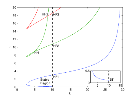
Figure 1: Partial bifurcation sets with parameters in the $k-\tau$ plane. The color lines are Hopf bifurcation curve and the dotted line stands for the fold bifurcation curve.

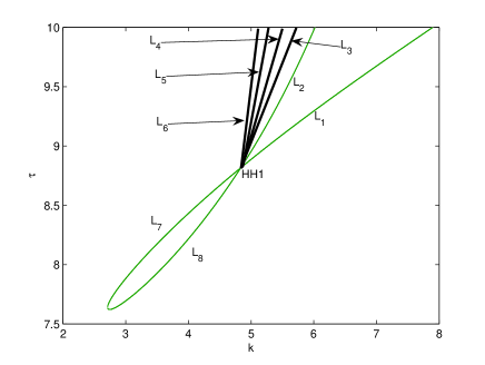
Figure 2: Complete bifurcation sets near HH1.

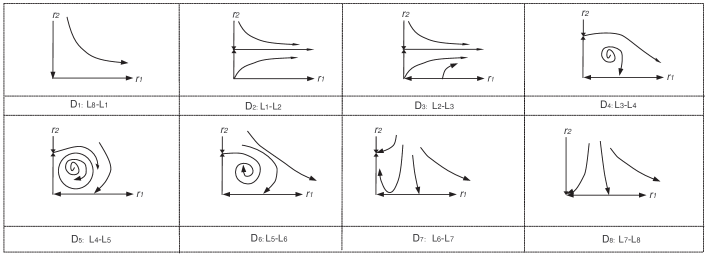
Figure 3: The eight distinct phase portraits near HH1 in $D_{1}$–$D_{8}$. Below every figure, we mark the corresponding region in Figure 2, e.g. the region $D_{1}$ is between $L_{8}$ and $L_{1}$.

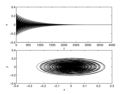
Figure 4: $\alpha_{1}=-0.1$, $\alpha_{2}=-0.08$ in $D_{8}$. The trivial equilibrium of system (24) is stable.

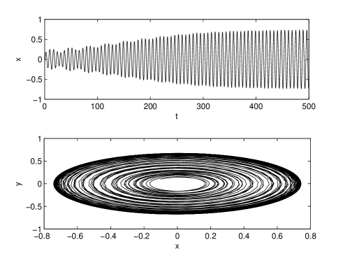
Figure 5: $\alpha_{1}=-0.1$, $\alpha_{2}=0.1$ in $D_{7}$. System (24) has a stable periodic solution in Region $D_{7}$.

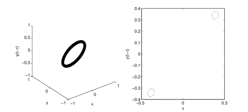
Figure 6: $\alpha_{1}=0.1$, $\alpha_{2}=0.085$ in $D_{6}$. The bifurcated quasi-periodic solution of system (24).

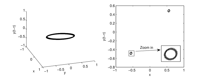
Figure 7: $\alpha_{1}=0.2$, $\alpha_{2}=0.164$ in $D_{5}$. The bifurcated quasi-periodic solution on the three-dimensional torus of system (24) and the corresponding Poincar$\acute{\textrm{e}}$ map on the whole Poincar$\acute{\textrm{e}}$ section $y(t)=0$.

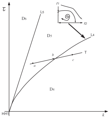
Figure 8: The sketch of the saddle connection bifurcation curve ($L_{4}$) on the three-dimensional torus. (a) $(\alpha_{1},\alpha_{2})=2\times(0.1,0.081)$; (b) $(\alpha_{1},\alpha_{2})=2.4\times(0.1,0.081)$; (c) $(\alpha_{1},\alpha_{2})=2.5\times(0.1,0.081)$.

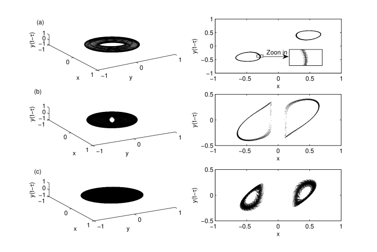
Figure 9: $\alpha_{1}=0.2$, $\alpha_{2}=0.164$. The phase portraits in $x$–$y$–$y(\cdot-\tau)$ space and the corresponding Poincar$\acute{\textrm{e}}$ map on the whole Poincar$\acute{\textrm{e}}$ section $y(t)=0$ when parameters are chosen at (a), (b) and (c) in Figure 8, respectively.

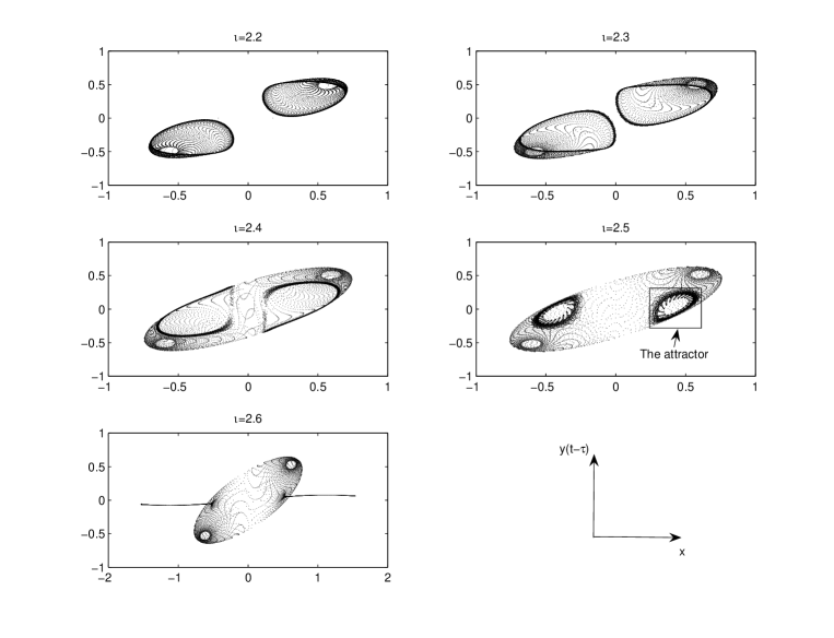
Figure 10: The complete Poincaré maps near the saddle connection.

IV Conclusions

In this paper we mainly study the nonresonant Hopf-Hopf bifurcation in a NFDE with parameters as follows

$$\frac{d}{dt}\left[Dx_{t}-G(x_{t})\right]=L(\alpha)x_{t}+F(\alpha,x_{t})$$ (36)

Following Faria1 ; Faria2 ; Wee ; WangWei1 , we compute the normal form near the bifurcation point. An explicit algorithm is given to calculate the four key variables: $b_{0},~{}c_{0},~{}d_{0}$ and $d_{0}-b_{0}c_{0}$, by which the twelve unfoldings are distinguished. We find that the operator $D$ just changes the method when transforming the NFDE to a abstract ODE and the decomposing of phase space, compared with the normal form derivation for RFDE. All the rest steps of calculations remain almost the same as dealing with a RFDE.

As an illustration of this theory, van der Pol’s equation with extended delay feedback is considered. We give the conditions under which the Hopf-Hopf bifurcation occurs. Detailed dynamics near the origin are obtained by drawing the corresponding bifurcation set. Both theoretical bifurcation set and simulations confirm the existence of stable periodic solutions and stable quasi-periodic solutions. With the guide of the bifurcation sets we also find in van der Pol’s equation a chaotic attractor appears as the three-dimensional torus vanishes via a saddle connection bifurcation.

References

- (1) J. Guckenheimer, P. Holmes, Nonlinear Oscillations, Dynamical Systems, and Bifurcations of Vector Fields, Springer, New York, 1983.
- (2) J. Hale, Ordinary Differential Equations, Wiley, NewYork, 1969.
- (3) S. Wiggins, Introduction to Applied Nonlinear Dynamical Systems and Chaos, Springer, New York, 1980.
- (4) T. Faria, L. Magalhaes, Normal forms for retarded functional differential equation and applications to Bogdanov-Takens singularity, J. Differ. Equations. 122 (1995) 201–224.
- (5) T. Faria, L. Magalhaes, Normal forms for retarded functional differential equation with parameters and applications to Hopf bifurcation, J. Differ. Equations. 122 (1995) 181–200.
- (6) B. Hassard, N.D. Kazarinoff, Y. Wan, Theory and applications of Hopf bifurcation, Cambridge Univ. Press, 1981.
- (7) M. Weedermann, Normal forms for neutral functional differential equations. In: T. Faria, P. Freitas (Eds.), Topics in Functional Differential and Difference Equations, Amer. Math. Soc., Providence, 2001, pp. 361-368.
- (8) M. Weedermann, Hopf bifurcation calculations for scalar neutral delay differential equations, Nonlinearity. 19 (2006) 2091–2102.
- (9) C. Wang, J. Wei, Normal forms for NFDE with parameters and application to the lossless transmission line, Nonlinear Dynam. 52 (2008) 199–206.
- (10) J. Wu, Theory and applications of partial functional differential equations, Springer, New York, 1995.
- (11) J. Hale, S. Lunel, Introduction to Functional Differential Equations, Springer, New York, 1993.
- (12) J. Wei, S. Ruan, Stability and global Hopf bifurcation for neutral differential equations, Acta. Math. Sin. 45 (2002) 94–104.
- (13) J. Wu, H. Xia, Self-sustained oscillations in a ring array of lossless transmission lines, J. Differ. Equations. 124 (1996) 247–278.
- (14) W. Krawcewicz, S. Ma, J. Wu, Multiple slowly oscillating periodic solutions in coupled lossless transmission lines, Nonlinear Anal. RWA. 5 (2004) 309–354.
- (15) Z. Balanov, W. Krawcewicz, H. Ruan, Hopf bifurcation in a symmetric configuration of transmission lines, Nonlinear Anal. RWA. 8 (2007) 1144-1170.
- (16) W. Jiang, Y. Yuan, Bogdanov-Takens singularity in Van der Pol’s oscillator with delayed feedback, Physica D. 227 (2007) 149–161.
- (17) W. Jiang, H. Wang, Hopf-transcritical bifurcation in retarded functional differential equations, Nonlinear Anal. TMA. 73 (2010) 3626–3640.
- (18) H. Wang, W. Jiang, Hopf-pitchfork bifurcation in van der Pol’s oscillator with nonlinear delayed feedback, J. Math. Anal. Appl. 368 (2010) 9–18.
- (19) J. Zhang, W. Li, X. Yan, Multiple bifurcations in a delayed predator Cprey diffusion system with a functional response, Nonlinear Anal. TMA. 11 (2010) 2708–2725.
- (20) S. Ma, Q. Lu, Z. Feng, Double Hopf bifurcation for van der Pol-Duffing oscillator with parametric delay feedback control, J. Math. Anal. Appl. 338 (2008) 993–1007.
- (21) P.Buono, J. Blair, Restrictions and unfolding of double Hopf bifurcation in func- tional differntial equations, J. Differ. Equations, 189 (2003) 234–266.
- (22) K. Pyragas, Control of chaos via extended delay feedback, Phys. Lett. A. 206 (1995) 323–330.
- (23) F. Atay, Van der Pol s oscillator under delayed feedback, J. Sound Vibrat. 218 (1998) 333–339.
- (24) A. Maccari, Vibration control for the primary resonance of the van der Pol oscillator by a time delay state feedback, Int. J. Non-Linear Mech. 38 (2003) 123–131.
- (25) J. Wei, W. Jiang, Stability and bifurcation analysis in Van der Pol’s oscillator with delayed feedback, J. Sound Vibrat. 283 (2005) 801–819.
- (26) S. Wiggins, Application of center manifold theory, Springer, New York, 1981.
- (27) S. -N. Chow, K. Lu, center unstable manifolds, Proc. Roy. Soc. Edinburgh. 108 (1988) 303–320.
- (28) J. Carr, Applications of Centre Manifold Theory, Springer, New York, 1981.
- (29) J. Xu, K. Chung, C. Chan, An efficient method for studying weak resonant double Hopf bifurcation in nonlinear systems with delayed feedbacks, SIAM J. Appl. Dyn. Syst. 6(2007) 29–60.
- (30) P. Battelino1, C. Grebogi, E. Ott, J. Yorke, Chaotic attractors on a 3-torus, and torus break-up, Physica D. 39(1989) 299–314.
- (31) D. Ruelle, F. Takens, On the nature of turbulence, Comm. Math. Phys. 20 (1971) 167–192.
- (32) J.P. Eckmann, Roads to turbulence in dissipative dynamical systems, Rev. Modern Phys. 53 (1981) 643–654.