Is the molecular Berry phase an artifact of the Born-Oppenheimer approximation?

Abstract

We demonstrate that the molecular Berry phase and the corresponding non-analyticity in the electronic Born-Oppenheimer wavefunction is, in general, not a true topological feature of the exact solution of the full electron-nuclear Schrödinger equation. For a numerically exactly solvable model we show that a non-analyticity, and the associated geometric phase, only appear in the limit of infinite nuclear mass, while a perfectly smooth behavior is found for any finite nuclear mass.

Geometric phases are ubiquitous in physics and chemistry, and some of the most fascinating phenomena in condensed matter science such as topological insulators Fu et al. (2007); Hasan and Kane (2010), ferroelectrics Resta (1994); Xiao et al. (2010), the Aharonov-Bohm effect Aharonov and Bohm (1959) as well as conical intersections in molecules Mead (1992); Yarkony (1996); Kendrick (1997); Juanes-Marcos et al. (2005) are closely associated with Berry phases. Geometric phases may arise when the Hamiltonian of a system depends on a set of parameters ${\underline{\bf R}}$. In Berry’s original definition Berry (1984), this parameter set is allowed to change adiabatically, i.e. very slowly in time along a given path $C=\{{\underline{\bf R}}(t^{\prime})|t^{\prime}\in[t_{0},t]\}$ such that the solution of the time-dependent Schrödinger equation (TDSE),

$$i{\frac{\partial}{\partial t}}\Phi_{n}({\underline{\bf r}};t)={\hat{H}}^{BO}({\underline{\bf r}};{\underline{\bf R}}(t))\Phi_{n}({\underline{\bf r}};t),$$ (1)

by virtue of the adiabatic theorem, is given by

$$\Phi_{n}\!({\underline{\bf r}};t)\!=\!e^{-i\!\int^{t}_{t_{0}}\!\!\epsilon^{BO}_{n}\!({\underline{\bf R}}(t^{\prime}))dt^{\prime}}\!e^{-i\gamma_{n}(C)}\Phi^{BO}_{n}\!({\underline{\bf r}};{\underline{\bf R}}(t))$$ (2)

where

$${\hat{H}}^{BO}({\underline{\bf r}};{\underline{\bf R}})\Phi^{BO}_{n}({\underline{\bf r}};{\underline{\bf R}})=\epsilon^{BO}_{n}({\underline{\bf R}})\Phi^{BO}_{n}({\underline{\bf r}};{\underline{\bf R}}).$$ (3)

In Eq. (2), the first exponent is a dynamical phase which appears naturally from the TDSE while the second exponent, $\gamma_{n}(C)$, is given in terms of the Berry connection,

$${\bf A}^{BO}_{\nu,n}({\underline{\bf R}}) =\langle\Phi^{BO}_{n}({\underline{\bf R}})|-i\nabla_{\nu}\Phi^{BO}_{n}({\underline{\bf R}})\rangle_{\underline{\bf r}},$$ (4)

as a line integral along the path $C$

$$\gamma^{BO}_{n}(C) =\int_{C}\sum_{\nu}{\bf A}^{BO}_{\nu,n}({\underline{\bf R}})\cdot d{\bf R}_{\nu}$$

$$=\sum_{\nu}\int_{t_{0}}^{t}\!dt^{\prime}{\bf A}^{BO}_{\nu,n}({\underline{\bf R}}(t^{\prime}))\cdot\frac{d{\bf R}_{\nu}(t^{\prime})}{dt^{\prime}}.$$ (5)

The notation $\langle\cdots\rangle_{\underline{\bf r}}$ indicates integration over ${\underline{\bf r}}$-space only. All quantities in this Letter are in atomic units, and a bold value with underline represents a multi-dimensional vector, i.e. ${\underline{\bf X}}\equiv\{{\bf X}_{\nu}|\nu=1,\cdots\}$. When $C$ becomes a closed loop, ${\mathcal{L}}$, this line integral,

$$\gamma^{BO}_{n}({\mathcal{L}}) =\oint_{{\mathcal{L}}}\sum_{\nu}{\bf A}^{BO}_{\nu,n}({\underline{\bf R}})\cdot d{\underline{\bf R}}_{\nu},$$ (6)

may give a non-vanishing value if the loop encloses a conical intersection (CI). The value of $\gamma_{n}^{BO}({\mathcal{L}})$ does not depend on the shape of ${\mathcal{L}}$ as long as the loop encloses the CI. While the concept displayed in Eqs. (1)-(6) is completely general, i.e. may refer to any Hamiltonian that depends on a set of parameters, ${\underline{\bf R}}$, the specific case the notation in Eqs. (1)-(6) refers to is the molecular Berry phase appearing in the Born-Oppenheimer (BO) approximation. The latter is fundamental to all modern condensed matter theory. It derives from the fact that, in most cases, the nuclei move extremely slowly compared to the electrons. Hence, as a first step, it is reasonable to neglect the nuclear kinetic energy operator in the complete molecular Hamiltonian leading to the so-called BO Hamiltonian,

$${\hat{H}}^{BO}({\underline{\bf r}};{\underline{\bf R}})\!=\!{\hat{T}}_{e}({\underline{\bf r}})\!+\!{\hat{V}}_{ee}({\underline{\bf r}})\!+\!{\hat{V}}_{en}({\underline{\bf r}},{\underline{\bf R}})\!+\!{\hat{V}}_{nn}({\underline{\bf R}}).$$ (7)

Here ${\hat{T}}_{e}$ is the electronic kinetic energy operator, ${\hat{V}}_{ee}({\hat{V}}_{nn})$ is the repulsive electron-electron (nuclear-nuclear) interaction, and ${\hat{V}}_{en}$ is the electron-nuclear Coulomb attraction. The complete molecular wavefunction can then be approximated by the adiabatic ansatz $\Psi^{BO}_{mol}({\underline{\bf r}},{\underline{\bf R}})=\chi^{BO}_{kn}({\underline{\bf R}})\Phi^{BO}_{n}({\underline{\bf r}};{\underline{\bf R}})$ where $\chi^{BO}_{kn}({\underline{\bf R}})$ satisfies the Schrödinger equation

$$\left[\sum_{\nu}\!\!\frac{(-i\nabla_{\nu}\!+\!{\bf A}^{BO}_{\nu,n})^{2}}{2M_{\nu}}\!+\!\tilde{\epsilon}^{BO}_{n}\!({\underline{\bf R}})\right]\!\!\chi^{BO}_{kn}\!({\underline{\bf R}})\!\!=\!\!E_{kn}\!\chi^{BO}_{kn}\!({\underline{\bf R}})$$ (8)

with the generalized BO potential energy surface,

$$\tilde{\epsilon}^{BO}_{n} \!({\underline{\bf R}})\!\!=\langle\Phi^{BO}_{n}({\underline{\bf R}})\!|{\hat{H}}_{BO}({\underline{\bf R}})\!|\Phi^{BO}_{n}\!({\underline{\bf R}})\rangle_{\underline{\bf r}}\!$$

$$+\!\sum_{\nu}\!\!\frac{\langle\nabla_{\nu}\Phi^{BO}_{n}\!({\underline{\bf R}})|\nabla_{\nu}\Phi^{BO}_{n}\!({\underline{\bf R}})\rangle_{\underline{\bf r}}}{2M_{\nu}}\!-\!\sum_{\nu}\!\!\frac{{\bf A}^{BO}_{\nu,n}\!({\underline{\bf R}})^{2}}{2M_{\nu}}.$$ (9)

Here $M_{\nu}$ is the mass of the $\nu$-th nucleus. After the seminal work of Mead and Truhlar Mead and Truhlar (1979), a lot of attention has been devoted to the molecular Berry phase associated with the vector potential, Eq. (4) Wilczek and Shapere (1989); Domcke et al. (2004). An essential aspect of the molecular geometric phase is that it always appears in the presence of some kind of non-analyticity in the ${\underline{\bf R}}$-dependence of $\epsilon^{BO}_{n}({\underline{\bf R}})$ and $\Phi^{BO}_{n}({\underline{\bf r}};{\underline{\bf R}})$. Similar to Cauchy’s theorem in complex analysis, where a loop integral in the complex plane picks up a phase if the loop encloses a pole, the line integral in Eq. (6) may pick up a Berry phase if the loop encloses a CI of BO surfaces. Clearly, in the case of the molecular Berry phase, the parametric dependence of the Hamiltonian in Eq. (3) is the result of an approximation, the BO approximation. In the full molecular Hamiltonian, ${\underline{\bf R}}$ is a dynamical variable. The objective of this Letter is to investigate whether this very specific topological feature, this non-analyticity in the ${\underline{\bf R}}$-dependence of the wavefunction, only occurs within the BO approximation or whether it may survive as a feature of the full molecular wavefunction $\Psi_{mol}({\underline{\bf r}},{\underline{\bf R}})$, i.e. as a true feature of nature. To investigate this question, we employ the recently derived framework of exact factorization of $\Psi_{mol}({\underline{\bf r}},{\underline{\bf R}})$  Gidopoulos and Gross (ress); Hunter (1975); Abedi et al. (2010, 2012, 2013). This formulation lends itself as a natural framework because it leads to a Berry-type vector potential but without invoking the BO approximation.

Within this formulation, $\Psi^{N}_{mol}({\underline{\bf r}},{\underline{\bf R}})$, the exact $N$-th eigenstate of the full molecular Schrödinger equation ${\hat{H}}({\underline{\bf r}},{\underline{\bf R}})\Psi^{N}_{mol}({\underline{\bf r}},{\underline{\bf R}})=E_{N}\Psi^{N}_{mol}({\underline{\bf r}},{\underline{\bf R}})$, can be factorized as a single product $\Psi^{N}_{mol}({\underline{\bf r}},{\underline{\bf R}})\!\!=\!\!\chi_{N}({\underline{\bf R}})\Phi_{N}({\underline{\bf r}};{\underline{\bf R}})$, where $\Phi_{N}({\underline{\bf r}};{\underline{\bf R}})$ satisfies the partial normalization condition, $\int\!\!d{\underline{\bf r}}|\Phi_{N}({\underline{\bf r}};{\underline{\bf R}})|^{2}=1$. The equations which $\Phi_{N}({\underline{\bf r}};{\underline{\bf R}})$ and $\chi_{N}({\underline{\bf R}})$ satisfy are

$$\left[\!{\hat{H}}^{BO}\!({\underline{\bf r}};{\underline{\bf R}})\!+\!{\hat{U}}_{en}\!({\underline{\bf r}},{\underline{\bf R}})\!\right]\!\!\Phi_{N}\!({\underline{\bf r}};{\underline{\bf R}})\!=\!\epsilon^{ex}_{N}\!({\underline{\bf R}})\Phi_{N}\!({\underline{\bf r}};{\underline{\bf R}})$$ (10)

$$\left[\sum_{\nu}\!\!\frac{(-i\nabla_{\nu}+{\bf A}^{ex}_{\nu,N})^{2}}{2M_{\nu}}\!+\!\epsilon^{ex}_{N}({\underline{\bf R}})\right]\!\chi_{N}\!({\underline{\bf R}})\!\!=\!\!E_{N}\chi_{N}\!({\underline{\bf R}})$$ (11)

where ${\hat{U}}_{en}$ is an electron-nucleus coupling operator given by

$${\hat{U}}_{en}({\underline{\bf r}},{\underline{\bf R}}) =\sum_{\nu}\frac{1}{M_{\nu}}\left[\frac{(-i\nabla_{\nu}-{\bf A}^{ex}_{\nu,N})^{2}}{2}\right.$$

$$\left.+\left(\frac{-i\nabla_{\nu}\chi_{N}}{\chi_{N}}\!+\!{\bf A}^{ex}_{\nu,N}\right)\!\cdot\!(-i\nabla_{\nu}\!-\!{\bf A}^{ex}_{\nu,N})\right].$$ (12)

$\epsilon^{ex}_{N}({\underline{\bf R}})$ is defined as

$$\epsilon^{ex}_{N} \!({\underline{\bf R}})\!\!=\langle\Phi_{N}({\underline{\bf R}})|{\hat{H}}_{BO}({\underline{\bf R}})|\Phi_{N}({\underline{\bf R}})\rangle_{\underline{\bf r}}\!$$

$$+\!\sum_{\nu}\!\!\frac{\langle\nabla_{\nu}\Phi_{N}({\underline{\bf R}})|\nabla_{\nu}\Phi_{N}({\underline{\bf R}})\rangle_{\underline{\bf r}}}{2M_{\nu}}\!-\!\sum_{\nu}\!\!\frac{{\bf A}^{ex}_{\nu,N}({\underline{\bf R}})^{2}}{2M_{\nu}},$$ (13)

and

$${\bf A}^{ex}_{\nu,N}({\underline{\bf R}})=\langle\Phi_{N}({\underline{\bf R}})|-i\nabla_{\nu}\Phi_{N}({\underline{\bf R}})\rangle_{\underline{\bf r}}.$$ (14)

Because $\epsilon^{ex}_{N}({\underline{\bf R}})$ and ${\underline{\bf A}}^{ex}_{N}({\underline{\bf R}})$ yield the exact many-body nuclear density, $|\chi_{N}({\underline{\bf R}})|^{2}\!=\!\int d{\underline{\bf r}}|\Psi^{N}_{mol}({\underline{\bf r}},{\underline{\bf R}})|^{2}$, and the exact many-body nuclear current density, $1/M_{\nu}\!\left(\operatorname{Im}\!\left[\chi_{N}^{*}\nabla_{\nu}\chi_{N}\right]\!+\!|\chi_{N}|^{2}\!{\bf A}^{ex}_{\nu,N}\right)\!=\!1/M_{\nu}\!\left(\operatorname{Im}\!\!\int\!\!d{\underline{\bf r}}\Psi^{N*}_{mol}\nabla_{\nu}\Psi^{N}_{mol}\right)$, we can call $\epsilon^{ex}_{N}({\underline{\bf R}})$ and ${\underline{\bf A}}^{ex}_{N}({\underline{\bf R}})$ the exact scalar potential and the exact vector potential. They are unique up to gauge transformations, $\chi_{N}({\underline{\bf R}})\rightarrow\chi_{N}({\underline{\bf R}})e^{iS({\underline{\bf R}})}$ and $\Phi_{N}({\underline{\bf R}})\rightarrow\Phi_{N}({\underline{\bf R}})e^{-iS({\underline{\bf R}})}$ Abedi et al. (2010, 2012).

Both the exact molecular wavefunction $\Psi^{N}_{mol}({\underline{\bf r}},{\underline{\bf R}})\!=\!\chi_{N}\!({\underline{\bf R}})\Phi_{N}({\underline{\bf r}};{\underline{\bf R}})$ and the adiabatic approximation $\Psi^{BO}_{mol}\!({\underline{\bf r}},{\underline{\bf R}})\!=\!\chi^{BO}_{kn}\!({\underline{\bf R}})\Phi^{BO}_{n}\!({\underline{\bf r}};{\underline{\bf R}})$ are given in terms of a single product of a nuclear and an electronic wavefunction where the latter satisfies the partial normalization condition $\int\!|\Phi({\underline{\bf r}};{\underline{\bf R}})|^{2}d{\underline{\bf r}}\!=\!1$ for each nuclear configuration ${\underline{\bf R}}$. Both in the exact case and in the adiabatic approximation, the nuclear factor satisfies a standard Schrödinger equation (Eqs. (11) and (8), respectively) with a vector potential (Eqs. (14) and (4), respectively) and a scalar potential (Eqs. (Is the molecular Berry phase an artifact of the Born-Oppenheimer approximation?) and (Is the molecular Berry phase an artifact of the Born-Oppenheimer approximation?), respectively) that formally follow the same expression. In particular, the vector potential is defined as a Berry connection in both cases. The only difference is that in the adiabatic approximation the Berry connection ${\underline{\bf A}}^{BO}_{n}({\underline{\bf R}})$, Eq. (4), and the BO potential energy surfaces $\tilde{\epsilon}^{BO}_{n}({\underline{\bf R}})$, Eq. (Is the molecular Berry phase an artifact of the Born-Oppenheimer approximation?), are evaluated from the BO electronic wavefunction $\Phi^{BO}_{n}({\underline{\bf r}};{\underline{\bf R}})$ and while the exact Berry connection ${\underline{\bf A}}^{ex}_{N}({\underline{\bf R}})$, Eq. (14), and the exact potential energy surfaces $\epsilon^{ex}_{N}({\underline{\bf R}})$, Eq. (Is the molecular Berry phase an artifact of the Born-Oppenheimer approximation?), are evaluated with the exact electronic wavefunction coming from Eq. (10). In this sense ${\underline{\bf A}}^{ex}_{N}({\underline{\bf R}})$ represents a feature of the exact molecular wavefunction. Can this exact Berry connection have the fascinating topological structure that gives rise to a non-vanishing Berry phase? In other words, is the geometric phase found within the adiabatic approximation a true feature of nature, or is it merely an “artifact” of the BO approximation?

This is the question we are going to address in the following by studying a 2-dimensional model system which, in the BO approximation, has CIs leading to a Berry phase, and which, at the same time, is simple enough to allow for a numerically exact solution.

The system consists of three ions and an electron. Two of the ions are fixed at $(\pm L/2,0)$, and the third ion as well as the electron are allowed to move in 2-dimensional space. Representing the positions of the moving ion and the electron as ${\bf R}=(X,Y)$ and ${\bf r}=(x,y)$, respectively, the full Hamiltonian is

$${\hat{H}}({\bf r},{\bf R})= -\frac{1}{2M}\nabla_{\bf R}^{2}-\frac{1}{2}\nabla_{\bf r}^{2}+V_{en}(|{\bf r}-(\frac{L}{2},0)|)$$

$$+V_{en}(|{\bf r}-(-\frac{L}{2},0)|)+V_{en}(|{\bf r}-{\bf R}|)$$

$$+V_{nn}(|{\bf R}-(\frac{L}{2},0)|)+V_{nn}(|{\bf R}-(-\frac{L}{2},0)|)$$

$$+V_{nn}(L)+(R/R_{0})^{4}$$ (15)

where the first two terms are the kinetic energy operators for the moving ion and the electron, respectively, and the electron-nucleus interaction potential, $V_{en}(x)=-1/\sqrt{a+x^{2}}$, and the nucleus-nucleus interaction potential, $W_{nn}(x)=1/\sqrt{b+x^{2}}$, are represented as soft Coulomb potentials while the last term is added to make the system bound. Here, the origin is set as the center of the two fixed ions. We choose parameters $a$, $b$, $R_{0}$ and $L$ as 0.5, 10.0, 3.5 and $4\sqrt{3}/5$, respectively. Since the interaction potentials for the three ions are identical, we can expect that symmetry-induced degenerate states exist at equilateral positions ${\bf R}^{\pm}_{eq}\!\!=\!\!(0,\pm Y_{eq})$ where $Y_{eq}\!\!=\!\!\sqrt{3}/2\cdot L=1.2$ with $D_{3h}$ point group symmetry.

In FIG. 1, we present the first and second excited BO surfaces, $\epsilon^{BO}_{1}({\bf R})$ and $\epsilon^{BO}_{2}({\bf R})$, respectively, with the corresponding real-valued BO electronic wavefunctions $\Phi^{BO}_{1,2}({\bf r};{\bf R})$, which are numerical eigenstates of the BO Hamiltonian not . Indeed, we can confirm the degeneracy between the energy levels $\epsilon^{BO}_{1}$ and $\epsilon^{BO}_{2}$ at ${\bf R}^{\pm}_{eq}$ where the energy is -0.286. (Since the $s$-orbital-like ground BO electronic state is not related to CIs, we focus only on $\Phi^{BO}_{1,2}$.) To visualize possible non-analyticities in the wavefunction $\Phi^{BO}_{1,2}({\bf r};{\bf R})$ with respect to ${\bf R}$, we investigate the 2-dimensional vector field $\int{\bf r}\Phi({\bf r};{\bf R})d{\bf r}$ whose direction in space represents the “polarization of the wavefunction”: A $p$-orbital-like electronic wavefunction, $\Phi({\bf r};{\bf R})$, can be represented as a vector pointing from the region of negative values of $\Phi({\bf r};{\bf R})$ to the region of positive values of $\Phi({\bf r};{\bf R})$ in ${\bf r}$-space as depicted in FIG. 1(b). The discontinuities of $\Phi({\bf r};{\bf R})$ appearing in ${\bf R}$-space can then be seen as abrupt changes in the direction of the vectors. We find that a discontinuous phase change occurs across the lines $L_{1,2}$ for $\Phi^{BO}_{1,2}$, respectively, where $L_{1}\!\!=\!\!\{(X,Y)|X\!\!=\!\!0,|Y|\!\!>\!\!Y_{eq}\}$ and $L_{2}\!\!=\!\!\{(X,Y)|X\!\!=\!\!0,|Y|\!\!<\!\!Y_{eq}\}$ (see red vectors in the lower panels of FIG. 1). Along these lines the sign of the $p$-orbital-like electronic wavefunctions, $\Phi^{BO}_{1,2}$, suddenly changes. This leads to a non-zero Berry phase ($\gamma_{n}({\mathcal{L}})=\pi$) if the closed path, ${\mathcal{L}}$, crosses $L_{1}$ or $L_{2}$.

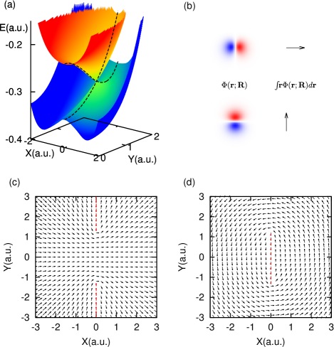
Figure 1: (a) The first (blueish) and second (reddish) excited BO potential energy surfaces, (b) the vector field representation for $p$-orbital-like wavefunctions at a certain ${\bf R}$, and the BO electronic wavefunctions in the vector field representation for the first excited BO state (c) and the second excited BO state (d). The phase changes discontinuously across the line of red vectors ($L_{1}$ and $L_{2}$ in text).

In the exact decomposition framework, there is one potential energy surface for each exact eigenstate, $\Psi^{N}_{mol}({\bf r},{\bf R})$, of the full Hamiltonian, ${\hat{H}}({\bf r},{\bf R})$. Here, we aim at investigating the behavior of the exact potential energy surfaces in the region at and around the points of CIs. To this end, we first calculate the eigenstates of the complete system up to a certain energy, well above the CIs involving the first and second excited BO potential energy surfaces. From the computed $\Psi^{N}_{mol}({\bf r},{\bf R})$, we calculate the exact nuclear wavefunction in a specific gauge as, $\chi_{N}({\bf R})=\sqrt{\int\!\!d{\bf r}|\Psi^{N}_{mol}\!({\bf r},{\bf R})|^{2}}$, and obtain the corresponding exact electronic wavefunction, $\Phi_{N}({\bf r};{\underline{\bf R}})=\Psi^{N}_{mol}({\bf r},{\bf R})/\chi_{N}({\bf R})$. Then, for the subset of the exact electronic wavefunctions, $\Phi_{N}({\bf r};{\underline{\bf R}})$, that exhibit $p$-orbital-like behavior similar to $\Phi^{BO}_{1}({\bf r};{\bf R})$ or $\Phi^{BO}_{2}({\bf r};{\bf R})$, we choose the energetically lowest two eigenstates, denoted as A and B, and calculate the exact potential energy surfaces $\epsilon^{ex}_{A}({\bf R})$ and $\epsilon^{ex}_{B}({\bf R})$ from Eq. (Is the molecular Berry phase an artifact of the Born-Oppenheimer approximation?). In FIG. 2, we have plotted $|\chi_{N}({\bf R})|^{2}$, $\int{\bf r}\Phi_{N}({\bf r};{\underline{\bf R}})d{\bf r}$ and $\epsilon^{ex}_{N}({\bf R})$ ($N\!=\!A,B$) for a nuclear mass of $M\!\!=\!\!10.0$. The eigenenergies of $\Psi^{A,B}_{mol}$ are -0.282 and -0.201, respectively. As it is seen in FIG. 2, for these exact eigenstates, $\chi_{N}({\bf R}^{\pm}_{eq})\neq 0$, and $\Phi_{N}({\bf r};{\underline{\bf R}})$ do not show any abrupt phase changes or singularities. Therefore, $\epsilon^{ex}_{A}({\bf R})$ and $\epsilon^{ex}_{B}({\bf R})$ show a smooth “diabatic” form connecting $\epsilon^{BO}_{1}$ and $\epsilon^{BO}_{2}$ continuously along the $Y$-axis through the points where, in the BO case, are CIs. Consequently, the exact geometric phase $\gamma^{ex}_{N}({\mathcal{L}})=\oint_{\mathcal{L}}{\bf A}^{ex}_{N}({\bf R}^{\prime})\cdot d{\bf R}^{\prime}$ is zero since there is no singular point in $\Phi_{N}({\bf r};{\underline{\bf R}})$ in this case.

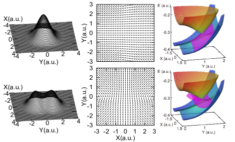
Figure 2: The factorized nuclear densities (left), the corresponding electronic wavefunctions represented by the vector fields $\int\!{\bf r}\Phi_{N}({\bf r};{\underline{\bf R}})d{\bf r}$ (middle) and the potential energy surfaces (right) for the selected full wavefunctions $\Psi^{A}_{mol}$ and $\Psi^{B}_{mol}$ (from top to bottom) with $M=10.0$. The blueish and reddish surfaces are the first and second excited BO potential energy surfaces, respectively, while the pink surfaces are the exact potential energy surfaces near ${\bf R}^{+}_{eq}$.

In the following we investigate how $\Phi_{A}({\bf r};{\underline{\bf R}})$, $|\chi_{A}({\bf R})|^{2}$ and $\epsilon^{ex}_{A}({\bf R})$ evolve as $M$ increases ($M$=1,10,20, and 50) to reach the adiabatic limit ($M\rightarrow\infty$) which is accompanied by a Berry phase. In FIG. 3, we show how the exact electronic wavefunction $\Phi_{A}({\underline{\bf r}};{\underline{\bf R}})$ transforms into $\Phi^{BO}_{1}$ with increasing nuclear mass. For $M\!=\!1$, a set of vectors representing the vector field shows a mainstream simply from left to right. As $M$ increases, however, the mainstream begins to show parabolic behavior, and the curvature of the parabola increases gradually. Compared to $\Phi^{BO}_{1}$ in FIG. 1, we can interpret the discontinuity along $L_{1}$ as coming from the infinite-curvature limit due to the limit $M\rightarrow\infty$. In FIG. 4, we also show $|\chi_{A}|^{2}$ and $|\epsilon^{ex}_{A}-\epsilon^{BO}_{1}|$ for various $M$’s. As $M$ increases, $|\chi_{A}|^{2}$ gets localized on the double-minima of $\epsilon^{ex}_{A}$ and also gets narrower, showing two distinctive humps. For $\epsilon^{ex}_{A}$, the green region around $L_{1}$ shrinks as $M$ increases, which means $\epsilon^{ex}_{A}$ gets closer to $\epsilon^{BO}_{1}$, but maintaining the diabatic behavior along the $Y$-axis. This enables us to deduce that $\epsilon^{ex}_{A}$ in the limit $M\!\!\rightarrow\!\!\infty$ lies on top of the BO potential energy surface $\epsilon^{BO}_{1}$ except for the line $L_{1}$. Since the actual nuclear mass in the real world is finite, there is no discontinuity of the electronic wavefunction implying that the exact geometric phase is zero.

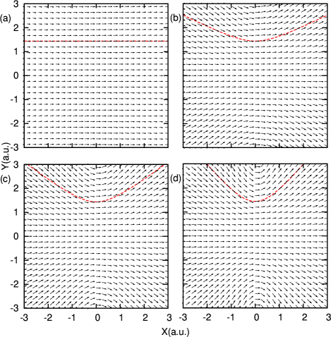
Figure 3: The vector $\int{\bf r}\Phi_{A}({\bf r};{\bf R})d{\bf r}$ is plotted for various ionic masses, $M$. The values of $M$ for th panels (a), (b), (c) and (d) are 1.0, 10.0, 20.0 and 50.0, respectively. The dashed red line indicates, as guide for the eye, the change of curvature as the ionic mass increases.

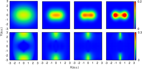
Figure 4: The factorized nuclear densities (first low), and the difference between the exact potential energy surface and the 1st excited BO potential energy surface ($\epsilon^{ex}_{A}-\epsilon^{BO}_{1}$) (second row) for various nuclear masses (M=1.0,10.0,20.0, and 50.0 from left to right).

To summarize, we have investigated whether the specific non-analyticity in $\Phi^{BO}_{n}({\underline{\bf r}};{\underline{\bf R}})$ that leads to a non-trivial geometric phase in the BO approximation is a true topological feature of the full electron-nuclear wavefunction. To shed light on this question, we have studied a numerically exactly solvable model system in 2 dimensions that exhibits non-trivial Berry phases in the BO limit. Employing the exact factorization of the full molecular wavefunction Gidopoulos and Gross (ress); Hunter (1975); Abedi et al. (2010, 2012, 2013) we identify and calculate the exact electronic wavefunctions $\Phi_{N}({\underline{\bf r}};{\underline{\bf R}})$ which, in the limit of infinite nuclear mass $M$, reduce to the BO electronic wavefunctions $\Phi^{BO}_{n}({\underline{\bf r}};{\underline{\bf R}})$. We find that the exact electronic wavefunctions $\Phi_{N}({\underline{\bf r}};{\underline{\bf R}})$ are perfectly smooth for any finite value of the nuclear mass. Consequently the geometric phase associated with the vector potential ${\bf A}^{ex}_{\nu,N}({\underline{\bf R}})=-i\int\Phi^{*}_{N}({\underline{\bf r}};{\underline{\bf R}})\nabla_{\nu}\Phi_{N}({\underline{\bf r}};{\underline{\bf R}})d{\underline{\bf r}}$ vanishes. Only in the limit $M\rightarrow\infty$ (the BO limit) a discontinuous phase change appears which leads to a non-trivial Berry phase. In this sense, the molecular Berry phase can be viewed as an artifact of the BO approximation. The specific topological feature, the non-analyticity of the BO electronic wavefunction leading to the BO geometric phase is not a feature of the true molecular wavefunction. Whether or not this statement holds true for all molecules and solids is currently not known. One easily verifies that nodes at specific nuclear configurations ${\underline{\bf R}}_{0}$ in the exact molecular wavefunction, $\Psi^{N}_{mol}({\underline{\bf r}},{\underline{\bf R}})$, directly lead to singularities in the exact vector potential ${\underline{\bf A}}^{ex}_{N}({\underline{\bf R}})$. Whether such singularities can produce non-trivial Berry phases remains the subject of future research.

We acknowledte partial support from the Deutsche Forschungsgemeinschaft (SFB 762), the European Commission (FP7-NMP-CRONOS), NRF (National Honor Scientist Program: 2010-0020414) and KISTI (KSC-2011-G3-02)

References

Fu et al. (2007)L. Fu, C. L. Kane, and E. J. Mele, Phys. Rev. Lett. 98, 106803 (2007).
Hasan and Kane (2010)M. Z. Hasan and C. L. Kane, Rev.
Mod. Phys. 82, 3045
(2010).
Kendrick (1997)B. Kendrick, Phys. Rev. Lett. 79, 2431 (1997).
Juanes-Marcos et al. (2005)J. C. Juanes-Marcos, S. C. Althorpe, and E. Wrede, Science 309, 1227
(2005).
Berry (1984)M. V. Berry, Proc.
R. Soc. London, Ser. A 392, 45 (1984).
Mead and Truhlar (1979)C. Mead and D. Truhlar, J. Chem. Phys. 70, 2284 (1979).
Wilczek and Shapere (1989)F. Wilczek and A. Shapere, Geometric phases in
physics, Vol. 5 (World
Scientific, 1989).
Domcke et al. (2004)W. Domcke, D. Yarkony, and H. Köppel, Conical Intersections: Electronic
Structure, Dynamics & Spectroscopy, Vol. 15 (World Scientific Publishing Company Incorporated, 2004).
Gidopoulos and Gross (ress)N. I. Gidopoulos and E. K. U. Gross, arXiv
preprint cond-mat/0502433, Phil. Trans. R. Soc. A (2014, in press).
(19)We use a numerical grid method with grid
spacing 0.12 a.u. and 0.3 a.u. for the nuclear and electronic space,
respectively. The number of grid points are 101 and 81 for each axis in
nuclear and electronic space, respectively.