Light-front holography
and the light-front coupled-cluster method

Abstract

We summarize the light-front coupled-cluster (LFCC) method for the solution of field-theoretic bound-state eigenvalue problems and indicate the connection with light-front holographic QCD. This includes a sample application of the LFCC method and leads to a relativistic quark model for mesons that adds longitudinal dynamics to the usual transverse light-front holographic Schrödinger equation.

I Introduction

In order to compute hadronic light-front wave functions, we need a method by which the light-front QCD Hamiltonian eigenvalue problem can be solved nonperturbatively. The standard approach is to expand the eigenstate in a truncated Fock basis, with the wave functions as the expansion coefficients, and solve the resulting integral equations for these wave functions. The light-front coupled-cluster (LFCC) method LFCC follows this path, except that the Fock basis is not truncated; instead, the wave functions for higher Fock states are restricted to being determined from the wave functions for the lowest states through functions that satisfy nonlinear integral equations. In the lowest Fock sector, designated the valence sector, there is an eigenvalue problem for an effective LFCC Hamiltonian that approximates the effects of higher Fock states. It is this restricted eigenvalue problem that is related to the light-front holographic eigenvalue problem holographicQCD , which is usually presented in the form of a transverse light-front Schrödinger equation for massless quarks. We extend light-front holography to include a longitudinal equation and masses for quarks LongWF .

The truncation of the Fock basis should be avoided, because it causes uncanceled divergences. The analog in Feynman perturbation theory is to separate diagrams into time-ordered diagrams and discard time orderings that include intermediate states with more particles than some finite limit. This destroys covariance, disrupts regularization, and induces spectator dependence for subdiagrams. For example, the Ward identity of gauge theories is destroyed by truncation, as illustrated in Fig. 1. In the nonperturbative case, this happens not just to some finite order in the coupling but to all orders. The LFCC method is designed to avoid this sort of complication.

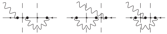
Figure 1: One-loop diagrams contributing to the Ward identity. When only one intermediate photon is allowed, only one diagram survives and the Ward identity fails.

As its name implies, the LFCC method is for light-front quantized Hamiltonians. We define light-front coordinates Dirac as the light-front time $x^{+}=t+z$ and space $\underline{x}=\left(x^{-}\equiv t-z,\vec{x}_{\perp}=(x,y)\right)$. The corresponding light-front energy and momentum are $p^{-}=E-p_{z}$ and $\underline{p}=\left(p^{+}\equiv E+p_{z},\vec{p}_{\perp}=(p_{x},p_{y})\right)$. These imply that the mass-shell condition $p^{2}=m^{2}$ becomes $p^{-}=\frac{m^{2}+p_{\perp}^{2}}{p^{+}}$, and the mass eigenvalue problem is

$${\cal P}^{-}|\underline{P}\rangle=\frac{M^{2}+P_{\perp}^{2}}{P^{+}}|\underline{P}\rangle,\;\;\;\;\underline{\cal P}|\underline{P}\rangle=\underline{P}|\underline{P}\rangle.$$ (1)

Light-front coordinates have several advantages DLCQreviews . There are no spurious vacuum contributions to eigenstates, because $p^{+}>0$ for all particles, which prevents particle production from the vacuum without violation of momentum conservation. This permits well-defined Fock-state wave functions with no spurious vacuum contributions. Also, there is a boost-invariant separation of internal and external momenta, so that wave functions can depend on internal momenta only, which are usually taken to be the longitudinal momentum fractions $x_{i}\equiv p_{i}^{+}/P^{+}$ and relative transverse momenta $\vec{k}_{i\perp}\equiv\vec{p}_{i\perp}-x_{i}\vec{P}_{\perp}$.

II Light-front coupled-cluster method

The LFCC method solves the Hamiltonian eigenvalue problem by first writing the eigenstate as $|\psi\rangle=\sqrt{Z}e^{T}|\phi\rangle$, where $|\phi\rangle$ is the valence state, with normalization $\langle\phi^{\prime}|\phi\rangle=\delta(\underline{P}^{\prime}-\underline{P})$, and $T$ is an operator that increases particle number. The overall normalization is set by $Z$, such that $\langle\psi^{\prime}|\psi\rangle=\delta(\underline{P}^{\prime}-\underline{P})$. $T$ conserves all quantum numbers, including $J_{z}$, light-front momentum $\underline{P}$, and charge. Because $p^{+}$ is positive, $T$ must include annihilation, and powers of $T$ include contractions. The LFCC effective Hamiltonian is constructed as $\overline{{\cal P}-}=e^{-T}{\cal P}^{-}e^{T}$. Then, with $P_{v}$ the projection onto the valence Fock sector, we have the coupled system

$$P_{v}\overline{{\cal P}^{-}}|\phi\rangle=\frac{M^{2}+P_{\perp}^{2}}{P^{+}}|\phi\rangle,\;\;\;\;(1-P_{v})\overline{{\cal P}^{-}}|\phi\rangle=0.$$ (2)

Formulated in this fashion, the eigenvalue problem is still exact but also still infinite in size, because there are, in general, infinitely many terms in $T$. To have a finite problem, but without truncation of the Fock basis, we truncate $T$ and $1-P_{v}$. The simplest truncation of $T$ is to include single-particle emission, such as a gluon from a quark; the corresponding truncation of $1-P_{v}$ would be to project onto Fock states with one more gluon than the valence state. The truncation of $1-P_{v}$ then provides just enough equations to solve for the emission vertex function contained in $T$. The truncations can be systematically relaxed, by expanding the number of particles created by $T$ and the range of Fock states used for projections.

The mathematics of the LFCC method have their origin in the nonrelativistic many-body coupled-cluster method CCorigin , developed in nuclear physics and quantum chemistry CCreviews . It was first applied to the many-electron problem in molecules by Čižek Cizek . The Hamiltonian eigenstate is formed as $e^{T}|\phi\rangle$, where $|\phi\rangle$ is a product of single-particle states and where terms in $T$ annihilate states in $|\phi\rangle$ and create excited states, to build in correlations. The operator $T$ is then truncated at some number of excitations; however, the number of particles does not change. There are also some applications to quantum field theory in equal-time quantization CC-QFT .

Once the LFCC eigenvalue problem has been solved, the solution can be used to compute observables, such as form factors. For a dressed fermion, the Dirac and Pauli form factors can be computed from a matrix element of the current $J^{+}=\overline{\psi}\gamma^{+}\psi$, which couples to a photon of momentum $q$. The matrix element is generally BrodskyDrell

$$\langle\psi^{\sigma}(\underline{P}+\underline{q})|16\pi^{3}J^{+}(0)|\psi^{\pm}(\underline{P})\rangle=2\delta_{\sigma\pm}F_{1}(q^{2})\pm\frac{q^{1}\pm iq^{2}}{M}\delta_{\sigma\mp}F_{2}(q^{2}),$$ (3)

with $F_{1}$ and $F_{2}$ the Dirac and Pauli form factors. Thus, we need to be able to compute matrix elements.

As an example of how a matrix element can be computed, we consider the expectation value for an operator $\hat{O}$, which in the LFCC method would be expressed as

$$\langle\hat{O}\rangle=\frac{\langle\phi|e^{T^{\dagger}}\hat{O}e^{T}|\phi\rangle}{\langle\phi|e^{T^{\dagger}}e^{T}|\phi\rangle}.$$ (4)

Direct computation would require an infinite sum over the untruncated Fock basis. Instead, we define $\overline{O}=e^{-T}\hat{O}e^{T}$ and $\langle\tilde{\psi}|=\langle\phi|\frac{e^{T^{\dagger}}e^{T}}{\langle\phi|e^{T^{\dagger}}e^{T}|\phi\rangle}$, so that $\langle\hat{O}\rangle=\langle\tilde{\psi}|\overline{O}|\phi\rangle$ and $\langle\tilde{\psi}^{\prime}|\phi\rangle=\langle\phi^{\prime}|\frac{e^{T^{\dagger}}e^{T}}{\langle\phi|e^{T^{\dagger}}e^{T}|\phi\rangle}|\phi\rangle=\delta(\underline{P}^{\prime}-\underline{P})$. The effective operator $\overline{O}$ is computed from the Baker–Hausdorff expansion, $\overline{O}=\hat{O}+[\hat{O},T]+\frac{1}{2}[[\hat{O},T],T]+\cdots$. The bra $\langle\tilde{\psi}|$ is a left eigenvector of $\overline{{\cal P}^{-}}$, because the following holds:

$$\langle\tilde{\psi}|\overline{{\cal P}^{-}}=\langle\phi|\frac{e^{T^{\dagger}}{\cal P}^{-}e^{T}}{\langle\phi|e^{T^{\dagger}}e^{T}|\phi\rangle}=\langle\phi|\overline{{\cal P}^{-}}^{\dagger}\frac{e^{T^{\dagger}}e^{T}}{\langle\phi|e^{T^{\dagger}}e^{T}|\phi\rangle}=\frac{M^{2}+P_{\perp}^{2}}{P^{+}}\langle\tilde{\psi}|.$$ (5)

With this technique, the Dirac form factor is approximated by the matrix element

$$F_{1}(q^{2})=8\pi^{3}\langle\widetilde{\psi}^{\pm}(\underline{P}+\underline{q})|\overline{J^{+}(0)}|\phi^{\pm}(\underline{P})\rangle,$$ (6)

with $\overline{J^{+}(0)}=J^{+}(0)+[J^{+}(0),T]+\cdots$.

III Sample LFCC application

As an example of the use of the LFCC method LFCC , we consider a soluble model, a light-front analog model of the Greenberg–Schweber model Greenberg . In this model, a heavy fermionic source emits and absorbs bosons without changing its spin, and we solve for the fermionic eigenstate dressed by a cloud of bosons. A graphical representation of the light-front Hamiltonian ${\cal P}^{-}$ is given in Fig. 2.

Figure 2: Graphical representation of the light-front Hamiltonian ${\cal P}^{-}$ for the soluble model discussed in Sec. III. A cross represents a kinetic energy contribution. Lines on the right represent annihilation operators; lines on left, creation operators. Solid lines are for the fermion, and dashed lines, for the boson.

The model is not fully covariant; in particular, states are all limited to having a fixed total transverse momentum. This hides some of the power of the LFCC method, but is sufficient to show how the method can be applied. Details can be found in Ref. LFCC .

Here we compare the LFCC method with a traditional truncated-Fock-space approach. The Fock-state expansion of the eigenstate is represented in Fig. 3(a). For the LFCC method, we take the valence state to be the bare fermion. The resulting LFCC form of the eigenstate is represented in Fig. 3(b).

(a)

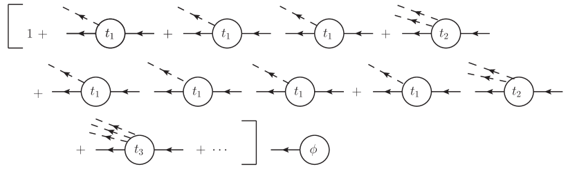
(b)

Figure 3: The model eigenstate as (a) Fock-state expansion and (b) LFCC construction. Bosons are represented by dashed lines, and the fermion by a solid line. The $\psi_{n}$ are the Fock-state wave functions; the $t_{n}$ are the functions that determine the structure of the $T$ operator, by setting the momentum distribution of the $n$ created bosons. The bare fermion state is represented by $\psi_{0}$ in (a) and by $\phi$ in (b). The line to the right of each $t_{n}$ bubble represents a fermion annihilation operator that is contracted with a creation operator in the bare fermion state or the next $t_{n}$ vertex.

We truncate the $T$ operator to include only single boson emission, which corresponds to the terms with $t_{1}$ in Fig. 3(b). A comparable truncation of the Fock-space expansion is to limit the number of bosons to no more than two. The resulting integral equations are represented in Fig. 4.

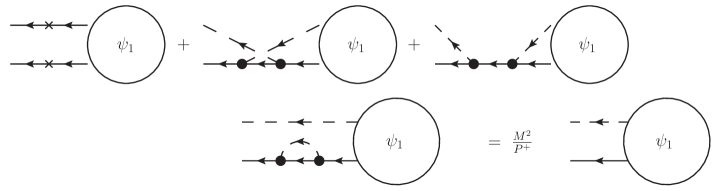
(a)

(b)

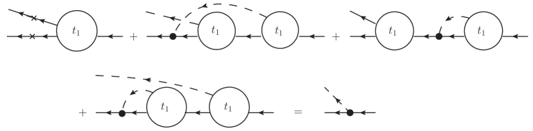
(c)

Figure 4: Graphical representations of the integral equations for (a) the Fock-state wave function $\psi_{1}$, (b) the valence state $|\phi\rangle$, and (c) the function $t_{1}$ that determines the truncated $T$ operator. The dots represent the boson emission/absorption vertex of the model Hamiltonian.

In the Fock-space truncation case, the self-energy contribution is spectator dependent, with an energy denominator that includes the second boson in flight as well as the boson in the loop. Also, the self-energy in the one-boson sector is different from the self-energy correction in bare-fermion sector. In the LFCC equations, the self-energy corrections are the same everywhere they appear and are not spectator dependent. The price paid for this gain is the nonlinear nature of the equation for $t_{1}$.

To derive the LFCC equations, we must first construct the effective Hamiltonian. This is done by computing the commutators of the Baker–Hausdorff expansion for $\overline{{\cal P}^{-}}$. The necessary commutators are represented in Fig. 5. When added to ${\cal P}^{-}$, they provide all that is needed to define the LFCC eigenvalue problem and auxiliary equations for the bare-fermion valence state with the chosen truncation of $T$. Notice that all three of the diagrams analogous to those for the Ward identity in QED are included.

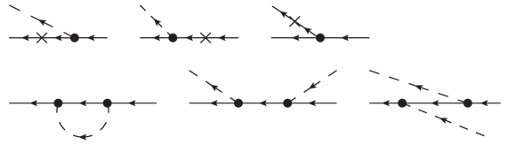
(a)

(b)

Figure 5: The commutators (a) $[{\cal P}^{-},T]$ and (b) $[[{\cal P}^{-},T],T]$ used to define the Baker–Hausdorff expansion of the LFCC effective Hamiltonian $\overline{{\cal P}^{-}}$. Only terms that connect the lowest Fock sectors, or contribute to such terms, are listed. In particular, the last two diagrams of (a) contribute to the commutator in (b).

One can show that the truncation for $T$ provides an exact solution for the model LFCC , so that this lowest-order LFCC approximation is actually exact. Solution of the left-hand eigenproblem, for $\langle\widetilde{\psi}|$, then permits calculation of the Dirac form factor from Eq. (6). Details are given in LFCC .

IV Light-front holographic QCD

The LFCC valence-sector eigenvalue problem for mesons and baryons in QCD can be approximated by models based on light-front holography holographicQCD . A factorized meson wave function in the valence ($q\bar{q}$) sector

$$\psi=e^{iL\varphi}X(x)\phi(\zeta)/\sqrt{2\pi\zeta}$$ (7)

is subject to an effective potential $\widetilde{U}$ that conserves $L_{z}$

$$\left[\frac{\mu_{1}^{2}}{x}+\frac{\mu_{2}^{2}}{1-x}-\frac{\partial^{2}}{\partial\zeta^{2}}-\frac{1-4L^{2}}{4\zeta^{2}}+\widetilde{U}\right]X(x)\phi(\zeta)=M^{2}X(x)\phi(\zeta).$$ (8)

For zero-mass quarks, the longitudinal wave function $X$ decouples, and the transverse wave function satisfies

$$\left[-\frac{d^{2}}{d\zeta^{2}}-\frac{1-4L^{2}}{4\zeta^{2}}+U(\zeta)\right]\phi(\zeta)=M^{2}\phi(\zeta),$$ (9)

with $U$ determined by an AdS₅ correspondence.

The softwall model for massless quarks softwall yields an oscillator potential $U(\zeta)=\kappa^{4}\zeta^{2}+2\kappa^{2}(J-1)$ and a simple spectrum. The masses $M^{2}=4\kappa^{2}\left(n+(J+L)/2\right)$ have a linear Regge trajectory and are a good fit for light mesons Gershtein ; Vega ; Ebert ; Branz ; Kelley . The transverse wave functions are 2D oscillator functions. The longitudinal wave function $X$ is constrained by a form-factor duality formfactormatch , between the Fock-space construction

$$F(q^{2})=\int\frac{dx\,|X(x)|^{2}}{x(1-x)}\int 2\pi\zeta d\zeta J_{0}\left(\zeta q_{\perp}\sqrt{x/(1-x)}\right)|\phi(\zeta)|^{2}$$ (10)

and the form computed in AdS₅

$$F(q^{2})=\int dx\int 2\pi\zeta d\zeta J_{0}\left(\zeta q_{\perp}\sqrt{x/(1-x)}\right)|\phi(\zeta)|^{2}.$$ (11)

Thus $X(x)=\sqrt{x(1-x)}$, when the quarks are massless.

For massive quarks, there is the ansatz by Brodsky and De Téramond ansatz , to replace $k_{\perp}^{2}/(x(1-x))$ with $k_{\perp}^{2}/x(1-x)+\mu_{1}^{2}/x+\mu_{2}^{2}/(1-x)$ in the transverse harmonic oscillator eigenfunctions, with $\mu_{i}$ as current-quark masses. This yields a longitudinal wave function of the form

$$X_{\rm BdT}(x)=N_{\rm BdT}\sqrt{x(1-x)}e^{-(\mu_{1}^{2}/x+\mu_{2}^{2}/(1-x))/2\kappa^{2}},$$ (12)

Instead of this ansatz, we use a longitudinal equation for $X$, with an effective potential from the ‘t Hooft model tHooft

$$\left[\frac{m_{1}^{2}}{x}+\frac{m_{2}^{2}}{1-x}\right]X(x)+\frac{g^{2}}{\pi}{\cal P}\int dy\frac{X(x)-X(y)}{(x-y)^{2}}-CX(x)=M_{\parallel}^{2}X(x),$$ (13)

where the $m_{i}$ are constituent masses. The ’t Hooft model, which is based on large-$N$ two-dimensional QCD, incorporates longitudinal confinement in a manner consistent with four-dimensional QCD. The solution of this equation, $X(x)$, is known tHooft ; Bergknoff to be well approximated by $x^{\beta_{1}}(1-x)^{\beta_{2}}$, with the $\beta_{i}$ subject to the constraints $m_{i}^{2}\pi/g^{2}-1+\pi\beta_{i}\cot\pi\beta_{i}=0$. For consistency, we should have $\beta_{1}=\beta_{2}=1/2$ in the zero-current-mass limit. This fixes the coupling to be $g^{2}/\pi=m_{u}^{2}=m_{d}^{2}$.

The longitudinal equation is relatively easy to solve numerically Bergknoff ; MaHiller ; MoPerry . We expand the solution as $X(x)=\sum_{n}c_{n}f_{n}(x)$ with respect to basis functions constructed from Jacobi polynomials MoPerry

$$f_{n}(x)=N_{n}x^{\beta_{1}}(1-x)^{\beta_{2}}P_{n}^{(2\beta_{2},2\beta_{1})}(2x-1).$$ (14)

The $n=0$ term represents 90% or more of the probability. The matrix representation of the longitudinal equation, for $M_{\parallel}=0$, is then

$$\left(\frac{m_{1}^{2}}{m_{u}^{2}}A_{1}+\frac{m_{2}^{2}}{m_{u}^{2}}A_{2}+B\right)\vec{c}=\xi\vec{c},$$ (15)

with $\xi\equiv C/m_{u}^{2}$ and

$$(A_{1})_{nm} = \int_{0}^{1}\frac{dx}{x}f_{n}(x)f_{m}(x),\;\;(A_{2})_{nm}=\int_{0}^{1}\frac{dx}{1-x}f_{n}(x)f_{m}(x),$$ (16)

$$B_{nm} = \frac{1}{2}\int_{0}^{1}dx\int_{0}^{1}dy\frac{f_{n}(x)-f_{n}(y)}{x-y}\frac{f_{m}(x)-f_{m}(y)}{x-y}.$$ (17)

The solution of the matrix problem yields the coefficients for the basis-function expansion.

The wave function can the be used to compute the decay constant decayconstant

$$f_{M}=2\sqrt{6}\int_{0}^{1}dx\int_{0}^{\infty}\frac{dk_{\perp}^{2}}{16\pi^{2}}\psi(x,k_{\perp})$$ (18)

and the parton distribution Vega ; pdf

$$f(x)=P_{q\bar{q}}\frac{X^{2}(x)}{x(1-x)},$$ (19)

where $P_{q\bar{q}}$ is the probability of the $q\bar{q}$ Fock component in the meson. The chosen parameter values and the resulting decay constants are listed in Table 1 for the pion, kaon, and J/$\Psi$. The wave functions and parton distributions are very similar to those of the ansatz (12), except for the J/$\Psi$, as can be seen in Figs. 6, 7, and 8.

Table 1: Parameters and decay constants, compared with the ansatz of Brodsky and De Téramond ansatz . All dimensionful parameters are in units of MeV. Parameter and experimental values are from Ref. Vega and the Particle Data Group PDG .

	model		ansatz				decay constant
meson	$m_{1}$	$m_{2}$	$\mu_{1}$	$\mu_{2}$	$P_{q\bar{q}}$	$\kappa$	model	ansatz	exper.
pion	330	330	4	4	0.204	951	131	132	130
kaon	330	500	4	101	1	524	160	162	156
J/$\Psi$	1500	1500	1270	1270	1	894	267	238	278

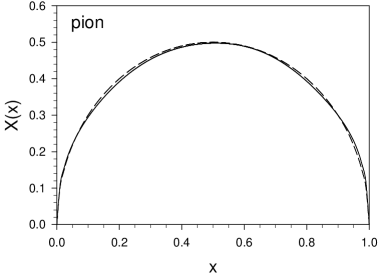
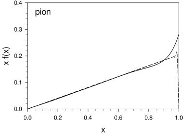
(a)	(b)

Figure 6: Longitudinal wave function (a) and parton distribution function (b) for the pion. The solid lines are wave functions from our model; the dashed lines show the ansatz by Brodsky and De Téramond ansatz .

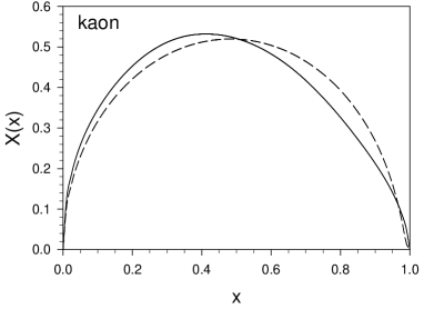
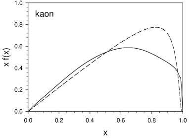
(a)	(b)

Figure 7: Same as Fig. 6, but for the kaon.

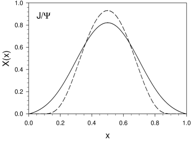
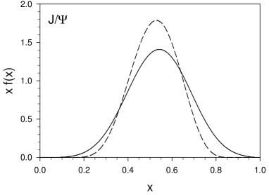
(a)	(b)

Figure 8: Same as Fig. 6, but for the J/$\Psi$.

V Summary

In order to avoid truncation of Fock space, the LFCC method LFCC generates all the higher Fock-state wave functions from the lower wave functions, based on the solution of nonlinear equations for vertex-like functions. This eliminates sector dependence and spectator dependence from the terms in the effective Hamiltonian. The truncation of the nonlinear equations can be relaxed systematically, to provide ever more sophisticated approximations for the higher wave functions.

The LFCC method divides the hadronic eigenproblem into an effective eigenproblem in the valence sector and auxiliary equations that define the effective Hamiltonian. Light-front holography holographicQCD then provides a model for the valence sector. This model can be augmented to include quark masses and a dynamical equation for the longitudinal wave function LongWF that is consistent with the Brodsky-de Téramond ansatz ansatz . The numerical solution of the longitudinal equation includes a choice of basis functions that could be useful beyond just the holographic approximation to QCD.

- (1) Chabysheva SS, Hiller, JR (2012) A light-front coupled-cluster method for the nonperturbative solution of quantum field theories. Phys. Lett. B 711: 417-422
- (2) Brodsky SJ, De Téramond GF (2006) Hadronic spectra and light-front wavefunctions in holographic QCD. Phys. Rev. Lett. 96: 201601
- (3) Chabysheva SS, Hiller JR (2013) Dynamical model for longitudinal wave functions in light-front holographic QCD. Ann. Phys. 337: 143-152
- (4) Dirac PAM (1949) Forms of relativistic dynamics. Rev. Mod. Phys. 21: 392-399
- (5) For reviews of light-cone quantization, see Burkardt M (2002) Light front quantization. Adv. Nucl. Phys. 23: 1-74; Brodsky SJ, Pauli H-C, Pinsky SS (1998) Quantum chromodynamics and other field theories on the light cone. Phys. Rep. 301: 299-486
- (6) Chabysheva SS, Hiller JR (2014) Zero modes in the light-front coupled-cluster method. Ann. Phys. 340: 188-204
- (7) Coester F (1958) Bound states of a many-particle system. Nucl. Phys. 7: 421-424; Coester F, Kümmel H (1960) Short-range correlations in nuclear wave functions. Nucl. Phys. 17: 477-485. For a recent application, see Kowalski K et al. (2004) Coupled cluster calculations of ground and excited states of nuclei. Phys. Rev. Lett. 92: 132501
- (8) Bartlett RJ, Musial M (2007) Coupled-cluster theory in quantum chemistry. Rev. Mod. Phys. 79: 291-352; Crawford TD, Schaefer HF (2000) An introduction to coupled cluster theory for computational chemists. Rev. Comp. Chem. 14: 33-136; Bishop R, Kendall AS, Wong LY, Xian Y (1993) Correlations in Abelian lattice gauge field models: A microscopic coupled cluster treatment. Phys. Rev. D 48: 887-901; Kümmel H, Lührmann KH, Zabolitzky JG (1978) Many-fermion theory in expS- (or coupled cluster) form. Phys. Rep. 36: 1-63
- (9) Čižek J (1966) On the correlation problem in atomic and molecular systems. Calculation of wavefunction components in Ursell-type expansion using quantum-field theoretical methods. J. Chem. Phys. 45: 4256-4266
- (10) Funke M, Kümmel HG (1994) Low-energy states of (1+1)-dimensional field theories via the coupled cluster method. Phys. Rev. D 50: 991-1000 and references therein; Rezaeian AH, Walet NR (2003) Renormalization of Hamiltonian field theory: A Nonperturbative and nonunitarity approach. JHEP 0312: 040; Rezaeian AH, Walet NR (2003) Linked cluster Tamm–Dancoff field theory. Phys. Lett. B 570: 129-136
- (11) Brodsky SJ, Drell SD (1980) The anomalous magnetic moment and limits on fermion substructure. Phys. Rev. D 22: 2236-2243
- (12) Brodsky SJ, Hiller JR, McCartor G (1998) Pauli-Villars regulator as a nonperturbative ultraviolet regularization scheme in discretized light-cone quantization. Phys. Rev. D 58: 025005
- (13) Greenberg OW, Schweber SS (1958) Clothed particle operators in simple models of quantum field theory. N Cim. 8: 378-406
- (14) Karch A, Katz E, Son DT, Stephanov MA (2006) Linear confinement and AdS/QCD. Phys. Rev. D 74: 015005
- (15) Gershtein SS, Likhoded AK, Luchinsky AV (2006) Systematics of heavy quarkonia from Regge trajectories on (,) and (,) planes. Phys. Rev. D 74: 016002
- (16) Vega A, Schmidt I, Branz T, Gutsche T, Lyubovitskij VE (2009) Meson wave function from holographic models. Phys. Rev. 80: 055014
- (17) Ebert D, Faustov RN, Galkin VO (2010) Heavy-light meson spectroscopy and Regge trajectories in the relativistic quark model. Eur. Phys. J. C 66: 197-206
- (18) Branz T, Gutsche T, Lyubovitskij VE, Schmidt I, Vega A (2010) Light and heavy mesons in a soft-wall holographic approach. Phys. Rev. D 82: 074022; Gutsche T, Lyubovitskij VE, Schmidt I, Vega A (2012) Dilaton in a soft-wall holographic approach to mesons and baryons. Phys. Rev. D 85: 076003
- (19) Kelley TM, Bartz SP, Kapusta J, (2011) Pseudoscalar Mass Spectrum in a Soft-Wall Model of AdS/QCD. Phys. Rev. D 83: 016002
- (20) Brodsky SJ, de Téramond GF (2008) Light-front dynamics and AdS/QCD correspondence: The pion form factor in the space and time-like regions. Phys. Rev. D 77: 056007
- (21) Brodsky SJ, de Téramond GF (2008) AdS/CFT and Light-Front QCD. arXiv:0802.0514
- (22) ’t Hooft G (1974) A two-dimensional model for mesons. Nucl. Phys. B 75: 461-470
- (23) Bergknoff H (1977) Physical particles of the massive Schwinger model. Nucl. Phys. B 122: 215-236
- (24) Ma Y, Hiller JR (1989) Numerical solution of the one-pair equation in the massive Schwinger model. J. Comput. Phys. 82: 229-240
- (25) Mo Y, Perry RJ (1993) Basis function calculations for the massive Schwinger model in the light front Tamm-Dancoff approximation. J. Comput. Phys. 108: 159-174
- (26) Brodsky SJ, Huang T, Lepage GP (1983) Hadronic wave functions and high momentum transfer interactions in quantum chromodynamics. In: Capri AZ, Kamal AN (ed.) Proceedings of the Banff Summer Institute on Particles and Fields 2, Banff, Alberta, 1981, 143-199. Plenum, New York; Lepage GP, Brodsky SJ, Huang T, Mackenzie PB (1983) Hadronic wave functions in QCD. ibid., 83-142; Huang T (1980) Hadron wave functions and structure functions in QCD. AIP Conf. Proc. 68: 1000-1004
- (27) Radyushkin AV (1998) Nonforward parton densities and soft mechanism for form-factors and wide angle Compton scattering in QCD. Phys. Rev. D 58: 114008
- (28) Nakamura K et al. (Particle Data Group) (2010) Review of particle physics. J. Phys. G 37: 075021