Thresholds of absorbing sets in
Low-Density-Parity-Check codes

Abstract

In this paper, we investigate absorbing sets, responsible of error floors in Low Density Parity Check codes. We look for a concise, quantitative way to rate the absorbing sets’ dangerousness. Based on a simplified model for iterative decoding evolution, we show that absorbing sets exhibit a threshold behavior. An absorbing set with at least one channel log-likelihood-ratio below the threshold can stop the convergence towards the right codeword. Otherwise convergence is guaranteed. We show that absorbing sets with negative thresholds can be deactivated simply using proper saturation levels. We propose an efficient algorithm to compute thresholds.

I Introduction

In the last years much effort has been spent to identify the weak points of Low Density Parity Check (LDPC) code graphs, responsible for error floors of iterative decoders. After the introduction of the seminal concept of pseudocodewords [1],[2] it is now ascertained that these errors are caused by small subsets of nodes of the Tanner graph that act as attractors for iterative decoders, even if they are not the support of valid codewords. These structures have been named trapping sets [3],[4],[5] or absorbing sets [6],[7],[8] or absorption sets [9], defined in slightly different ways. In this paper we build mainly on [9] and [6],[8],[10].

The first merit of [6],[10] has been to define Absorbing Sets (ASs) from a purely topological point of view. Moreover, the authors have analyzed the effects of ASs on finite precision iterative decoders, on the basis of hardware and Importance Sampling simulations [8],[7]. ASs behavior depends on the decoder quantization and in [8] they are classified as weak or strong depending on whether they can be resolved or not by properly tuning the decoder dynamics. In [11] the same research group proposes a postprocessing method to resolve ASs, once the iterative decoder is trapped.

In [9] the author defines absorption sets (equivalent to ASs) and identifies a variety of ASs for the LDPC code used in the IEEE 802.3an standard. The linear model of [12], suitable for Min-Sum (MS) decoding, is refined to meet the behavior of belief propagation decoders. Under some hypotheses, the error probability level can be computed assuming an unsaturated LDPC decoder. Loosely speaking, in this model an AS is solved if messages coming from the rest of the graph tend to infinity with a rate higher than the wrong messages inside the AS. In practical implementations, messages cannot get arbitrarily large. Besides, hypotheses on the growth rate of the messages entering the AS are needed. In [9] Density Evolution (DE) is used, but this is accurate only for LDPC codes with infinite (in practice, very large) block lengths. In [13] the saturation is taken into account and the input growth rate is evaluated via Discretized DE or empirically via simulation.

In [4] and successive works, the authors rate the trapping set dangerousness with the critical number, that is valid for hard decoders but fails to discriminate between the soft entries of the iterative decoder.

In this paper, we look for a concise, quantitative way to rate the ASs’ dangerousness with soft decoding. We focus on Min-Sum (MS) soft decoding that is the basis for any LDPC decoder implementation, leaving aside more theoretical algorithms such as Sum-Product (SPA) or Linear Programming (LP). We study the evolution of the messages propagating inside the AS, when the all-zero codeword is transmitted. Unlike [9], we assume a limited dynamic of the Log Likelihood Ratios (LLRs) as in a practical decoder implementation. The AS dangerousness can be characterized by a threshold $\tau$. We show that, under certain hypotheses, the decoder convergence towards the right codeword can fail only if there exist channel LLRs smaller than or equal to $\tau$. When all channel LLRs are larger than $\tau$, successful decoding is assured. We also show with examples that ASs with greater $\tau$ are more harmful than ASs with smaller $\tau$. Finally, we provide an efficient algorithm to find $\tau$.

For many ASs, $\tau<0$. In these cases we can deactivate ASs simply setting two saturation levels, one for extrinsic messages (in our system model, this level is normalized to $1$), and another level, smaller than $|\tau|$, for channel LLRs. This way the code designer can concentrate all efforts on avoiding only the most dangerous ASs, letting the receiver automatically deactivate the other ones with extrinsic messages strong enough to unlock them.

The article is organized as follows. Section II settles the system model. Section III introduces the notion of equilibria and thresholds. Section IV deals with generalized equilibria, a tool to study ASs with arbitrary structure. Section V deals with limit cycles. Section VI studies the message passing behavior above threshold, and provides a method to deactivate many ASs. Section VII shows practical examples of ASs that behave as predicted by our model during MS decoding on real complete LDPC graphs. Section VIII proposes an efficient algorithm to compute $\tau$. Section IX highlights other interesting properties. Finally, Section X concludes the paper.

II System model and definitions

We recall that a subset $\mathcal{D}$ of variable nodes (VNs) in a Tanner graph is an absorbing set $(a,b)$ if [6]

• every VN in $\mathcal{D}$ has strictly more boundary Check Nodes (CNs) in $\mathcal{E}(\mathcal{D})$ than in $\mathcal{O}(\mathcal{D})$, being $\mathcal{E}(\mathcal{D})$ and $\mathcal{O}(\mathcal{D})$ the set of boundary CNs connected to $\mathcal{D}$ an even or odd number of times, respectively;

• the cardinality of $\mathcal{D}$ and $\mathcal{O}(\mathcal{D})$ are $a$ and $b$, respectively.

Besides, $\mathcal{D}$ is a fully absorbing set if also all VNs outside $\mathcal{D}$ have strictly less neighbors in $\mathcal{O}(\mathcal{D})$ than outside. In [10] it is observed that a pattern of all-ones for the VNs in $\mathcal{D}$ is a stable concurrent of the all-zeros pattern for the iterative bit-flipping decoder, notwithstanding a set $\mathcal{O}(\mathcal{D})$ of unsatisfied boundary CNs (dark CNs in Fig. 1). ASs behave in a similar manner also under iterative soft decoding, as shown and discussed in [8], [7].

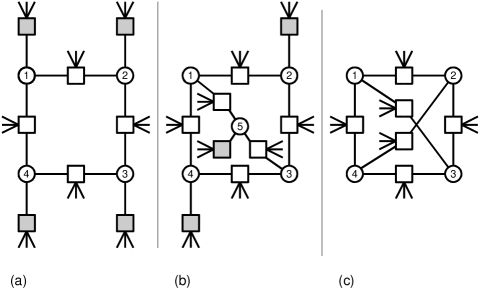
Figure 1: Three absorbing sets: in Fig. 1(a), a maximal $(4,4)$ AS; in Fig. 1(b), a $(5,3)$ AS; in Fig. 1(c), a $(4,0)$ AS, that is also the support of a codeword.

If all CNs are connected to $\mathcal{D}$ no more than twice, the AS is elementary. Elementary ASs are usually the most dangerous. Given the code girth, elementary absorbing sets can have smaller values of $a$ and $b$ than non elementary ones [14]. If ASs are the support of near-codewords [15], the smaller $a$ is, the higher the probability of error. Besides, the smaller the ratio $b/a$, the more dangerous the AS is [8]. In this paper we focus on elementary ASs only, as those in Fig. 1. An AS is maximal if $a=b$, as in Fig. 1(a). Intuitively, maximal ASs are the mildest ones, since they have a large number of unsatisfied CNs. On the opposite, an AS with $b=0$ (as in Fig. 1(c)) is the support of a codeword.

For our analysis we assume an MS decoder, that is insensitive to scale factors. Thus we can normalize the maximum extrinsic message amplitude. We recall that, apart from saturation, the evolution of the messages inside the AS is linear ([9], [12]) since the CNs in $\mathcal{E}(\mathcal{D})$ simply forward the input messages. The relation among the $N=2|\mathcal{E}(\mathcal{D})|$ internal extrinsic messages $\mathbf{x}$ generated by VNs can be tracked during the iterations, by an $N\times N$ routing matrix $\mathbf{A}$. Basically, $A_{i,j}=1$ iff there exists an (oriented) path from message $x_{j}$ to message $x_{i}$, going across one VN. For instance, Fig. 2 depicts the LLR exchange within the AS of Fig. 1(b). The corresponding first row of $\mathbf{A}$ is

$$\mathbf{A}_{\{1\},\{1,\ldots,N\}}=\left[\;0\;\;0\;\;0\;\;0\;\;0\;\;0\;\;0\;\;0\;\;0\;\;1\;\;1\;\;0\;\right]\,.$$ (1)

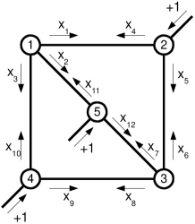
Figure 2: Message propagation within the AS of Fig. 1(b). For simplicity, CNs in the middle of edges are not shown.

To account for saturation we define the scalar function $\mathrm{sat}(x)\triangleq\mathrm{sign}(x)\cdot\min\left(|x|,1\right)$ and we say that $x$ is saturated if $|x|\geq 1$, unsaturated otherwise. For vectors, $\mathrm{sat}(\mathbf{x})$ is the element-wise saturation.

For the time being, we consider a parallel message passing decoder, where all VNs are simultaneously activated first, then all CNs are simultaneously activated, in turn. The system evolution at the $k$-th iteration reads

$$\mathbf{x}^{(k+1)}=\mathrm{sat}\left(\mathbf{A}\mathbf{x}^{(k)}+\mathbf{e}+\mathbf{R}\boldsymbol{\lambda}\right)$$ (2)

where $\mathbf{x}^{(k)}$ are the extrinsic messages within the AS, $\mathbf{e}$ is the vector of extrinsic messages entering the AS through $\mathcal{O}(\mathcal{D})$, and $\mathbf{R}$ is a repetition matrix with size $N\times a$, that constrains the $a$ channel LLRs $\boldsymbol{\lambda}$ to be the same for all messages $x_{j}$ emanating from the same VN. Referring to Fig. 1(b),

$$\mathbf{R}^{T}=\setcounter{MaxMatrixCols}{12}\begin{bmatrix}1&1&1&0&0&0&0&0&0&0&0&0\\ 0&0&0&1&1&0&0&0&0&0&0&0\\ 0&0&0&0&0&1&1&1&0&0&0&0\\ 0&0&0&0&0&0&0&0&1&1&0&0\\ 0&0&0&0&0&0&0&0&0&0&1&1\\ \end{bmatrix}\,.$$ (3)

Also note that the row weight of $\mathbf{R}$ is unitary, i.e. $\mathbf{R}\mathbf{1}=\mathbf{1}$.

As to the extrinsic messages entering the AS from outside, we bypass the tricky problem of modeling the dynamical behavior of the decoder in the whole graph assuming that each message entering the AS has saturated to the maximal correct LLR (i.e. $+1$, since we transmit the all-zero codeword). This is a reasonable hypothesis after a sufficient number of iterations, as observed in [11] where the authors base their postprocessing technique on this assumption. In Section VII we show that the decoding of a large graph is in good agreement with the predictions of this model. Under this hypothesis, we can write

$$\mathbf{e}=\mathbf{R}\mathbf{d}-\mathbf{1}-\mathbf{A}\mathbf{1}$$ (4)

where $\mathbf{d}$ is the $a\times 1$ vector of the VN degrees.

From now on, we will consider only left-regular LDPC codes, with $d_{i}=3,\;\forall i$. Most of the theorems presented in the following sections can be extended to a generic VN degree vector $\mathbf{d}$. Luckily, among regular LDPC codes this is also the case with the most favorable waterfall region. If we set $\mathbf{d}=3\cdot\mathbf{1}$, then $\mathbf{Rd}-\mathbf{1}=3\cdot\mathbf{R1}-\mathbf{1}=3\cdot\mathbf{1}-\mathbf{1}=2\cdot\mathbf{1}$, and (2) becomes

$$\mathbf{x}^{(k+1)}=\mathrm{sat}\left(\mathbf{A}\left(\mathbf{x}^{(k)}-\mathbf{1}\right)+2\cdot\mathbf{1}+\mathbf{R}\boldsymbol{\lambda}\right)\,.$$ (5)

This equation is more expressive than (2), as $\mathbf{x}^{(k)}-\mathbf{1}$ is the gap between the current state $\mathbf{x}^{(k)}$ and the values that the extrinsic messages should eventually achieve, once the AS is unlocked. Besides, we will show that $-\mathbf{1}\leq\boldsymbol{\lambda}\leq\mathbf{1}$. Therefore, $2\cdot\mathbf{1}+\mathbf{R}\boldsymbol{\lambda}\geq\mathbf{1}$ and $\mathbf{A}\left(\mathbf{x}^{(k)}-\mathbf{1}\right)\leq\mathbf{0}$. The two competing forces are now clearly visible. The former always helps convergence, and the latter can amplify negative terms (if the AS is not maximal, some rows of $\mathbf{A}$ have weight larger than $1$).

The rest of the paper is devoted to unveil the hidden properties of (5), finding sufficient conditions for correct decoding, i.e. $\mathbf{x}^{(k)}\rightarrow\mathbf{1}$ when $k\rightarrow\infty$. We will assume a conservative condition to decouple the AS behavior from the rest of the code: we do not start with $\mathbf{x}^{(0)}=\mathbf{0}$. We take into account any configuration of extrinsic messages $\mathbf{x}^{(0)}$ that may result in a convergence failure. We start from an iteration with the rest of the decoder messages saturated to $1$. The configuration $\mathbf{x}^{(0)}$ inside the AS, which is the result of the message evolution up to that iteration, is unknown. The drawback of this approach is that we renounce to predict the probability of message configurations inside the AS leading to decoding errors. On the other hand, if no $\mathbf{x}^{(0)}$ can lock the decoder, this is true independently of the evolution of messages inside the AS. We will study equilibria, limit cycles and chaotic behaviors (i.e., aperiodic trajectories) of (5), depending on the channel LLRs $\boldsymbol{\lambda}$ and any initial state $\mathbf{x}^{(0)}$.

III Equilibria, threshold definition and preliminary properties

In this Section, we study equilibria for the non-linear system (5).

Definition III.1.

A pair $(\mathbf{x},\boldsymbol{\lambda})$ is an equilibrium iff

$$\mathbf{x}=\mathrm{sat}\left(\mathbf{A}\left(\mathbf{x}-\mathbf{1}\right)+2\cdot\mathbf{1}+\mathbf{R}\boldsymbol{\lambda}\right)\,.$$ (6)

Equilibria with $\mathbf{x}\neq\mathbf{1}$ are harmful. They behave as attractors for the evolution of the extrinsic messages $\mathbf{x}^{(k)}$, and can lead to uncorrect decisions. With the aim of finding the most critical ASs, those that can lead to convergence failure even with large values of $\boldsymbol{\lambda}$, we would like to solve the following problem:

Problem III.1.

$$\tau^{\prime}=\max_{\boldsymbol{\lambda},\mathbf{x}} \quad\min(\boldsymbol{\lambda})$$

$$s.t. \quad-\mathbf{1}\leq\mathbf{x}\leq\mathbf{1},\quad\exists j:x_{j}<1$$ (7)

$$\quad\mathbf{x}=\mathrm{sat}\left(\mathbf{A}\left(\mathbf{x}-\mathbf{1}\right)+2\cdot\mathbf{1}+\mathbf{R}\boldsymbol{\lambda}\right)\,.$$

The constraint (7) restricts the search to bad equilibria, having at least one extrinsic message smaller than $1$. We call $\tau^{\prime}$ the threshold, since the AS has no bad equilibria with $\boldsymbol{\lambda}$ above that value. In Section VI we will show that the notion of threshold does not pertain only to bad equilibria, but also to any other bad trajectory of (5), not achieving $\mathbf{x}^{(\infty)}=\mathbf{1}$.

In the above optimization problem, for simplicity we did not assign upper and lower bounds to the channel LLRs $\boldsymbol{\lambda}$. In practice, we can restrict our search in the range $-\mathbf{1}\leq\boldsymbol{\lambda}\leq\mathbf{1}$.

Theorem III.1.

The pair $(\mathbf{x}=-\mathbf{1},\boldsymbol{\lambda}=-\mathbf{1})$ is always an equilibrium.

Proof:

Substituting $(\mathbf{x}=-\mathbf{1},\boldsymbol{\lambda}=-\mathbf{1})$ in the equilibrium equation, we obtain

$$\mathrm{sat}\left(\mathbf{A}\left(\mathbf{x}-\mathbf{1}\right)+2\cdot\mathbf{1}+\mathbf{R}\boldsymbol{\lambda}^{\prime}\right)=\mathrm{sat}\left(-2\cdot\underbrace{\mathbf{A}\mathbf{1}}_{\geq\mathbf{1}}+\mathbf{1}\right)\\ =-\mathbf{1}=\mathbf{x}\,.$$ (8)

∎

Theorem III.2.

The only equilibrium $(\mathbf{x},\boldsymbol{\lambda})$ for a system having $\boldsymbol{\lambda}>\mathbf{1}$ and $-\mathbf{1}\leq\mathbf{x}\leq\mathbf{1}$ is in $\mathbf{x}=\mathbf{1}$.

Proof:

Since $\boldsymbol{\lambda}>\mathbf{1}$, we can define a strictly positive quantity $\Delta\triangleq\min(\boldsymbol{\lambda})-1>0$. Consider parallel message passing. Focusing on the evolution of (5),

$$\mathbf{x}^{(1)}=\mathrm{sat}\left(\mathbf{A}\underbrace{(\mathbf{x}^{(0)}-\mathbf{1})}_{\geq-2\cdot\mathbf{1}}+\underbrace{2\cdot\mathbf{1}+\mathbf{R}\boldsymbol{\lambda}}_{\geq(3+\Delta)\mathbf{1}}\right)\\ \geq\mathrm{sat}\left(-2\underbrace{\mathbf{A}\mathbf{1}}_{\leq 2\cdot\mathbf{1}}+(3+\Delta)\mathbf{1}\right)\geq\mathrm{sat}(-1+\Delta)\cdot\mathbf{1}\,.$$ (9)

If $\mathrm{sat}(-1+\Delta)=1$, then $\mathbf{x}^{(1)}=\mathbf{1}$, and we stop. Otherwise, $\mathrm{sat}(-1+\Delta)=-1+\Delta$ and we go on. For the generic step, assuming $\mathbf{x}^{(k)}\geq\mathrm{sat}\left(-1+k\Delta\right)\cdot\mathbf{1}$ and proceeding by recursion, we have

$$\mathbf{x}^{(k+1)}=\mathrm{sat}\left(\mathbf{A}\underbrace{(\mathbf{x}^{(k)}-\mathbf{1})}_{\geq(-2+k\Delta)\cdot\mathbf{1}}+\underbrace{2\cdot\mathbf{1}+\mathbf{R}\boldsymbol{\lambda}}_{\geq(3+\Delta)\mathbf{1}}\right)\\ \geq\mathrm{sat}\left(-\mathbf{1}+k\Delta\underbrace{\mathbf{A}\mathbf{1}}_{\geq\mathbf{1}}+\Delta\mathbf{1}\right)\geq\mathrm{sat}\left(-1+(k+1)\Delta\right)\cdot\mathbf{1}\,.$$ (10)

The same inequalities hold also in case of sequential message passing, activating CNs in arbitrary order (once per iteration).

As soon as $-1+(k+1)\Delta\geq 1$, the recursion ends. We conclude that the message passing algorithm will eventually achieve $\mathbf{x}=\mathbf{1}$. ∎

Being $\tau^{\prime}$ the result of a maximization, a straight consequence of the above two theorems is

Corollary III.1.

As for Problem III.1, $-1\leq\tau^{\prime}\leq 1$.

The two boundary values $\tau^{\prime}=-1$ and $\tau^{\prime}=1$ are the thresholds of maximal ASs and codewords, respectively:

Theorem III.3.

Any support of a codeword has $\tau^{\prime}=1$. Maximal absorbing sets have $\tau^{\prime}=-1$.

Proof:

We start from codewords. $(\mathbf{x}=-\mathbf{1},\boldsymbol{\lambda}=\mathbf{1})$ is a valid equilibrium for Problem III.1. Indeed:

$$\mathrm{sat}\left(\mathbf{A}(\mathbf{x}-\mathbf{1})+2\cdot\mathbf{1}+\mathbf{R}\boldsymbol{\lambda}\right)=\mathrm{sat}\left(-2\underbrace{\mathbf{A}\mathbf{1}}_{=2\cdot\mathbf{1}}+3\cdot\mathbf{1}\right)\\ =\mathrm{sat}\left(-4\cdot\mathbf{1}+3\cdot\mathbf{1}\right)=-\mathbf{1}=\mathbf{x}\,.$$ (11)

By Corollary III.1 we conclude that $\tau^{\prime}=1$.

Referring to maximal ASs, for any $-\mathbf{1}\leq\mathbf{x}^{(0)}\leq\mathbf{1}$ and $\boldsymbol{\lambda}>-\mathbf{1}$, we can define a strictly positive quantity $\Delta\triangleq\min(\boldsymbol{\lambda})-(-1)>0$. Focusing on the evolution of (5),

$$\mathbf{x}^{(1)}=\mathrm{sat}\left(\mathbf{A}\underbrace{(\mathbf{x}^{(0)}-\mathbf{1})}_{\geq-2\cdot\mathbf{1}}+\underbrace{2\cdot\mathbf{1}+\mathbf{R}\boldsymbol{\lambda}}_{\geq(1+\Delta)\mathbf{1}}\right)\\ \geq\mathrm{sat}\left(-2\underbrace{\mathbf{A}\mathbf{1}}_{=\mathbf{1}}+(1+\Delta)\mathbf{1}\right)\geq\mathrm{sat}(-1+\Delta)\cdot\mathbf{1}\,.$$ (12)

If $\mathrm{sat}(-1+\Delta)=1$, then $\mathbf{x}^{(1)}=\mathbf{1}$, and we stop. Otherwise, $\mathrm{sat}(-1+\Delta)=-1+\Delta$ and we go on. For the generic step, assuming $\mathbf{x}^{(k)}\geq\mathrm{sat}\left(-1+k\Delta\right)\cdot\mathbf{1}$ and proceeding by recursion, we obtain

$$\mathbf{x}^{(k+1)}=\mathrm{sat}\left(\mathbf{A}\underbrace{(\mathbf{x}^{(k)}-\mathbf{1})}_{\geq(-2+k\Delta)\cdot\mathbf{1}}+\underbrace{2\cdot\mathbf{1}+\mathbf{R}\boldsymbol{\lambda}}_{\geq(1+\Delta)\mathbf{1}}\right)\\ \geq\mathrm{sat}\left(-1+(k+1)\Delta\right)\cdot\mathbf{1}\,.$$ (13)

As soon as $-1+(k+1)\Delta\geq 1$, the recursion ends. The message passing algorithm will eventually achieve $\mathbf{x}=\mathbf{1}$, that is not a valid equilibrium for Problem III.1. We conclude that at least one element in $\boldsymbol{\lambda}$ must be equal to $-1$, therefore $\tau^{\prime}=-1$. ∎

IV Generalized equilibria

Most of the effort of this Section is in the reformulation of Problem III.1, to make it manageable. First, in place of equilibria, we consider a slightly more general case, removing the repetition matrix $\mathbf{R}$ and assuming $N$ unconstrained channel LLRs $\boldsymbol{\lambda}$.

Definition IV.1.

A pair $(\mathbf{x},\boldsymbol{\lambda})$ is a generalized equilibrium iff

$$\mathbf{x}=\mathrm{sat}\left(\mathbf{A}\left(\mathbf{x}-\mathbf{1}\right)+2\cdot\mathbf{1}+\boldsymbol{\lambda}\right)\,.$$ (14)

Accordingly, we write the following optimization problem.

Problem IV.1.

$$\tau^{*}=\max_{\boldsymbol{\lambda},\mathbf{x}} \quad\min(\boldsymbol{\lambda})$$

$$s.t. \quad-\mathbf{1}\leq\mathbf{x}\leq\mathbf{1},\quad\exists j:x_{j}<1$$

$$\quad\mathbf{x}=\mathrm{sat}\left(\mathbf{A}\left(\mathbf{x}-\mathbf{1}\right)+2\cdot\mathbf{1}+\boldsymbol{\lambda}\right).$$

The following theorem holds.

Theorem IV.1.

As for Problems III.1 and IV.1, $\tau^{\prime}=\tau^{*}$.

Proof:

We show that $\tau^{\prime}\leq\tau^{*}$ and $\tau^{\prime}\geq\tau^{*}$.

Every equilibrium is also a generalized equilibrium. Given a solution $(\mathbf{x}^{\prime},\boldsymbol{\lambda}^{\prime})$ of Problem III.1 with $\min(\boldsymbol{\lambda}^{\prime})=\tau^{\prime}$, the solution $(\mathbf{x}^{*},\boldsymbol{\lambda}^{*})$ with $\mathbf{x}^{*}=\mathbf{x}^{\prime}$ and $\boldsymbol{\lambda}^{*}=\mathbf{R}\boldsymbol{\lambda}^{\prime}$ satisfies the constraints of Problem III.1. Being $\tau^{*}$ the result of the maximization in Problem IV.1, we conclude that $\tau^{*}\geq\tau^{\prime}$.

On the converse, generalized equilibria may not be equilibria. Indeed, $\boldsymbol{\lambda}^{*}$ could not be compatible with the repetition forced by matrix $\mathbf{R}$. Notwithstanding this, if a generalized equilibrium $(\mathbf{x}^{*},\boldsymbol{\lambda}^{*})$ exists, then also an equilibrium $(\mathbf{x}^{\prime},\boldsymbol{\lambda}^{\prime})$ exists, with $\mathbf{x}^{\prime}\leq\mathbf{x}^{*}$ and $\boldsymbol{\lambda}^{\prime}=\min(\boldsymbol{\lambda}^{*})\cdot\mathbf{1}$. Consider channel LLRs $\boldsymbol{\lambda}^{\prime}=\min(\boldsymbol{\lambda}^{*})\cdot\mathbf{1}$. We explicitly provide an initialization $\mathbf{x}^{(0)}$ for (5) that makes the extrinsic messages achieve an equilibrium $(\mathbf{x}^{\prime},\boldsymbol{\lambda}^{\prime})$, with $\mathbf{x}^{\prime}\leq\mathbf{x}^{*}$. First, note that

$$\mathbf{x}^{(k+1)}=\mathrm{sat}\left(\mathbf{A}\left(\mathbf{x}^{(k)}-\mathbf{1}\right)+2\cdot\mathbf{1}+\mathbf{R}\boldsymbol{\lambda}^{\prime}\right)\\ =\mathrm{sat}\left(\mathbf{A}\left(\mathbf{x}^{(k)}-\mathbf{1}\right)+2\cdot\mathbf{1}+\min(\boldsymbol{\lambda}^{*})\underbrace{\mathbf{R}\mathbf{1}}_{=\mathbf{1}}\right)\,.$$ (15)

If we set $\mathbf{x}^{(0)}=\mathbf{x}^{*}$, we obtain the inequality

$$\mathbf{x}^{(1)}=\mathrm{sat}\left(\mathbf{A}\left(\mathbf{x}^{*}-\mathbf{1}\right)+2\cdot\mathbf{1}+\min(\boldsymbol{\lambda}^{*})\mathbf{1}\right)\\ \leq\mathrm{sat}\left(\mathbf{A}\left(\mathbf{x}^{*}-\mathbf{1}\right)+2\cdot\mathbf{1}+\boldsymbol{\lambda}^{*}\right)=\mathbf{x}^{*}=\mathbf{x}^{(0)}\,.$$ (16)

Proceeding by induction,

$$\mathbf{x}^{(k+1)}=\mathrm{sat}\left(\mathbf{A}\left(\mathbf{x}^{(k)}-\mathbf{1}\right)+2\cdot\mathbf{1}+\min(\boldsymbol{\lambda}^{*})\mathbf{1}\right)\\ \leq\mathrm{sat}\left(\mathbf{A}\left(\mathbf{x}^{(k-1)}-\mathbf{1}\right)+2\cdot\mathbf{1}+\min(\boldsymbol{\lambda}^{*})\mathbf{1}\right)=\mathbf{x}^{(k)}$$ (17)

since $A_{i,j}\geq 0,\;\forall i,j$. The above equation states that the sequence $\{\mathbf{x}^{(k)}\}$ is monotonically decreasing. Yet, it cannot assume arbitrarily small values, since extrinsic messages have a lower saturation to $-1$. We conclude that $\{\mathbf{x}^{(k)}\}$ must achieve a new equilibrium $\mathbf{x}^{\prime}\leq\mathbf{x}^{*}$.

The equilibrium $(\mathbf{x}^{\prime},\boldsymbol{\lambda}^{\prime})$ satisfies all the constraints of Problem III.1. Being $\tau^{\prime}$ the result of a maximization, $\tau^{\prime}\geq\tau^{*}$. ∎

The above statements do not claim that the two problems are equivalent. Indeed, they can be maximized by different pairs $(\mathbf{x},\boldsymbol{\lambda})$. Anyway, as long as we are interested in the AS threshold, we can deal with Problem IV.1 instead of Problem III.1 and with generalized equilibria instead of equilibria.

V Limit cycles

In this Section, we focus on limit cycles, i.e. on extrinsic messages that periodically take the same values. We show that they have thresholds smaller than or equal to equilibria. Therefore, we will neglect them.

Definition V.1.

The sequence $(\{\mathbf{x}^{\prime\prime(0)},\ldots,\mathbf{x}^{\prime\prime(L-1)}\},\boldsymbol{\lambda}^{\prime\prime})$ is a limit cycle with period $L$ iff $\forall k$,

$$\mathbf{x}^{\prime\prime(k+1\>\mathrm{mod}\>L)}=\mathrm{sat}\left(\mathbf{A}\left(\mathbf{x}^{\prime\prime(k\>\mathrm{mod}\>L)}-\mathbf{1}\right)+2\cdot\mathbf{1}+\mathbf{R}\boldsymbol{\lambda}^{\prime\prime}\right)\,.$$ (18)

Limit cycles can be interpreted as equilibria of the augmented AS, described by an augmented matrix $\mathbf{A}^{\prime\prime}$ of size $(NL)\times(NL)$. While the VN and CN activation order does not matter in case of equilibria (at the equilibrium, extrinsic messages do not change if we update them all together, or one by one in arbitrary order), this is not true in case of limit cycles. Indeed, the associated set of equations depends on the decoding order.

In case of parallel message passing, one can write a system of equations with $NL$ rows, where the $l$-th horizontal stripe of $N$ equations represents the evolution of extrinsic messages from state $\mathbf{x}^{\prime\prime(l-1\mod L)}$ to $\mathbf{x}^{\prime\prime(l)}$

$$\begin{bmatrix}\mathbf{x}^{\prime\prime(0)}\\ \mathbf{x}^{\prime\prime(1)}\\ \vdots\\ \mathbf{x}^{\prime\prime(L-1)}\\ \end{bmatrix}=\mathrm{sat}\left(\mathbf{A}^{\prime\prime}\left(\begin{bmatrix}\mathbf{x}^{\prime\prime(0)}\\ \mathbf{x}^{\prime\prime(1)}\\ \vdots\\ \mathbf{x}^{\prime\prime(L-1)}\\ \end{bmatrix}-\mathbf{1}\right)+2\cdot\mathbf{1}+\begin{bmatrix}\mathbf{R}\boldsymbol{\lambda}^{\prime\prime}\\ \mathbf{R}\boldsymbol{\lambda}^{\prime\prime}\\ \vdots\\ \mathbf{R}\boldsymbol{\lambda}^{\prime\prime}\\ \end{bmatrix}\right)\,.$$ (19)

Instead, in sequential (or serial-C [16]) decoding CNs are activated one by one, in turn, immediately updating the a-posteriori LLRs of the VNs connected thereto. The augmented matrix changes, since only the first CNs use extrinsic messages produced at the previous iteration, while all others exploit messages generated during the same iteration. We can represent this behavior defining two matrices $\mathbf{\bar{A}}$ and $\mathbf{\underline{A}}$, binary partitions of $\mathbf{A}$,

$$\bar{A}_{i,j},\underline{A}_{i,j}\in\{0,1\},\qquad\mathbf{\bar{A}}+\mathbf{\underline{A}}=\mathbf{A}$$ (20)

and writing an augmented matrix as

$$\mathbf{A}^{\prime\prime}=\begin{bmatrix}\mathbf{\underline{A}}&\mathbf{0}&\cdots&\mathbf{0}&\mathbf{\bar{A}}\\ \mathbf{\bar{A}}&\mathbf{\underline{A}}&\cdots&\mathbf{0}&\mathbf{0}\\ \mathbf{0}&\mathbf{\bar{A}}&&\mathbf{0}&\mathbf{0}\\ \vdots&\vdots&\ddots&\ddots&\vdots\\ \mathbf{0}&\mathbf{0}&\cdots&\mathbf{\bar{A}}&\mathbf{\underline{A}}\\ \end{bmatrix}\,.$$ (21)

$\bar{\mathbf{A}}$ and $\underline{\mathbf{A}}$ have upper and lower triangular shapes, due to the sequential update order. Note that (21) is valid not only for sequential CN message passing decoding, but also for any arbitrary order, as long as all extrinsic messages are activated in turn, once per decoding iteration. Parallel message passing is a special case of (21), with $\mathbf{\bar{A}}=\mathbf{A}$ and $\mathbf{\underline{A}}=\mathbf{0}$. Therefore we provide the following theorem only for the most general case.

Theorem V.1.

If there exists a limit cycle $(\{\mathbf{x}^{\prime\prime(0)},\mathbf{x}^{\prime\prime(1)},\ldots,\mathbf{x}^{\prime\prime(L-1)}\},\boldsymbol{\lambda}^{\prime\prime})$, a generalized equilibrium $(\mathbf{x}^{*},\boldsymbol{\lambda}^{*})$ with $\boldsymbol{\lambda}^{*}\geq\mathbf{R}\boldsymbol{\lambda}^{\prime\prime}$ exists, too.

Proof:

Consider any partition of the identity matrix $\mathbf{I}$ in $L$ binary matrices, with size $N\times N$:

$$W_{i,j}^{(l)}\in\{0,1\},\qquad\sum_{l=0}^{L-1}\mathbf{W}^{(l)}=\mathbf{I}\,.$$ (22)

Then

$$\sum_{l=0}^{L-1}\mathbf{W}^{(l)}\mathbf{x}^{\prime\prime(l)}= \;\sum_{l=0}^{L-1}\mathbf{W}^{(l)}\mathrm{sat}\Big{(}\mathbf{\bar{A}}(\mathbf{x}^{\prime\prime(l-1\mod L)}-\mathbf{1})$$

$$+\mathbf{\underline{A}}(\mathbf{x}^{\prime\prime(l)}-\mathbf{1})+2\cdot\mathbf{1}+\mathbf{R}\boldsymbol{\lambda}^{\prime\prime}\Big{)}$$

$$= \;\mathrm{sat}\Bigg{(}\sum_{l=0}^{L-1}\mathbf{W}^{(l)}\mathbf{\bar{A}}(\mathbf{x}^{\prime\prime(l-1\mod L)}-\mathbf{1})$$

$$+\sum_{l=0}^{L-1}\mathbf{W}^{(l)}\mathbf{\underline{A}}(\mathbf{x}^{\prime\prime(l)}-\mathbf{1})$$ (23)

$$+2\cdot\underbrace{\sum_{l=0}^{L-1}\mathbf{W}^{(l)}}_{=\mathbf{I}}\mathbf{1}+\underbrace{\sum_{l=0}^{L-1}\mathbf{W}^{(l)}}_{=\mathbf{I}}\mathbf{R}\boldsymbol{\lambda}^{\prime\prime}\Bigg{)}$$

where in the second equation $\mathbf{W}^{(l)}$ enters into the $\mathrm{sat}(\cdot)$ function since $1\cdot\mathrm{sat}(x)=\mathrm{sat}(1\cdot x)$ and $0\cdot\mathrm{sat}(x)=\mathrm{sat}(0\cdot x),\;\forall x$.

Choose a vector $\mathbf{x}^{*}$ of extrinsic messages as

$$x_{j}^{*}=\min_{l}\left({x^{\prime\prime}_{j}}^{(l)}\right),\;\forall j\,.$$ (24)

As a consequence, we have $\mathbf{x}^{*}\leq\mathbf{x}^{\prime\prime(l)},\;\forall l$ and

$$\sum_{l=0}^{L-1}\mathbf{W}^{(l)}\mathbf{x}^{\prime\prime(l)}= \;\mathrm{sat}\left(\underbrace{\sum_{l=0}^{L-1}\mathbf{W}^{(l)}}_{=\mathbf{I}}\mathbf{\bar{A}}(\mathbf{x}^{*}-\mathbf{1})\right.$$

$$\left.+\underbrace{\sum_{l=0}^{L-1}\mathbf{W}^{(l)}}_{=\mathbf{I}}\mathbf{\underline{A}}(\mathbf{x}^{*}-\mathbf{1})+2\cdot\mathbf{1}+\underbrace{\mathbf{R}\boldsymbol{\lambda}^{\prime\prime}+\mathbf{\Delta}}_{\triangleq\boldsymbol{\lambda}^{*}}\right)$$

$$= \;\mathrm{sat}\left(\mathbf{A}(\mathbf{x}^{*}-\mathbf{1})+2\cdot\mathbf{1}+\boldsymbol{\lambda}^{*}\right)$$ (25)

with $\mathbf{\Delta}=\sum_{l=0}^{L-1}\mathbf{W}^{(l)}\mathbf{\bar{A}}(\mathbf{x}^{\prime\prime(l-1\mod L)}-\mathbf{x}^{*})+\sum_{l=0}^{L-1}\mathbf{W}^{(l)}\mathbf{\underline{A}}(\mathbf{x}^{\prime\prime(l)}-\mathbf{x}^{*})\geq 0$, being $A_{i,j}\geq 0,\forall i,j$. Finally, choose the partition $\left\{\mathbf{W}^{(l)}\right\}$ that implements the $\min(\cdot)$ function, i.e.,

$$\sum_{l=0}^{L-1}\mathbf{W}^{(l)}\mathbf{x}^{\prime\prime(l)}=\mathbf{x}^{*}$$ (26)

thus achieving a generalized equilibrium $\left(\mathbf{x}^{*},\boldsymbol{\lambda}^{*}\right)$ with $\boldsymbol{\lambda}^{*}=\mathbf{R}\boldsymbol{\lambda}^{\prime\prime}+\mathbf{\Delta}\geq\mathbf{R}\boldsymbol{\lambda}^{\prime\prime}$. ∎

A straight consequence of Theorem V.1 is that limit cycles can be neglected, when we compute the AS threshold.

VI Behavior analysis above threshold

We also have to take into account potential chaotic behaviors of the extrinsic messages in (5). In principle, $\mathbf{x}^{(k)}$ could even evolve without achieving any equilibrium or limit cycle. Yet, above the threshold $\tau$ the extrinsic messages $\mathbf{x}^{(k)}$ achieve $\mathbf{1}$.

Theorem VI.1.

Let $\tau$ be the solution of Problem III.1 or IV.1. If $\boldsymbol{\lambda}>\tau\cdot\mathbf{1}$, for any starting $\mathbf{x}^{(0)}$ with $-\mathbf{1}\leq\mathbf{x}^{(0)}\leq\mathbf{1}$, for a sufficiently large $K\geq 0$

$$\mathbf{x}^{(k)}=\mathbf{1},\quad\forall k\geq K\,.$$ (27)

Proof:

For the time being, consider channel messages $\mathbf{\hat{\boldsymbol{\lambda}}}$ that can assume only quantized values between $-1$ and $1$, with uniform step $\delta=\frac{1}{Q}$, $Q\in\mathbb{N}$. Assume that also extrinsic messages $\mathbf{\hat{x}}$ are quantized numbers, with the same step $\delta$. Therefore, $\mathbf{\hat{x}}^{(0)}$ can only assume $(2Q)^{N}$ different values. Letting the system

$$\mathbf{\hat{x}}^{(k+1)}=\mathrm{sat}\left(\mathbf{A}\left(\mathbf{\hat{x}}^{(k)}-\mathbf{1}\right)+2\cdot\mathbf{1}+\mathbf{R}\mathbf{\hat{\boldsymbol{\lambda}}}\right)$$ (28)

evolve, it is clear that extrinsic messages at every time $k>0$ must belong to the same set of $(2Q)^{N}$ values. When $\mathbf{\hat{\boldsymbol{\lambda}}}>\tau\cdot\mathbf{1}$, the analysis presented in previous Sections assures that the only remaining equilibrium is $\mathbf{x}=\mathbf{1}$. Indeed, other equilibria cannot exist since they would need $\min\left(\hat{\boldsymbol{\lambda}}\right)\leq\tau$. By Theorem V.1, also limit cycles do not exist, both in case of parallel and sequential decoding. Therefore, the only value that $\mathbf{\hat{x}}$ can assume more than once is $\mathbf{1}$ (otherwise we would incur in equilibria or cycles). We can conclude that $\mathbf{x}=\mathbf{1}$ will be reached in at most $K=(2Q)^{N}$ iterations. After that, the extrinsic messages will remain constant and the absorbing set will be defused.

If $\mathbf{x}^{(0)}$ and $\mathbf{\boldsymbol{\lambda}}$ are not quantized, we can always identify a sufficiently small quantization step $\delta$ and a quantized pair $\left(\mathbf{\hat{x}}^{(0)},\mathbf{\hat{\boldsymbol{\lambda}}}\right)$ s.t.

$$\mathbf{\hat{x}}^{(0)}\leq\mathbf{x}^{(0)},\qquad\tau\cdot\mathbf{1}<\mathbf{\hat{\boldsymbol{\lambda}}}\leq\boldsymbol{\lambda}$$ (29)

since $\mathbb{Q}$ is dense in $\mathbb{R}$. Finally, writing the inequality

$$\mathbf{\hat{x}}^{(k+1)}=\mathrm{sat}\left(\mathbf{A}\left(\mathbf{\hat{x}}^{(k)}-\mathbf{1}\right)+2\cdot\mathbf{1}+\mathbf{R}\mathbf{\hat{\boldsymbol{\lambda}}}\right)\\ \leq\mathrm{sat}\left(\mathbf{A}\left(\mathbf{{x}}^{(k)}-\mathbf{1}\right)+2\cdot\mathbf{1}+\mathbf{R}\mathbf{{\boldsymbol{\lambda}}}\right)=\mathbf{{x}}^{(k+1)}$$ (30)

and recalling that $\mathbf{\hat{x}}^{(k)}$ achieves $\mathbf{1}$ in at most $K=(2Q)^{N}$ iterations, we conclude that also $\mathbf{{x}}^{(k)}$ must achieve $\mathbf{1}$ in at most $K$ iterations, by the Squeeze Theorem applied to $\mathbf{\hat{x}}^{(k)}\leq\mathbf{{x}}^{(k)}\leq\mathbf{1}$. ∎

Theorem VI.1 states that there cannot exist bad equilibria, limit cycles or chaotic behaviors (in short, bad trajectories) if the minimum channel LLR exceeds the solution $\tau$ of Problem III.1 or IV.1. This reinforces the name threshold assigned to $\tau$ (we do not distinguish any more between $\tau^{\prime}$ and $\tau^{*}$), that is not limited to equilibria, but pertains to all bad trajectories.

In Fig. 3(a) we represent bad trajectories, ordering them w.r.t. their minimum channel LLR, in the range $-1\leq\lambda\leq 1$.

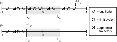
Figure 3: Trajectories of an AS, ordered w.r.t. their minimum channel LLR.

By Theorems V.1 and VI.1, the rightmost bad trajectory is an equilibrium.

The results found so far can be exploited to deactivate many ASs during the decoding process, using two different saturation levels. Without loss of generality we set the saturation level of extrinsic messages equal to $\pm 1$, and the saturation level of channel LLRs equal to $\pm L_{ch}$, with $0<L_{ch}\leq 1$. The latter saturation level defines the range of admissible channel LLRs, depicted in Figs. 3(a) and 3(b) as a gray box. The decoding trajectories within ASs can be very different in case of positive or negative thresholds:

• if $\tau\geq 0$, the saturation of channel LLRs to $\pm L_{ch}$ does not destroy bad trajectories. This is graphically represented in Fig. 3(a);

• if $\tau<0$, we can set $L_{ch}<-\tau=|\tau|$. With this choice, channel LLRs can never lead to bad trajectories, as depicted in Fig. 3(b). Therefore, by Theorem VI.1 the AS is defused.

VII Simulation Results

The behavior of bad structures under iterative decoding in a large code graph is in good agreement with the theory developed so far. For instance, consider the AS (5,3) with topology shown in Fig. 2.

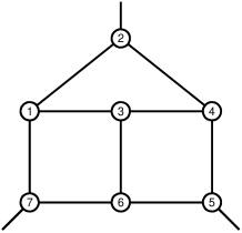
Figure 4: A (7,3) elementary absorbing set.

For this AS, $\tau=-1/3$ (a method to compute thresholds will be presented in the next Section).

In Fig. 5(a) we plot its contribution to the error-floor of an LDPC code having block size $30\,000$ and rate $4/5$.

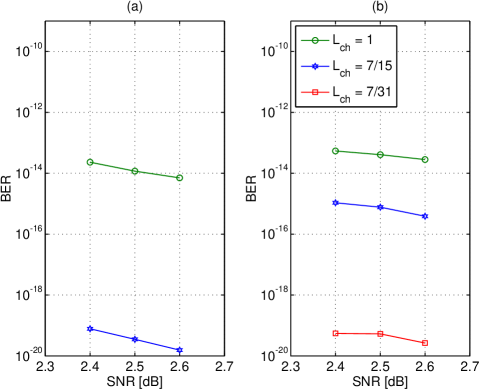
Figure 5: Error floor contributions of the (5,3) and (7,3) ASs shown in Figs. 2 and 4, respectively. The error floors have been obtained applying Importance Sampling to a real LDPC code, under MS sequential decoding.

The simulations are run using Importance Sampling over a Gaussian channel, with SNR around 2.5 dB. We always let the quantized channel LLRs vary in the range $\left[-7,7\right]$, while the extrinsic LLRs are quantized with a varying number $q_{e}$ of bits. Therefore extrinsic messages belong to the interval $\left[-2^{q_{e}-1}+1,2^{q_{e}-1}-1\right]$, and $L_{ch}=\frac{7}{2^{q_{e}-1}-1}$. Decisions are taken after 20 iterations of MS sequential decoding.

From Fig. 5(a) it is apparent that the probability that the MS decoder be locked by the AS is lowered when $L_{ch}$ is reduced from $1$ to $7/15$. However, this is larger than $|\tau|=1/3$ and an error floor still appears. In agreement with the predictions of our theory, if we set $L_{ch}=7/31<|\tau|$ the AS is always unlocked and the error probability is zero.

In Fig. 5(b) we plot the same curves for another AS embedded in the same LDPC code. This AS is shown in Fig. 4 and its $\tau=-1/9$. Once again, reducing $L_{ch}$ decreases the error probability, but now $L_{ch}=7/31$ does not guarantee an error-free performance.

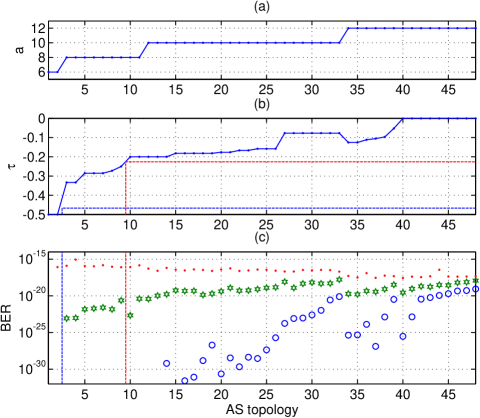
Figure 6: Error floor contributions of 48 ASs, with various channel saturation levels.

Fig. 6 refers to a different code, with the same blocklength and rate. Here we have 48 different AS topologies of size $a=6,8,10,12$ (see Fig. 6(a)), $b=4$, whose thresholds are shown in Fig. 6(b). In Fig. 6(c) we plot the BER contribution of each topology, with various channel saturation levels. The results agree with the predictions of our model. If $L_{ch}=1$, all ASs contribute to the error floor. If $L_{ch}=7/15$ all the (6,4) ASs, whose threshold $\tau=-1/2$, are deactivated. With $L_{ch}=7/31$ all (8,4) ASs below threshold are deactivated. Also some ASs with threshold just above $-7/31$ gave no errors. Besides, Fig. 6(c) shows a good correlation between the thresholds and the dangerousness of the ASs.

VIII A search algorithm for thresholds

VIII-A Towards an affordable linear problem

With the aim of deriving an efficient algorithm to compute the AS threshold, we further simplify Problem IV.1, introducing

Problem VIII.1.

$$\tilde{\tau}=\max_{\lambda,\mathbf{x}} \quad\lambda$$

$$s.t. \quad-\mathbf{1}\leq\mathbf{x}\leq\mathbf{1}$$ (31)

$$\quad\exists j:x_{j}<1$$ (32)

$$\quad\mathbf{x}\geq\mathrm{\widetilde{sat}}\left(\mathbf{A}\left(\mathbf{x}-\mathbf{1}\right)+(2+\lambda)\mathbf{1}\right)$$ (33)

where $\mathrm{\widetilde{sat}}(x)\triangleq\min(x,1)$. With respect to Problem IV.1, only the upper saturation is still present in $\mathrm{\widetilde{sat}}(\cdot)$: extrinsic messages can now assume any negative value. Besides, the constraint imposed by the equilibrium equality has been relaxed, and substituted by an inequality containing only a scalar value $\lambda$. Notwithstanding these modifications, the following theorems hold:

Theorem VIII.1.

As for Problems IV.1 and VIII.1, $\tau^{*}=\tilde{\tau}$.

Proof:

We show that $\tau^{*}\leq\tilde{\tau}$ and $\tau^{*}\geq\tilde{\tau}$.

Assume we are given a solution $(\mathbf{x}^{*},\boldsymbol{\lambda}^{*})$ of Problem IV.1, i.e. with $\min(\boldsymbol{\lambda}^{*})=\tau^{*}$. We can exhibit a pair $(\mathbf{\tilde{x}},\tilde{\lambda})$ that satisfies the constraints of Problem VIII.1. Indeed

$$\mathbf{x}^{*}=\mathrm{sat}\left(\mathbf{A}\left(\mathbf{x}\textsection^{*}-\mathbf{1}\right)+2\cdot\mathbf{1}+\boldsymbol{\lambda}^{*}\right)\\ \geq\mathrm{sat}\left(\mathbf{A}\left(\mathbf{x}^{*}-\mathbf{1}\right)+\left(2+\min(\boldsymbol{\lambda}^{*})\right)\mathbf{1}\right)\\ \geq\mathrm{\widetilde{sat}}\left(\mathbf{A}\left(\mathbf{x}^{*}-\mathbf{1}\right)+\left(2+\min(\boldsymbol{\lambda}^{*})\right)\mathbf{1}\right)\,.$$ (34)

Therefore, the pair $\left(\mathbf{\tilde{x}}=\mathbf{x}^{*},\tilde{\lambda}=\min(\boldsymbol{\lambda}^{*})\right)$ fulfills the constraints of Problem VIII.1, because also $\exists j:\tilde{x}_{j}=x_{j}^{*}<1$. Being $\tilde{\tau}$ the result of a maximization, $\tilde{\tau}\geq\tilde{\lambda}=\min(\boldsymbol{\lambda}^{*})=\tau^{*}$.

Focusing on the converse, assume we are given a solution $(\mathbf{\tilde{x}},\tilde{\lambda})$ of Problem VIII.1, with $\tilde{\lambda}=\tilde{\tau}$. No matter whether extrinsic messages are saturated or not, we can always add a positive vector $\mathbf{\Delta}\geq\mathbf{0}$ to $\tilde{\lambda}\cdot\mathbf{1}$:

$$\mathbf{\Delta}=\mathbf{\tilde{x}}-\mathrm{\widetilde{sat}}\left(\mathbf{A}\left(\mathbf{\tilde{x}}-\mathbf{1}\right)+(2+\tilde{\lambda})\mathbf{1}\right)\,.$$ (35)

This way, we turn inequality (33) into the equality

$$\mathbf{\tilde{x}}=\mathrm{\widetilde{sat}}\left(\mathbf{A}\left(\mathbf{\tilde{x}}-\mathbf{1}\right)+2\cdot\mathbf{1}+\tilde{\lambda}\cdot\mathbf{1}+\mathbf{\Delta}\right)\,.$$ (36)

The constraints of Problem VIII.1 set $\mathbf{x}\geq-\mathbf{1}$, thus we conclude that

$$\mathrm{\widetilde{sat}}\left(\mathbf{A}\left(\mathbf{\tilde{x}}-\mathbf{1}\right)+2\cdot\mathbf{1}+\tilde{\lambda}\cdot\mathbf{1}+\mathbf{\Delta}\right)\geq-\mathbf{1}$$ (37)

and finally

$$\mathrm{\widetilde{sat}}\left(\mathbf{A}\left(\mathbf{\tilde{x}}-\mathbf{1}\right)+2\cdot\mathbf{1}+\tilde{\lambda}\cdot\mathbf{1}+\mathbf{\Delta}\right)\\ =\mathrm{sat}\left(\mathbf{A}\left(\mathbf{\tilde{x}}-\mathbf{1}\right)+2\cdot\mathbf{1}+\tilde{\lambda}\cdot\mathbf{1}+\mathbf{\Delta}\right)\,.$$ (38)

To conclude, if a solution $(\mathbf{\tilde{x}},\tilde{\lambda})$ of Problem VIII.1 with $\tilde{\lambda}=\tilde{\tau}$ exists, we can exhibit a generalized equilibrium $(\mathbf{x}^{*}=\mathbf{\tilde{x}},\boldsymbol{\lambda}^{*}=\tilde{\lambda}\cdot\mathbf{1}+\mathbf{\Delta})$ solution of Problem IV.1, with $\mathbf{\Delta}\geq\mathbf{0}$. Being $\tau^{*}$ the result of a maximization, we conclude that $\tau^{*}\geq\min(\boldsymbol{\lambda}^{*})=\min(\tilde{\lambda}\cdot\mathbf{1}+\mathbf{\Delta})\geq\tilde{\lambda}=\tilde{\tau}$. ∎

Once again, Problems IV.1 and VIII.1 are not equivalent, as the solutions are different (the second one is not even a generalized equilibrium). Anyway, the two thresholds are the same.

Problem VIII.1 is still non-linear and multimodal. Besides, equations are still not differentiable. We further elaborate, rewriting Problem VIII.1 in another form that does not rely on the $\widetilde{\mathrm{sat}}(\cdot)$ function: we define a partition of $\{1,\ldots,N\}$ in the two subsets $\mathcal{S}^{unsat}$ and $\mathcal{S}^{sat}$ of unsaturated and saturated messages, respectively. We also introduce a permutation matrix $\mathbf{\Pi}$, that reorganizes extrinsic messages, putting the unsaturated ones on top:

$$\begin{bmatrix}\mathbf{x}_{\mathcal{S}^{unsat}}\\ \mathbf{1}\\ \end{bmatrix}=\mathbf{\Pi}\mathbf{x}\,.$$ (39)

Accordingly, we permute the routing matrix $\mathbf{A}$, and divide it in four submatrices, having inputs/outputs saturated or not:

$$\mathbf{\Pi}\mathbf{A}\mathbf{\Pi}^{-1}=\begin{bmatrix}\mathbf{A}_{\mathcal{S}^{unsat},\mathcal{S}^{unsat}}&\mathbf{A}_{\mathcal{S}^{unsat},\mathcal{S}^{sat}}\\ \mathbf{A}_{\mathcal{S}^{sat},\mathcal{S}^{unsat}}&\mathbf{A}_{\mathcal{S}^{sat},\mathcal{S}^{sat}}\\ \end{bmatrix}\,.$$ (40)

We are now ready to introduce

Problem VIII.2.

$$\dot{\tau} =\max_{\begin{subarray}{c}\mathcal{S}^{unsat}\subseteq\{1,\ldots,N\}\\ \mathcal{S}^{unsat}\neq\emptyset\end{subarray}}\max_{\lambda,\mathbf{x}_{\mathcal{S}^{unsat}}}\quad\lambda$$

$$s.t. \quad-\mathbf{1}\leq\mathbf{x}_{\mathcal{S}^{unsat}}\leq\mathbf{1}$$ (41)

$$\quad(\mathbf{A}_{\mathcal{S}^{unsat},\mathcal{S}^{unsat}}-\mathbf{I})\left(\mathbf{x}_{\mathcal{S}^{unsat}}-\mathbf{1}\right)+(1+\lambda)\mathbf{1}\leq\mathbf{0}$$ (42)

$$\quad\mathbf{A}_{\mathcal{S}^{sat},\mathcal{S}^{unsat}}\left(\mathbf{x}_{\mathcal{S}^{unsat}}-\mathbf{1}\right)+(1+\lambda)\mathbf{1}\geq\mathbf{0}\,.$$ (43)

Note that the use of $\mathcal{S}^{unsat}$ in the above problem is slightly misleading: even if the outer (leftmost) maximization sets $j\in\mathcal{S}^{unsat}$, thanks to (41) the inner maximization could achieve its maximum even in $x_{j}=1$, and not in $x_{j}<1$. We shall show that this relaxation does not impair the threshold computation.

The following theorem holds.

Theorem VIII.2.

As for Problems VIII.1 and VIII.2, $\tilde{\tau}=\dot{\tau}$.

Proof:

We only give a sketch of the proof, since it is simple but quite long. We show that Problem VIII.1 implies Problem VIII.2, and vice-versa.

First, (32) means that $\mathcal{S}^{unsat}\neq\emptyset$. Rewriting (33) in the modified order, we obtain $\mathbf{x}_{\mathcal{S}^{unsat}}\geq\mathbf{A}_{\mathcal{S}^{unsat},\mathcal{S}^{unsat}}\left(\mathbf{x}_{\mathcal{S}^{unsat}}-\mathbf{1}\right)+(2+\lambda)\mathbf{1}$, since in the first block of inequalities the $\mathrm{\widetilde{sat}}(\cdot)$ operator is useless. Therefore (42) must be true. As for the second block of inequalities, they hold only if the argument of the $\mathrm{\widetilde{sat}}(\cdot)$ exceeds $\mathbf{1}$, i.e., $\mathbf{A}_{\mathcal{S}^{sat},\mathcal{S}^{unsat}}\left(\mathbf{x}_{\mathcal{S}^{unsat}}-\mathbf{1}\right)+(2+\lambda)\mathbf{1}\geq\mathbf{1}$, that immediately leads to (43).

Analogous arguments hold for the converse. The only tricky point is the following. Let $(\mathbf{\dot{x}},\dot{\lambda})$ be a maximizer for Problem VIII.2, with $\dot{\lambda}=\dot{\tau}$, and $\mathcal{\dot{S}}^{unsat}$ the set corresponding to this solution. As already highlighted, $\mathcal{\dot{S}}^{unsat}$ could contain indices referring to saturated variables. If at least one element of $\mathbf{x}_{\mathcal{\dot{S}}^{unsat}}$ is not saturated, this does not impair the outer maximization, since the same solution $(\mathbf{\dot{x}},\dot{\lambda})$ is a maximizer with another pattern of saturations $\mathcal{S}^{unsat}=\left\{j\in\mathcal{\dot{S}}^{unsat}:\dot{x}_{j}<1\right\}\neq\emptyset$. In this case, (32) is satisfied. On the contrary, if all messages in $\dot{S}^{unsat}$ were saturated, we could achieve the maximum $\lambda$ not respecting (32), obtaining $\dot{\tau}\geq\tilde{\tau}$. We now prove that this cannot happen. Indeed, if we set $\mathbf{x}_{\mathcal{S}^{unsat}}=\mathbf{1}$, (42) becomes $\lambda\leq-1$. Yet, similarly to Theorem III.1, there are always other legitimate solutions having $\lambda=-1$ that do not violate the constraints of Problem VIII.2, e.g. $\left(\mathbf{x}=-\mathbf{1},\lambda=-1\right)$, for which (43) has no meaning and (42) becomes $-2(\mathbf{A}-\mathbf{I})\mathbf{1}\leq\mathbf{0}$, that is true because $\mathbf{A}\mathbf{1}\geq\mathbf{1}$. We conclude that $\dot{\tau}\geq-1$ and that substituting $\mathbf{x}_{\mathcal{S}^{unsat}}<\mathbf{1}$ with $\mathbf{x}_{\mathcal{S}^{unsat}}\leq\mathbf{1}$ does not harm the threshold computation. ∎

Once again, we do not distinguish any more between $\tau^{\prime}$, $\tau^{*}$, $\tilde{\tau}$ and $\dot{\tau}$ since they match, and simply use $\tau$.

In principle, we could solve the inner maximization of Problem VIII.2, repeatedly running an optimization algorithm suited to linear equality and inequality constraints (e.g., the simplex algorithm), and retaining only the largest value of $\tau$ among all possible configurations of saturated messages. This is practically unfeasible for two reasons. First, optimization algorithms are time-consuming and we should resort to them with caution. Besides, the number of configurations to test grows exponentially with $N$. Solving Problem VIII.2 with a brute-force search becomes unpracticable even for moderate values of $N$. In the following, we develop methods to discard most $\mathcal{S}^{unsat}$ configurations.

VIII-B Pruning tests

Test 1 exploits the following two theorems:

Theorem VIII.3.

If $\mathbf{A}_{\mathcal{S}^{unsat},\mathcal{S}^{unsat}}$ contains at least one row with all-zero elements, there are no solutions satisfying the constrains of Problem VIII.2.

Proof:

The proof is a reductio ad absurdum. Consider any row of $\mathbf{A}_{\mathcal{S}^{unsat},\mathcal{S}^{unsat}}$ with null weight, say the one corresponding to the $j$-th in $\mathbf{x}$. Then, by (42),

$$x_{j}\geq 2+\lambda\geq 1$$ (44)

where the second inequality holds since $\lambda\geq-1$. The above result $x_{j}\geq 1$ contradicts the hypothesis $j\in\mathcal{S}^{unsat}$ . ∎

Theorem VIII.4.

If $\mathbf{A}_{\mathcal{S}^{unsat},\mathcal{S}^{unsat}}$ contains at least one row with exactly one element equal to $1$, say $A_{j,h}$, and if the column vector $\mathbf{A}_{\mathcal{S}^{sat},h}$ has weight larger than $0$, then there are no solutions satisfying the constraints of Problem VIII.2.

Proof:

The proof is a reductio ad absurdum. Consider any non null element of $\mathbf{A}_{\mathcal{S}^{sat},h}$, say $A_{i,h}$. Note that the maximum weight of any row and column of $\mathbf{A}$ is 2, being the VN degree $d=3$. Thus, either $A_{i,h}$ is the only non-null element of the row $\mathbf{A}_{i,\mathcal{S}^{unsat}}$, or at most another element $A_{i,k}=1$ exists in $\mathbf{A}_{i,\mathcal{S}^{unsat}}$. If $\mathbf{A}_{i,\mathcal{S}^{unsat}}$ has weight 1, by (43)

$$1\leq x_{h}-1+2+\lambda=x_{h}+1+\lambda\,.$$ (45)

If $\mathbf{A}_{i,\mathcal{S}^{unsat}}$ has weight 2, by (43)

$$1\leq x_{h}-1+x_{k}-1+2+\lambda\leq x_{h}+1+\lambda$$ (46)

where the second inequality holds since $x_{k}\leq 1$. In either case,

$$x_{j}\geq x_{h}-1+2+\lambda\geq 1$$ (47)

where the first inequality comes from (42). The above result $x_{j}\geq 1$ contradicts the hypothesis $j\in\mathcal{S}^{unsat}$ . ∎

Theorems VIII.3 and VIII.4 suggest sufficient conditions to discard configurations of $\mathcal{S}^{unsat}$. The advantage of Test 1 is simplicity. The weakness of Test 1 is that it does not take advantage of previous maximizations, with other configurations of $\mathcal{S}^{unsat}$.

Test 2 exploits the threshold $\tau$ discovered up to that time. It starts initializing lower and upper bounds ($\mathbf{l}$ and $\mathbf{u}$, respectively) for the minimum channel LLR $\lambda$ and for $\mathbf{x}_{\mathcal{S}^{unsat}}$:

$$\mathbf{l}\leq\begin{bmatrix}\lambda\\ \mathbf{x}_{\mathcal{S}^{unsat}}\\ \end{bmatrix}\leq\mathbf{u}$$ (48)

where

$$\mathbf{l}=\begin{bmatrix}\tau\\ -\mathbf{1}_{M\times 1}\end{bmatrix},\quad\quad\quad\mathbf{u}=\begin{bmatrix}\lambda_{max}\\ \mathbf{1}_{M\times 1}\end{bmatrix}$$ (49)

and $M=\mathrm{card}\left(\mathcal{S}^{unsat}\right)$. In the most general case, $\lambda_{max}=1$. Yet we are mainly interested in the negative semi-axis, since in Section VI we have shown that we can deactivate an AS only if the threshold is negative. Therefore, in the threshold computation algorithm we can lower $\lambda_{max}$ (of course, we must keep $\lambda_{max}\geq 0$), exchanging some information loss (we return $\min(\tau,\lambda_{max})=\lambda_{max}$ when $\tau>\lambda_{max}$), for an increased capability to discard saturation patterns, resulting in an execution speedup.

Test 2 analyzes the inequality constraints of Problem VIII.2 in turn, rewritten as

$$\mathbf{C}\begin{bmatrix}\lambda\\ \mathbf{x}_{\mathcal{S}^{unsat}}\\ \end{bmatrix}\leq\mathbf{f}$$ (50)

with

$$\mathbf{C} = \begin{bmatrix}\mathbf{1}_{M\times 1}&\mathbf{A}_{\mathcal{S}^{unsat},\mathcal{S}^{unsat}}-\mathbf{I}\\ -\mathbf{1}_{(N-M)\times 1}&-\mathbf{A}_{\mathcal{S}^{sat},\mathcal{S}^{unsat}}\\ \end{bmatrix}$$ (51)

$$\mathbf{f} = \begin{bmatrix}\mathbf{A}_{\mathcal{S}^{unsat},\mathcal{S}^{unsat}}\mathbf{1}_{M\times 1}-2\cdot\mathbf{1}_{M\times 1}\\ \mathbf{1}_{(N-M)\times 1}-\mathbf{A}_{\mathcal{S}^{sat},\mathcal{S}^{unsat}}\mathbf{1}_{M\times 1}\\ \end{bmatrix}\,.$$ (52)

For every variable involved, the test tries to tighten the gap between the corresponding lower and upper bounds, exploiting bounds (upper or lower, depending on the coefficient signs) on the other variables. The process can terminate in two ways:

1. bounds $\mathbf{l}$ and $\mathbf{u}$ cannot be further improved, and $\mathbf{l}\leq\mathbf{u}$: $\tau$ and $\mathcal{S}^{unsat}$ are compatible with the existence of other equilibria, having thresholds larger than $\tau$;

2. for at least one index $j$, we achieve $u_{j}<l_{j}$: equilibria having thresholds larger than the currently discovered $\tau$ cannot exist, for that $\mathcal{S}^{unsat}$.

The initialization in (49) influences the algorithm effectiveness: the more the discovered threshold $\tau$ gets large, the more Test 2 will effectively detect impossible configurations of $\mathcal{S}^{unsat}$, speeding up the solution of Problem VIII.2.

VIII-C Tree based, efficient search of the AS threshold

Test 2 is typically more effective than Test 1, as it can detect a large number of configurations of $\mathcal{S}^{unsat}$ not improving the threshold $\tau$. Yet, it can be applied only when $\mathcal{S}^{unsat}$ is formed. On the contrary, Test 1 can also be applied during the construction of $\mathcal{S}^{unsat}$:

Theorem VIII.5.

Let $\mathcal{S}^{violation}\subseteq\mathcal{S}^{unsat}$ be the set of indices satisfying Theorems VIII.3 or VIII.4. Erasing only a subset of $\mathcal{S}^{violation}$ from $\mathcal{S}^{unsat}$, the other elements in $\mathcal{S}^{violation}$ still satisfy conditions of Theorems VIII.3 or VIII.4.

Proof:

Assume that only one element involved in some violation, say the $m$-th, is erased by $\mathcal{S}^{unsat}$. The proof for a generic subset of violations, erased all together, can be achieved repeating the following argument many times, discarding one element after the other.

When element $m$ passes from $\mathcal{S}^{unsat}$ to $\mathcal{S}^{sat}$, not only the row $\mathbf{A}_{m,\mathcal{S}^{unsat}}$ must be erased, but also the column $\mathbf{A}_{\mathcal{S}^{unsat},m}$ must be canceled. Looking at any other row of $\mathbf{A}_{\mathcal{S}^{unsat},\mathcal{S}^{unsat}}$ leading to a violation, say the one corresponding to element $j$, three events can happen (see Fig. 7):

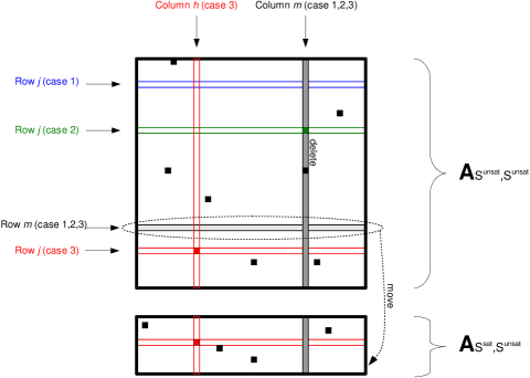
Figure 7: Row-column erasure possibilities in $\mathbf{A}_{\mathcal{S}^{unsat},\mathcal{S}^{unsat}}$.

1. $\mathbf{A}_{j,\mathcal{S}^{unsat}}$ had weight 0: after column deletion, it still has weight 0 and the hypothesis of Theorem VIII.3 is still valid;

2. $\mathbf{A}_{j,\mathcal{S}^{unsat}}$ had weight 1, and its element equal to 1 was exactly in the $m$-th column (the erased one): after deletion, the row assumes weight 0, therefore satisfying the hypothesis of Theorem VIII.3;

3. $\mathbf{A}_{j,\mathcal{S}^{unsat}}$ had weight 1, and the element equal to 1, say $A_{j,h}$ did not lie in the $m$-th column: after deletion, the row of $\mathbf{A}_{\mathcal{S}^{unsat},\mathcal{S}^{unsat}}$ still has weight 1. Since the weight of the corresponding column $\mathbf{A}_{\mathcal{S}^{sat},h}$ is still 1 (it had weight 1 by hypothesis), Theorem VIII.4 still holds for the $j$-th element.

Either Theorem VIII.3 or VIII.4 are still valid, and the other violations do not disappear. ∎

The above Theorem gives us the freedom to erase elements in $\mathcal{S}^{violation}$ all together from $\mathcal{S}^{unsat}$, and simultaneously add them to $\mathcal{S}^{sat}$. Therefore, we can imagine a tree search among all possible configurations of saturated messages.

At the root node, $\mathcal{S}^{sat}=\emptyset$. At successive steps, some extrinsic messages are marked as already visited (“fixed”, from here on). In addition, fixed messages are labeled as saturated or not. Extrinsic messages not fixed (say “free”) are always unsaturated. This implicitly defines $\mathcal{S}^{sat}$ and $\mathcal{S}^{unsat}$. For the current configuration, Test 1 is performed. Three things can happen:

• Case 1: Test 1 claims that Problem VIII.2 may have solutions for that $\mathcal{S}^{sat}$;

• Case 2: Test 1 claims that $\mathcal{S}^{sat}$ is incompatible with any solution of Problem VIII.2, and all the elements generating a test violation are free;

• Case 3: Test 1 claims that $\mathcal{S}^{sat}$ is incompatible with any solution of Problem VIII.2, but some elements generating a test violation have been previously fixed (and marked as unsaturated).

Depending on the answer of Test 1, we expand the tree in different manners:

• in Case 1, in turn we fix one of the free messages, and branch the tree, labeling the last element as either saturated or not, calling the algorithm recursively;

• in Case 2, we fix and mark as saturated all elements of $\mathcal{S}^{unsat}$ that generate violations, and call the algorithm recursively;

• in Case 3, or if all variables have been already fixed, we take no action.

After Test 1, before the tree branching, we either perform optimization or not:

• in Case 1 or 2, Test 2 is executed. In case of negative result, we return $\tau=-1$; otherwise, the simplex algorithm is eventually performed to solve Problem VIII.2 for the current $\mathcal{S}^{unsat}$;

• in Case 3, we return the partial result $\tau=-1$.

This way, Test 1 speeds up the construction of $\mathcal{S}^{sat}$ and prunes many branches. Test 2 avoids the execution of the simplex algorithm for many useless configurations, not detected by Test 1.

IX Additional properties

IX-A Punctured LDPC codes

Puncturing is a popular means to adapt the code rate or even achieve rate compatibility [17]. An interesting extension of our theory is that harmless ASs having $\tau<-L_{ch}$ are deactivated even in case of puncturing.

Theorem IX.1.

Puncturing at most $a-1$ VNs of an AS does not increase the threshold.

Proof:

Assume that an AS $(a,b)$ of threshold $\tau$ is punctured in less than $a$ VNs. Let $\boldsymbol{\lambda}^{p}$ be the set of channel LLRs, with null messages for the punctured VNs. First, consider the case $\tau<0$. Assume that after puncturing, a bad trajectory $\{\mathbf{x}^{(k)}\}$ exists, with $\min(\boldsymbol{\lambda}^{p})>\tau$. This is an absurdum, since $\boldsymbol{\lambda}^{p}$ is a legitimate solution without puncturing, and the definition of threshold given e.g. in Problem III.1 is contradicted. This holds as long as at least one variable is not punctured, otherwise nothing is left to optimize and $\boldsymbol{\lambda}^{p}=\mathbf{0}>\tau\cdot\mathbf{1}$.

Consider now the case $\tau\geq 0$. Since at least one entry of $\boldsymbol{\lambda}^{p}$ is equal to $0$, we have $\min(\boldsymbol{\lambda}^{p})\leq 0$. Thus $\min(\boldsymbol{\lambda}^{p})\leq\tau$ and the threshold of the same AS without puncturing is not exceeded. ∎

Therefore, ASs having $\tau<-L_{ch}$ cannot become harmful.

IX-B Thresholds are rational numbers

A final, not trivial property of thresholds is the following.

Theorem IX.2.

Thresholds $\tau\in\mathbb{Q}$.

Proof:

We focus on Problem VIII.2. We will prove the theorem for any constrained saturation pattern $S^{unsat}$. Therefore, the result will hold for the maximum across all possible $S^{unsat}$. The proof is slightly cumbersome, and involves standard concepts of linear programming theory.

First, note that constraints $-\mathbf{1}\leq\mathbf{x}\leq\mathbf{1}$ bound the feasible space of extrinsic messages. By Theorem III.1, the constraint $-1\leq\lambda\leq 1$ can be added without modifying the result. Therefore, the above constraints and the others in Problem VIII.2 define a polytope $\mathcal{P}$ in $M+1$ dimensions

$$\mathbf{y}\in\mathcal{P}\Longleftrightarrow\underbrace{\begin{bmatrix}\mathbf{I}_{(M+1)\times(M+1)}\\ -\mathbf{I}_{(M+1)\times(M+1)}\\ \mathbf{C}\\ \end{bmatrix}}_{\triangleq\mathbf{C}^{\prime}}\mathbf{y}\leq\underbrace{\begin{bmatrix}\mathbf{1}_{(M+1)\times 1}\\ \mathbf{1}_{(M+1)\times 1}\\ \mathbf{f}\\ \end{bmatrix}}_{\triangleq\mathbf{f}^{\prime}}$$ (53)

where

$$\mathbf{y}\triangleq\begin{bmatrix}\lambda\\ \mathbf{x}_{\mathcal{S}^{unsat}}\\ \end{bmatrix}$$ (54)

Geometrically, the above inequality constraints reported in canonical form represent half-spaces that “shave” the polytope. The polytope $\mathcal{P}$ is convex, since it results from the intersection of half-spaces, that are affine and therefore convex. To conclude, our optimization problem can be re-stated as

$$\max_{\mathbf{y}}\;\mathbf{w}^{T}\mathbf{y},\quad\quad s.t.\quad\mathbf{y}\in\mathcal{P}$$ (55)

with $\mathbf{w}=\begin{bmatrix}1&0&\ldots&0\\ \end{bmatrix}^{T}$. Our feasible region cannot be empty, since we already know that a solution $(\lambda=-1,\mathbf{x}_{\mathcal{S}^{unsat}}=-\mathbf{1})$, i.e. $\mathbf{y}=-\mathbf{1}$ always exists.

From Linear Programming Theory [18], we know that the number of independent constraints at any vertex is $M+1$ and that at least one vertex is an optimizer in linear programming problems (the latter part is the enunciation of the Fundamental Theorem of Linear Programming).

Focus on a vertex $\mathbf{v}$ that is also a maximizer, and on the $M+1$ linearly independent constraints satisfied with equality in that point. Let $\mathcal{A}$ be the set of these constraints. We can write $\mathbf{C}^{\prime}_{\mathcal{A},\{1,\ldots,M+1\}}\mathbf{v}=\mathbf{f}^{\prime}_{\mathcal{A}}$. Being $\mathbf{C}^{\prime}_{\mathcal{A},\{1,\ldots,M+1\}}$ full-rank, we can achieve a full QR-like decomposition $\mathbf{C}^{\prime}_{\mathcal{A},\{1,\ldots,M+1\}}=\mathbf{Q}\mathbf{L}$, being $\mathbf{Q}$ orthogonal, and $\mathbf{L}$ lower triangular. Note that, being the entries of $\mathbf{C}^{\prime}_{\mathcal{A},\{1,\ldots,M+1\}}$ rational (actually, integer), we can always keep the elements of $\mathbf{Q}$ and $\mathbf{L}$ rational, e.g. performing a Gram-Schmidt decomposition. Multiplying both sides of the above equation by $\mathbf{Q}^{T}$, we obtain

$$\mathbf{L}\mathbf{v}=\mathbf{Q}^{T}\mathbf{f}^{\prime}_{\mathcal{A}}\,.$$ (56)

Focusing on the first line of the above system, we achieve $v_{1}=\lambda\in\mathbb{Q}$, since also $\mathbf{f}^{\prime}\in\mathbb{Q}$. ∎

X Conclusions

In this paper we defined a simplified model for the evolution inside an absorbing set of the messages of an LDPC Min-Sum decoder, when saturation is applied. Based on this model we identified a parameter for each AS topology, namely a threshold, that is the result of a max-min non linear problem, for which we proposed an efficient search algorithm. We have shown that based on this threshold it is possible to classify the AS dangerousness. If all the channel LLRs inside the AS are above this threshold, after a sufficient number of iterations the MS decoder can not be trapped by the AS.

Future work will primarily focus on the extension of these concepts to scaled and offset MS decoders. We are also trying to further simplify the threshold evaluation.

References

- [1] B. J. Frey, R. Koetter, and A. Vardy, “Signal-space characterization of iterative decoding,” IEEE Trans. Inf. Theory, vol. 47, no. 2, pp. 766–781, Feb. 2001.
- [2] R. Koetter and P. . Vontobel, “Graph covers and iterative decoding of finite-length codes,” in International Symposium on Turbo Codes & Related Topics, Brest, France, Sept. 2003, pp. 75–82.
- [3] T. Richardson, “Error floors of LDPC codes,” in Annual Allerton Conf. on Commun., Contr. and Computing,, Oct. 2003, pp. 1426–1435.
- [4] S. Chilappagari, S. Sankaranarayanan, and B. Vasic, “Error Floors of LDPC Codes on the Binary Symmetric Channel,” in IEEE International Conference on Communications (ICC’06), Istanbul, Turkey, June 2006, pp. 1089–1094.
- [5] S. Chilappagari, M. Chertkov, M. Stepanov, and B. Vasic, “Instanton-based techniques for analysis and reduction of error floors of LDPC codes,” IEEE J. Select. Areas Commun., vol. 27, no. 6, pp. 855–865, June 2009.
- [6] L. Dolecek, Z. Zhang, M. Wainwright, V. Anantharam, and B. Nikolic, “Analysis of absorbing sets for array-based LDPC codes,” in IEEE International Conference on Communications (ICC’07), Glasgow, Scotland, U.K., June 2007, pp. 6261–6268.
- [7] L. Dolecek, P. Lee, Z. Zhang, V. Anantharam, B. Nikolic, and M. Wainwright, “Predicting error floors of structured LDPC codes: deterministic bounds and estimates,” IEEE J. Select. Areas Commun., vol. 27, no. 6, pp. 908–917, Aug. 2009.
- [8] Z. Zhang, L. Dolecek, B. Nikolic, V. Anantharam, and M. Wainwright, “Design of LDPC decoders for improved low error rate performance: quantization and algorithm choices,” IEEE Trans. Wireless Commun., vol. 57, no. 11, pp. 3258–3268, Nov. 2009.
- [9] C. Schlegel, “On the dynamics of the error floor behavior in (regular) LDPC codes,” IEEE Trans. Inf. Theory, vol. 56, no. 7, pp. 3248–3264, July 2010.
- [10] L. Dolecek, Z. Zhang, V. Anantharam, M. Wainwright, and B. Nikolic, “Analysis of absorbing sets and fully absorbing sets of array-based LDPC codes,” IEEE Trans. Inf. Theory, vol. 56, no. 1, pp. 181–201, Jan. 2010.
- [11] Z. Zhang, L. Dolecek, B. Nikolic, V. Anantharam, and W. M., “Lowering LDPC error floors by postprocessing,” in GLOBECOM 2008, New Orleans, LA, Dec. 2008, pp. 1–6.
- [12] J. Sun, O. Y. Takeshita, and M. P. Fitz, “Analysis of trapping sets for LDPC codes using a linear system model,” in Annual Allerton Conf. on Commun., Contr. and Computing,, Oct. 2004.
- [13] B. Butler and P. Siegel, “Error floor approximation for LDPC codes in the AWGN channel,” in Annual Allerton Conf. on Commun., Contr. and Computing,, Oct. 2011, pp. 204–211.
- [14] L. Dolecek, “On absorbing sets of structured sparse graph codes,” in Information Theory and Applications Workshop (ITA), UCSD, San Diego, CA, Feb. 1-5 2010, pp. 1–5.
- [15] D. MacKay and M. Postol, “Weaknesses of Margulis and Ramanujan-Margulis low-density parity-check codes,” Electron. Notes in Theor. Comp. Sci., vol. 74, no. 10, pp. 97–104, Oct. 2003.
- [16] E. Sharon and J. G. S. Litsyn, “Efficient serial Message-Passing schedules for LDPC decoding,” IEEE Trans. Inf. Theory, vol. 53, no. 11, pp. 4076–4091, Nov. 2007.
- [17] H. Pishro-Nik and F. Fekri, “Results on punctured Low-Density Parity-Check codes and improved iterative decoding techniques,” IEEE Trans. Inf. Theory, vol. 53, no. 2, pp. 599–614, Feb. 2007.
- [18] K. G. Murty, Linear programming. New York: John Wiley & Sons, 1983.