Taking one charge off a two-dimensional Wigner crystal

Abstract

A planar array of identical charges at vanishing temperature forms a Wigner crystal with hexagonal symmetry. We take off one (reference) charge in a perpendicular direction, hold it fixed, and search for the ground state of the whole system. The planar projection of the reference charge should then evolve from a six-fold coordination (center of a hexagon) for small distances to a three-fold arrangement (center of a triangle), at large distances $d$ from the plane. The aim of this paper is to describe the corresponding non-trivial lattice transformation. For that purpose, two numerical methods (direct energy minimization and Monte Carlo simulations), together with an analytical treatment, are presented. Our results indicate that the $d=0$ and $d\to\infty$ limiting cases extend for finite values of $d$ from the respective starting points into two sequences of stable states, with intersecting energies at some value $d_{t}$; beyond this value the branches continue as metastable states.

1 Introduction

In 1934, Wigner Wigner34 pointed out a possible crystallization of a three-dimensional (3D) quantum jellium (one-component plasma), consisting of charged particles immersed in a homogeneous neutralizing background, at low densities. The possibility of the formation of a two-dimensional (2D) crystal of electrons on the surface of liquid helium and in inversion layers of semiconductors at low temperatures was predicted theoretically in Refs. Crandall71 and Chaplik72 , respectively. The corresponding experiments of an electron gas trapped at the surface of liquid helium was realized by Grimes and Adams Grimes79 , in the semiconductor structure GaAs/GaAlAs by Andrei et al. Andrei88 , and of laser-cooled ⁹Be⁺ ions confined in Penning traps by Mitchell et al. Mitchell:98 . For reviews about classical and quantum Coulomb crystals, see e.g. Bonitz08 ; Monarkha12 ; Monarkha:book:03 .

From a theoretical point of view, the ground-state energies of a classical 2D electron crystal and the phonon spectra were studied for a variety of Bravais lattices in Refs. Platzman74 ; Bonsall77 , with the conclusion that a simple hexagonal structure (built up by equilateral triangles) provides the lowest energy. To understand the thermodynamics and the dynamical properties of electrons at low temperatures, deviations from a perfect crystal have been studied in the seminal work of Fisher et al. Fisher79 . These investigations involve (i) localized low-energy defects (such as vacancies, interstitials, etc.) which are expected to govern dynamical properties of migrating electrons, and (ii) extended defects with higher energies (such as dislocations, grain boundaries, etc.) which are supposed to play an important role in the melting process of the crystal. At the present stage of knowledge, grain boundaries are responsible for melting 3D Wigner crystals, while the Kosterlitz-Thouless theory of dislocations and disclinations Kosterlitz73 ; Nelson79 describes the melting of 2D electron crystals. Related models involve curved geometries Messina1 ; Messina2 , large 2D Coulomb clusters confined by a harmonic potential Bedanov94 ; Kong03 , 2D colloidal crystals with pair interactions of Yukawa Libal07 ; He13 or $1/r^{3}$ Lechner09 ; Teeffelen13 forms.

In the present paper, we study from a classical perspective the ground-state problem of taking off a charge from a bidimensional crystal. Our starting point is a perfect, 2D Wigner crystal which we assume to be embedded in the $(x,y)$-plane. It is formed by particles (each with a negative elementary charge of $-e$), localized at the sites of a hexagonal lattice (with lattice spacing $a$). The charges of the particles are neutralized by a uniform background of charge density $\sigma e$. Then, we take one of the charges (carrying the index $0$, and coined the “reference” or “tagged” particle) away from the crystal and fix it at a distance $d$ in the vertical $z$-direction. As we consider increasingly large values for $d$, the remaining particles in the Wigner crystal will leave their original, regular lattice positions and will intuitively approach the vacancy left behind by the tagged particle. This spatial deformation is realized in an effort to minimize the total interaction energy of the setup (i.e., “Wigner crystal + tagged charge”). It stands to reason that the removal of charge 0 has a stronger impact on the particle positions of the lattice the closer these particles have been to the tagged charge in the original Wigner crystal (i.e. at $d=0$). However, one should not forget that due to the long-range nature of the Coulomb potential, the interactions between all particles are important. Two limiting cases can be envisioned. (i) When $d=0$, and presumably when $d/a\ll 1$, the reference particle has coordination six, see Figure 1. (ii) On the other hand, at asymptotically large distances (i.e., for $d/a\gg 1$), the Wigner crystal is interacting only weakly with the tagged particle and therefore the perfect hexagonal structure of the lattice should be maintained. Under these conditions, the total optimal configuration is realized when the projection of the reference particle coincides with the center of any triangle formed by three neighbouring particles of the Wigner crystal (see right panel of Figure 1). The transformation of the Wigner crystal from a six-fold coordination (valid at least for $d=0$) to a three-fold coordination (valid at least for $d\to\infty$), induced by a change in the distance $d$ of the tagged particle, represents the central topic of this contribution.

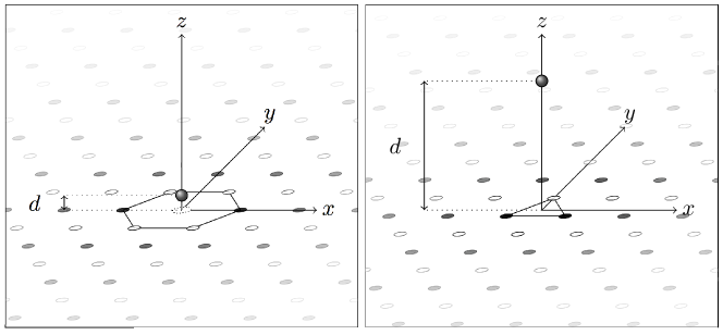
Figure 1: Schematic representation of the two limiting configurations expected. Left panel: When the reference charge is close to the plane, its perpendicular projection is endowed with six-fold coordination. Right panel: at large distances $d$, its coordination number becomes three. In the remainder, the dimensionless counterpart of $d$ will be denoted $\eta$.

To the best of our knowledge, the proposed problem has not been addressed so far. It naturally appears when studying the strong-coupling regime of counter-ions close to a uniformly charged wall Netz01 ; Samaj11 . It also is of relevance within the context of phenomena such as evaporation of particles from a surface at low temperatures or the creation of lattice defects by manipulating individual particles Pertsinidis01a ; Pertsinidis01b . Several fundamental questions arise:

• Does the six-fold coordination of the tagged charge change to a three-fold coordination (or even to some other value) at a finite distance $d_{t}$ or already at an infinitesimally small value?

• What is the nature of the transition as the six-fold coordination is lost? In particular, is it continuous, i.e. do the six nearest neighbours of the tagged particle rearrange in a continuous fashion into some non-equivalent subsets of particles, each specified by a different shift away from their original crystal positions? Or is the transition discontinuous, accompanied by a change in the slope of the energy at the transition distance, $d_{t}$?

• If the three- and six-fold coordinated limiting states lead to metastable configurations at finite $d$, what is the corresponding energy barrier? Does it take a finite value, or does it scale with the number of particles, $N$?

The last question is relevant in view of practical realization of the “experiment”, and also pertinent for computational purposes. Our analysis will show that metastable states can coexist for all distances, separated by an energy barrier that seems high enough so that the system will stay in a local energy minimum also after crossing the transition distance $d_{t}$. In that case, when increasing $d$, one observes a hysteresis similar to that of ferromagnetic systems. In the ferromagnetism of two macroscopic $+$ and $-$ magnetized states, one needs a relatively large opposite magnetic field to reverse the magnetization of a macroscopic domain. In our problem, the role of the magnetic field is taken over by the distance $d$: if $d\gg d_{t}$, the local minimum (a reminiscence of the six-fold coordinated state at $d=0$) might become unstable, or might start to transform into a precursor of the state with three-fold coordination.

The metastability feature will lead us to define two branches (see Section 2): the “out”-branch (extrusion) where $d$ increases, starting from 0 where the coordination is six-fold, and the “in”-branch (intrusion), starting from large $d$ where the coordination number is three, and decreasing $d$ down to 0. It should be kept in mind that we shall consider a sequence of equilibrium situations only, at vanishing temperature (i.e. we let the system find the lowest total energy configuration, for every $d$). In doing so, we will answer a few of the questions addressed above. We have used three theoretical tools: energy minimization, Monte Carlo simulations (both methods being purely numerical), and an analytic approach. They all bear their own limitations, since simplifying assumptions were made to allow for solutions: in both numerical approaches we have considered a unit cell (containing a sufficient number of particles) that contains a finite section of the Wigner crystal as well as the tagged charge; for a fixed position of charge 0, all particles of the remaining lattice are allowed to freely relax their position [remaining in the same $(x,y)$ plane]. The entire system is then a periodic replication of this unit cell. In the analytic approach, the system is assumed to be of infinite extent in the $(x,y)$-direction; however, spatial relaxations were allowed only for the nearest neighbours of the tagged charge, for simplicity.

The manuscript is organized as follows. The model is specified in detail in Section 2, where the two branches are introduced. We then present in Section 3 the basic features of our two numerical approaches, energy minimization and Monte Carlo simulations. Both methods rely on Ewald summation techniques, to take due account of the long range nature of the interaction potential. The analytic approach is presented in Section 4, and the results are subsequently discussed in Section 5. The paper closes with our conclusions and outlook on future work in Section 6. An Appendix collects cumbersome expressions required for the analytic treatment.

2 The system and the two branches protocol

2.1 Definition of the model

Figure 2: Hexagonal structure of the undistorted 2D Wigner crystal, as obtained for $d=0$ or $d\to\infty$. The arrows show $\bm{a}_{1}=\bm{b}_{1}$ and $\bm{a}_{2}$, the primitive lattice vectors defined in Equation (2), while $\bm{b}_{2}$ is defined in Equation (3). Black and white colors are for alternating rows.

We start from the hexagonal structure of the 2D Wigner crystal: its unit cell is a rhombus defined via the primitive lattice vectors

$${\bm{a}}_{1}=a(1,0),\qquad{\bm{a}}_{2}=\frac{a}{2}(1,\sqrt{3}),$$ (1)

where $a$ is the lattice spacing (see Figure 2). The positions in the 2D lattice,

$${\bf R}_{j}=(R_{j}^{x},R_{j}^{y})=j_{1}\,\bm{a}_{1}+j_{2}\,\bm{a}_{2}$$ (2)

are indexed by $j=(j_{1},j_{2})$, where $j_{1}$ and $j_{2}$ are arbitrary integers. Due to the single-occupancy of our crystal, we can use $j$ as the particle index. There exists another, equivalent representation of the hexagonal structure. Let us label the particles along rows alternately with white and black colour. In doing so, we obtain two identical, rectangular sub-lattices (’white’ and ’black’), each of them defined via orthogonal translational vectors

$$\bm{b}_{1}\equiv\bm{a}_{1}=a(1,0),\qquad\bm{b}_{2}=a(0,\sqrt{3}),$$ (3)

see Figure 2. The two sub-lattices are shifted with respect to each another by the vector ${\bm{a}}_{2}=(\bm{b}_{1}+\bm{b}_{2})/2$. This representation is useful when evaluating Coulomb lattice sums (see Section 4).

Let $S$ denote the surface of a finite section of the 2D Wigner crystal formed by $N$ particles. We shall take the limit $S$ (and thus $N$) $\to\infty$, and the electro-neutrality condition imposes that the charge density, $\sigma e$, is given by

$${\sigma=\frac{N}{S}}.$$ (4)

There is exactly one particle per rhombus of surface $\sqrt{3}a^{2}/2$; thus

$$\frac{S}{N}=\frac{\sqrt{3}}{2}a^{2},\qquad\mbox{i.e.}\qquad\frac{\sqrt{3}}{2}a^{2}\sigma=1.$$ (5)

The Coulomb interaction energy of two particles separated by a distance $r$ is given by $e^{2}/r$. The ground-state energy, $E_{0}$, of an infinitely large system (consisting of the hexagonally arranged particles and the neutralising background) is found to be Bonsall77

$$\lim_{N\to\infty}\frac{E_{0}}{N}=\frac{1}{2}\sum_{i,j=-\infty\atop(i,j)\neq(0,0)}^{\infty}\frac{e^{2}}{\sqrt{(ai+\frac{1}{2}aj)^{2}+(\frac{\sqrt{3}}{2}aj)^{2}}}-\mbox{background}=ce^{2}\sqrt{\sigma},$$ (6)

the prefactor $c=-1.960515789319\ldots$ being known as the Madelung constant.

2.2 The “in”- and “out”-branches

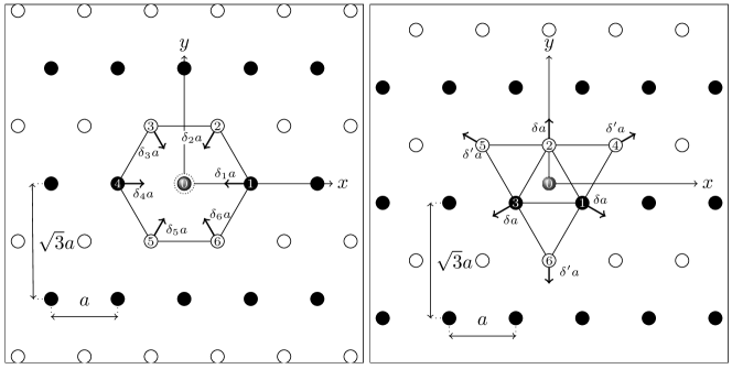
Figure 3: Typical configurations along the two branches, together with labeling of neighbours (from 1 to 6) and their displacements. The tagged charge carries the label 0 and its projection is shown in grey. Left panel: schematic picture along the “out”-branch. Arrows indicate possible displacements ($\delta_{1}a$ to $\delta_{6}a$) of particles 1 to 6, induced by the removal of the tagged particle. Right panel: same, along the “in”-branch. Arrows indicate possible displacements ($\delta a$ for the nearest neighbours and $\delta^{\prime}a$ for the next-nearest neighbours) of particles 1 to 6, induced by the presence of the tagged particle.

As alluded to above, locally stable configurations may be found for a given $d$, which in turn complicates the search for the ground-state of the system. These states seem to be remnants of the coordination six structure valid at $d=0$ on the one hand, and of the coordination three structure valid at large $d$ on the other hand. To circumvent the ensuing metastability problem, we have defined – and investigated separately – two branches for computing the energies. (i) Along the “out”-branch, we take our tagged particle (extruder) from its hexagonally coordinated position in the perfect Wigner crystal, and place it at a distance $d$, letting then $d$ range from $0$ to $\infty$. (ii) Along the “in”-branch, the tagged particle (intruder), located at ”$d\to\infty$” is placed ”above” the center of an initially undistorted triangle formed by particles in the ideal 2D Wigner crystal, i.e., we gradually decrease the value of $d$ from $\infty$ to 0. The corresponding energies of the entire system (“Wigner crystal + tagged particle”) are denoted by $E^{\rm out}(d)$ and $E^{\rm in}(d)$, respectively. Figure 3 displays typical configurations for the two branches, and defines variables that will be measured subsequently for quantitative analysis.

To obtain meaningful results for large system sizes, we subtract from $E^{\rm out}(d)$ and $E^{\rm in}(d)$ the ground-state energy of the perfect Wigner crystal, $E_{0}$, [cf. Equation (6)] when the tagged particle is still part of the Wigner crystal. We thereby define

$$\delta E^{\rm out}(d)=E^{\rm out}(d)-E_{0}\quad,\quad\delta E^{\rm in}(d)=E^{\rm in}(d)-E_{0}.$$ (7)

Our main interest focuses on how $\delta E^{\rm out}(d)$ and $\delta E^{\rm in}(d)$ vary as functions of $d$. For a given value of $d$, the state with the lower energy is considered as the ground-state, while the other one is metastable. It will be shown that a transition takes place between the two branches at a distance $d_{t}\neq 0$ which is determined by the equality $\delta E^{\rm out}(d_{t})=\delta E^{\rm in}(d_{t})$.

Before embarking on a detailed study, it is useful to work out the limiting values of $\delta E^{\rm out}(d)$ and $\delta E^{\rm in}(d)$, i.e. for $d\to 0$ and $d\to\infty$. We have $\delta E^{\rm out}(0)=0$ by definition. On the other hand, $\delta E^{\rm in}(0)$ may differ from zero, if the system, along the “in”-branch, remains trapped in a metastable state, even at $d=0$. In that case, we expect $\delta E^{\rm in}(0)>0$ for consistency. Considering next the asymptotic value $\lim_{d\to\infty}\delta E^{\rm in}(d)$, we note that the interaction of the tagged particle with the Wigner crystal vanishes as $d$ tends towards infinity. In this situation, the remaining $(N-1)$ particles form a perfect Wigner crystal with a lattice spacing $b$ given by

$$\frac{S}{N-1}=\frac{\sqrt{3}}{2}b^{2}\qquad\mbox{i.e.}\qquad\frac{\sqrt{3}}{2}b^{2}\sigma\frac{N-1}{N}=1.$$ (8)

The total energy of the $(N-1)$ charges forming a Wigner crystal of spacing $b$ is proportional to $(N-1)e^{2}/b$, such that

$$E^{\rm in}(\infty)=ce^{2}\sqrt{\sigma}N\left(\frac{N-1}{N}\right)^{3/2}.$$ (9)

Thus,

$$\delta E^{\rm in}(\infty)=ce^{2}\sqrt{\sigma}N\left[\left(\frac{N-1}{N}\right)^{3/2}-1\right]\mathop{\sim}_{N\to\infty}-\frac{3}{2}ce^{2}\sqrt{\sigma}\,>\,0.$$ (10)

At first sight, the prefactor $3/2$ in the above relation is counter-intuitive: one would rather expect a factor of one, since removing one particle from the Wigner crystal increases the total energy by $-ce^{2}\sqrt{\sigma}$ [see Equation (6)]. However, the point is that an infinitesimal increase of the lattice spacing (after having taken off one particle from the system), when multiplied by an (infinite) $N$, contributes to the energy change by a finite amount. Note that a similar phenomenon would hold for any inverse-power-law potential. Finally, the value of $\delta E^{\rm out}(\infty)$ might differ from the expression given in Equation (10), provided that the “out”-branch is frozen in a local minimum for $d\to\infty$. We should nevertheless observe that $\delta E^{\rm out}(\infty)>\delta E^{\rm in}(\infty)=-(3/2)ce^{2}\sqrt{\sigma}$.

Finally, instead of the distance $d$, we will use in the following the dimensionless distance $\eta$ defined by

$$\eta=d\sqrt{\frac{\sigma}{2}},\quad\hbox{so that}\quad\left(\frac{d}{a}\right)^{2}\,=\,\sqrt{3}\,\eta^{2}.$$ (11)

3 Numerical approaches

The problem, as specified in the Introduction, involves an infinite monolayer of charged particles on a neutralising background, with a test particle held fixed at a given vertical distance $d$ from the monolayer. It is as such not amenable to numerical treatment. For the sake of numerical implementation, we shall consider a finite section of the monolayer, and impose periodic boundary conditions in the $(x,y)$-plane, a routine practice, thereby replicating the cell that contains the section in question and the tagged charge. Keeping in mind that we are dealing with long range interactions, finite size effects must be carefully studied, in order to guarantee that the observations made are not a consequence of the finiteness of the setup. Due to periodic replication, the system under scrutiny becomes a bilayer, with inter-layer spacing $d$, number density $\rho_{1}$ close to $\sigma$ on the “bottom” layer, and a finite although small number density of particles on the “top” layer, $\rho_{2}$:

$$-\rho_{1}+\sigma=\sigma\left(-\frac{N-1}{N}+1\right)=\sigma\frac{1}{N}\ ,\qquad-\rho_{2}=-\sigma\frac{1}{N}.$$ (12)

This means that for large separation $\eta$, the system behaves as a capacitor with surface charges $\pm\sigma e/N$, and an energy $\delta E(\eta)$ which consequently diverges like $\eta/N$, due to the the finite electric field between the two plates. This feature, which sets in for $d\gg a\sqrt{N}$, however is immaterial here, since the phenomena we shall study take place for $d$ on the order of the lattice spacing $a$.

Two different numerical approaches were implemented: one is based on a zero temperature energy minimisation technique, the other one on Monte Carlo (MC) simulations at low temperature.

3.1 Energy minimisation

To find the equilibrium configuration for a given dimensionless distance $\eta$, we have to minimise the energies $\delta E^{\rm in}(\eta)$ and $\delta E^{\rm out}(\eta)$ – cf. Equation (7). Under the assumption of periodicity, we can calculate these quantities by employing Ewald summation techniques Mazars11 , which guarantee, with suitably chosen numerical parameters, a relative accuracy of $10^{-5}$ or less. We chose cutoff distances in real and reciprocal space to be $R_{\rm{c}}=15/\sqrt{\sigma}$ and $K_{\rm{c}}=10\sqrt{\sigma}$, respectively, and an Ewald summation parameter $\alpha=0.3$ Mazars11 .

We require an efficient gradient descent method to minimise the total energy. For this purpose we have employed the L-BFGS-B algorithm Byrd95 . The derivatives of the energy with respect to the free parameters (i.e., the positions of the particles) can be calculated explicitly from the analytical expressions of the Ewald sums with high numerical accuracy. A possible shortcoming of such a gradient descent method is that the system can be trapped in local minima; this is the reason why the “out”- and “in”-processes may lead to different results. In practice, we have studied the “out”-branch with a system of $N=100$ charges, and its “in”-counterpart with $N=101$ (in the latter case, it is convenient to take $N$ as $n^{2}+1$, a square integer plus one, since at large $d$, we are dealing with a perfect undistorted crystal (with $n^{2}$ charges in the simulation cell), to which the tagged particle should be added. The reason for choosing ensembles of this size is justified by the fact that for such a number of particles the interactions of a charge with its periodic images have become negligible.

We have verified our results by employing an optimisation tool based on evolutionary algorithms Holland75 ; Gottwald05 ; Doppelbauer10 ; Antlanger13 and have compared the results. This more general approach does not require following a particular branch. Instead, the algorithm starts from several random configurations. New configurations are created from one or two existing ones and optimised using the L-BFGS-B method. This process is repeated many times, combining good traits of previous configurations and exploring new arrangements, until the excess energy no longer improves. In doing so, we recover as the optimal state one of the configurations obtained following “in”- or “out”-branches, depending on which one is more favourable. Therefore, this more sophisticated method does not provide any energetic improvement over the results that were obtained using the gradient-based approach with suitable starting configurations, which furthermore yield an insight on metastability.

3.2 Monte Carlo simulations

The Monte Carlo (MC) simulations reported here have been carried out in the canonical ensemble with fixed $N$, a constant surface $S$, and a finite temperature $T$. The standard Metropolis algorithm has been used throughout Newman:book:99 . Periodic boundary conditions were enforced (like in the energy minimisation route), and changes in the shape of the simulation box were allowed. The long range nature of the Coulomb interaction is again taken into account with the Ewald summation technique, along similar lines as for previous studies on Wigner bilayers Mazars:05b ; Weis:01 ; Mazars:08 .

The one component plasma coupling constant for a two-dimensional system is defined as $\Gamma=\sqrt{\pi\sigma}e^{2}/k_{B}T$. Being interested in ground-state properties, our goal is to know the $\Gamma\to\infty$ behaviour of the system. In the MC simulations, a particularly high value was thus chosen, $\Gamma\simeq 1550$, about ten times larger than the melting temperature Monarkha:book:03 ; Clark:09 . This guarantees that the Wigner monolayer, although investigated in MC at a non vanishing temperature, is nevertheless in a crystalline state, with charges very close to their ground-state positions. It should be kept in mind though that as $d$ increases, the coupling energy between the reference charge and the polarised crystal becomes weaker, and that the effect of a finite temperature consequently becomes more prevalent. More specifically, there exists an upper distance, diverging for small $T$ as $-\log T$, beyond which the field created by the reference charge is insufficient to “pin” the charges in the monolayer. In order to gauge finite size effects (if any), two system sizes have been considered: $N=2025$ and $N=256$.

One MC-cycle corresponds to a trial move of the $(N-1)$ mobile particles and a trial change in the shape of the simulation box, keeping the surface $S$ fixed. For ensembles with $N=2025$ particles, $2\times 10^{5}$ MC-cycles have been performed in order to relax the system from its initial condition; all ensemble averages, denoted in the following by $\langle.\rangle$ have been taken during $2-4\times 10^{5}$ additional MC-cycles. For ensembles with $N=256$, equilibration runs were carried out over $8\times 10^{5}$ MC-cycles and averages were computed over $0.8-1.6\times 10^{6}$ MC-cycles.

3.3 Localisation of particles, and structural properties

In the energy minimisation approach, the relative displacements of the particles with respect to their original positions can be easily extracted, once the monolayer has relaxed and adapted to the presence of the reference charge. Of particular interest here are those particles that are closest to the tagged charge (see schematic views in both panels of Figure 3). There are therefore no fluctuations in the particle positions, unlike in Monte Carlo, where an accurate localisation of particles requires a somewhat more elaborate analysis.

Particle positions are represented by 3D vectors, $\bm{r}=\bm{s}+z\hat{\bm{e}}_{z}$ with $\bm{s}$ the in plane position (perpendicular to $z$); for the tagged particle $\bm{s}=0$ and $z=d$ while for particles in the monolayer, $\bm{r}=\bm{s}$ and $z=0$. To describe on a quantitative level the structural properties of the system, we have evaluated the pair correlation function between the fixed reference particle and the other charges belonging to the monolayer ($L$). This function depends on $\eta$ and is defined as

$$g_{0}(s)=\frac{1}{2\pi s\sigma}\Big{\langle}\sum_{i\in L}\delta(s-\mid{\bm{s}}_{i}\mid)\Big{\rangle},$$ (13)

with $s=|{\bm{s}}|$.

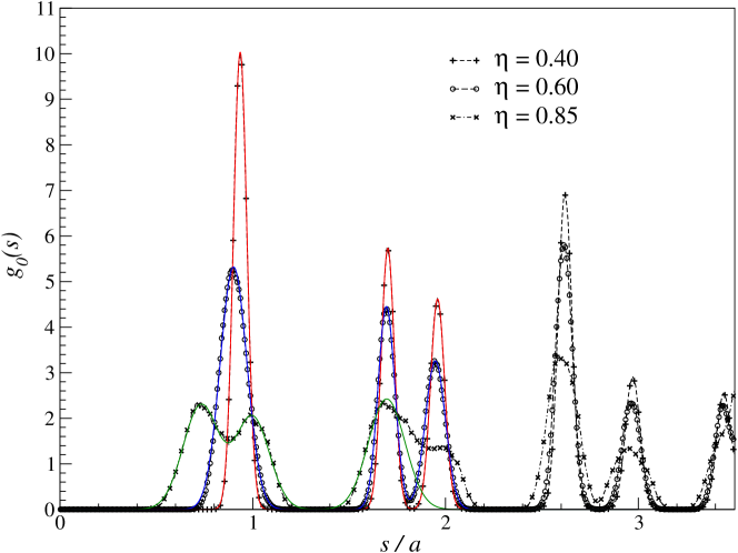
Figure 4: (colors online) Pair correlation function $g_{0}(s)$ (defined in the text), as a function of the in-plane distance $s$ (in units of $a$) between particle 0 and the particles in the monolayer. Results are shown for three different values of $\eta$, along the “out”-branch. Symbols: MC data; coloured lines: fits to the MC results using Equation (14) with $M_{p}=3$.

Since the coupling constant $\Gamma$ was chosen at a rather high value – $\Gamma\simeq 1550$ – the use of the harmonic approximation for the Wigner crystal is fully justified Ashcroft:book:76 . This allows to approximate the $M_{p}$ first peaks in the correlation functions as a sum of Gaussian functions:

$$g_{0}(s)=\sum_{n=1}^{M_{p}}G_{n}^{(0)}\exp\left(-\frac{(s-s_{n})^{2}}{2\lambda_{n}^{2}(\Gamma)}\right)\ ,$$ (14)

$s_{n}$ being the position of the $n$-th peak, $G_{n}^{(0)}$ its amplitude, and $\lambda_{n}(\Gamma)$ its width. Finally, the number of particles $N_{n}$ that populate the $n$-th shell (which is defined by the $n$-th peak) are computed via

$$N_{n}\,=\,2\pi\sigma\,G_{n}^{(0)}\int_{0}^{\infty}s\,\exp\left(-\frac{(s-s_{n})^{2}}{2\lambda_{n}^{2}(\Gamma)}\right)\,ds.$$ (15)

Examples for the correlation function $g_{0}(s)$ along the “out”-branch are shown for three representative $\eta$-values in Figure 4. After fitting by a sum of Gaussians – cf. Equation (14) – we can determine the (average) positions of the particles within the monolayer via the peak positions of the Gaussians; this information allows, finally, for an accurate determination of the location (and then the displacements) of the particles. The positions of the first three peaks, $s_{1}$, $s_{2}$, and $s_{3}$, of the correlation function $g_{0}(s)$, are shown in Figure 5 as functions of $\eta$. As expected, for $\eta\to 0$ where the tagged particle is part of the ideal 2D Wigner crystal, these three $s$-values tend to their ideal undistorted hexagonal lattice expressions. These results show that finite size effects are negligible, with very similar results for small ($N=256$) as well as larger ($N=2025$) systems.

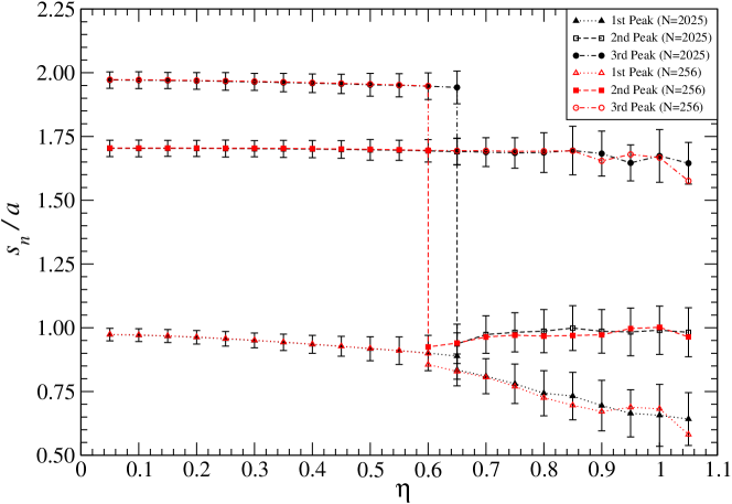
Figure 5: Positions of the first three peaks ($s_{1}$, $s_{2}$, $s_{3}$) of $g_{0}(s)$ (shown in Figure 4 for selected $\eta$-values) as functions of distance $\eta$, along the “out”-branch. These MC results are shown for two different system sizes. Lines are guides to the eye. The error bars are the width of the Gaussians, $\lambda_{n}$, defined in Equation (14); they are shown only for $N=2025$ particles since they are of comparable size for the 256 particle systems. For $\eta=0$ the following values of the ideal 2D Wigner crystal are quite well recovered: $s_{1}/a\simeq 1$, $s_{2}/a\simeq\sqrt{3}\simeq 1.73$ and $s_{3}/a\simeq 2$.

4 Analytic treatment

In this Section, we aim at calculating analytically the energy differences, $E^{\rm out}(\eta)$ and $E^{\rm in}(\eta)$ as defined in Equation (7), along the “out-” and the “in”-branches. For tractability, we assume that only the nearest neighbours of the reference particle 0 can leave their positions in the Wigner crystal, while the remaining particles are assumed to be fixed at their original positions in the lattice. For the “out”-branch, the rationale stems from Figure 5, showing that the second and third layers of neighbours are only weakly displaced by the polarisation effect of the reference particle. For the “out”-branch, this means that six particles are allowed to move as $\eta$ changes, while for the “in”-branch, there are only three charges (see below). We use a recently proposed analytic technique Samaj12a ; Samaj12b , which enables us to express lattice Coulomb summations in terms of quickly convergent series of the generalised Misra functions

$$z_{\nu}(x,y)=\int_{0}^{1/\pi}\frac{{\rm d}t}{t^{\nu}}{\rm e}^{-xt}{\rm e}^{-y/t},\qquad y>0.$$ (16)

4.1 “Out”-branch

The left panel of Figure 6 defines those six particles allowed to respond to the presence of the tagged particle (the projection of which yields the shaded disk). We have allowed – by introducing parameters $\delta$ and $\delta^{\prime}$ – the possibility of a symmetry breaking among neighbours. The hexagonal Wigner crystal is represented by black and white particles, as discussed above. The positions of the fixed black particles are given by vectors $a(j,\sqrt{3}k)$, where $j$ and $k$ are any two integers, except for the pairs $(j,k)=(0,0),(1,0),(-1,0)$, the latter two combinations corresponding to the black particles which are allowed to be displaced. The positions of the fixed white particles are given by vectors $a\left(j+\frac{1}{2},\sqrt{3}(k+\frac{1}{2})\right)$, where the pairs $(j,k)=(0,0),(-1,0),(0,-1),(-1,-1)$ are excluded.

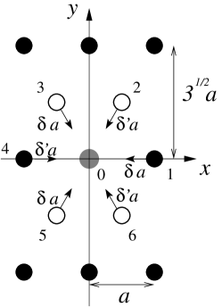
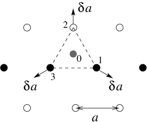
Figure 6: Approximations used for the analytic treatment. Left panel: along the “out”-branch, only the six labeled neighbours are allowed to leave their perfect lattice positions. Arrows indicate two possible, alternating displacements ($\delta a$ and $\delta^{\prime}a$). As compared to Figure 3, we have $\delta_{1}=\delta_{3}=\delta_{5}=\delta$ and $\delta_{2}=\delta_{4}=\delta_{6}=\delta^{\prime}$. Left panel: along the “in”-branch, only the three particles carrying indices 1 to 3 can move, along the arrows, when the tagged particle is approached. In both “in”- and “out”-cases, the displacements are radial.

The energy of the given particle configuration, $E^{\rm out}(\eta;\delta,\delta^{\prime})$, has the following four contributions:

• The interaction of particles labeled 1 to 6 with the remaining fixed particles and neutralising background:

  $$E_{1}(\delta,\delta^{\prime}) = 3\frac{e^{2}}{a}\Bigg{[}I(\delta,\sqrt{3})+J(\delta,\sqrt{3})+I(\delta^{\prime},\sqrt{3})+J(\delta^{\prime},\sqrt{3})$$ (17)

  $$-\frac{1}{1-\delta}-\frac{1}{2-\delta}-\frac{2}{\sqrt{1-\delta+\delta^{2}}}-\frac{2}{\sqrt{3-3\delta+\delta^{2}}}$$

  $$-\frac{1}{1-\delta^{\prime}}-\frac{1}{2-\delta^{\prime}}-\frac{2}{\sqrt{1-\delta^{\prime}+\delta^{\prime 2}}}-\frac{2}{\sqrt{3-3\delta^{\prime}+\delta^{\prime 2}}}\Bigg{]},$$

  where the definitions of the lattice sums $I(\delta,\Delta)$, $J(\delta,\Delta)$, and their series representations are given in Equations (27) and (28) of the Appendix, respectively. In practice, these series must be truncated at some finite value $M$, i.e. summed over the set $1,2,\ldots,M$ or $-M,-M+1,\ldots,M$. Since these series are quickly convergent, we have chosen here and in what follows a cutoff value of $M=5$, which reproduces the exact energy values to 17 decimal digits Samaj12b .

• The interaction of particles labeled 1 to 6 with each other:

  $$E_{2}(\delta,\delta^{\prime})=\frac{e^{2}}{a}\left[\frac{6}{\sqrt{1-\delta-\delta^{\prime}+\delta^{2}+{\delta^{\prime}}^{2}-\delta\delta^{\prime}}}+\frac{\sqrt{3}}{1-\delta}+\frac{\sqrt{3}}{1-\delta^{\prime}}+\frac{3}{2-\delta-\delta^{\prime}}\right].$$ (18)

• The interaction of the tagged particle 0 with the fixed charges in the remaining Wigner crystal and with the neutralising background

  $$E_{3}(\eta)=\frac{e^{2}}{a}\left[K(\eta)+L(\eta)-\frac{6}{\sqrt{1+\sqrt{3}\eta^{2}}}\right],$$ (19)

  where the lattice sums $K(\eta)$ and $L(\eta)$ are defined in Equations (30) and (31) of the Appendix, respectively.

• The interaction of the tagged particle $0$ with particles labeled 1 to 6:

  $$E_{4}(\eta;\delta,\delta^{\prime})=3\frac{e^{2}}{a}\left[\frac{1}{\sqrt{(1-\delta)^{2}+\sqrt{3}\eta^{2}}}+\frac{1}{\sqrt{(1-\delta^{\prime})^{2}+\sqrt{3}\eta^{2}}}\right].$$ (20)

The total energy shift is then given by

$$\delta E^{\rm out}(\eta;\delta,\delta^{\prime})=E^{\rm out}(\eta;\delta,\delta^{\prime})-E^{\rm out}(0;0,0),$$ (21)

where $E^{\rm out}(\eta;\delta,\delta^{\prime})=E_{1}(\delta,\delta^{\prime})+E_{2}(\delta,\delta^{\prime})+E_{3}(\eta)+E_{4}(\eta;\delta,\delta^{\prime})$. For a given value of $\eta$, the particle shifts $\delta$ and $\delta^{\prime}$ are determined by minimising $\delta E^{\rm out}(\eta;\delta,\delta^{\prime})$. Within the present approximation, where we assume that only six nearest neighbours are allowed to move, we obtain throughout $\delta=\delta^{\prime}$ irrespective of the value of $\eta$, i.e. symmetry breaking does not take place.

4.2 “In”-branch

To study the “in”-branch, we allow for the displacement of the three neighbours represented in the right panel of Figure 6. Assuming particle 3 to be located in the origin of the coordinate system, the $x$- and $y$-coordinates of the tagged particle are given by the vector ${\bm{s}}=a\left(1/2,\sqrt{3}/6\right)$. For a finite value of distance $\eta$, it is assumed that the positions of particles 1, 2 and 3 are shifted from their ideal positions by $\delta a$, in directions pointing away from particle 0. The remaining particles of the Wigner crystal are assumed to be fixed: black particles at positions $a(j,\sqrt{3}k)$, excluding integer pairs $(j,k)=(0,0),(1,0)$ and white particles at positions $a\left(j+\frac{1}{2},\sqrt{3}(k+\frac{1}{2})\right)$, with $(j,k)\neq(0,0)$; the aforementioned excluded pairs of indices correspond to the positions of the mobile particles.

The energy of the given particle configuration, $E^{\rm in}(\eta;\delta)$, bears the following four contributions:

• The interaction of particles labeled 1 to 3 with the remaining, fixed particles in the Wigner crystal and with the neutralising background:

  $$E^{\prime}_{1}(\delta)=3\frac{e^{2}}{a}\left\{\frac{1}{\sqrt{3}}\left[I\left(\frac{\delta}{\sqrt{3}},\frac{1}{\sqrt{3}}\right)+J\left(\frac{\delta}{\sqrt{3}},\frac{1}{\sqrt{3}}\right)\right]-\frac{2}{\sqrt{1+\sqrt{3}\delta+\delta^{2}}}\right\}.$$ (22)

• The interaction of particles labeled 1 to 3 with each other:

  $$E^{\prime}_{2}(\delta)=3\frac{e^{2}}{a}\frac{1}{1+\sqrt{3}\delta}.$$ (23)

• The interaction of the tagged particle 0 with the fixed charges in the remaining Wigner crystal and with the neutralising background:

  $$E^{\prime}_{3}(\eta)=\frac{e^{2}}{a}\left\{\frac{1}{2}\left[\sqrt{3}K(\sqrt{3}\eta)-K(\eta)+\sqrt{3}L(\sqrt{3}\eta)-L(\eta)\right]-\frac{3}{\sqrt{\frac{1}{3}+\sqrt{3}\eta^{2}}}\right\}.$$ (24)

• The interaction of the tagged particle 0 with particles labeled 1 to 6:

  $$E^{\prime}_{4}(\eta,\delta)=3\frac{e^{2}}{a}\frac{1}{\sqrt{\left(\frac{1}{\sqrt{3}}+\delta\right)^{2}+\sqrt{3}\eta^{2}}}.$$ (25)

Again, the lattice sums $I(\delta,\Delta)$, $J(\delta,\Delta)$, $K(\delta,\Delta)$, and $L(\delta,\Delta)$ are given in the Appendix in Equations (27), (28), (30), and (31).

The total shift in energy is then given by

$$\delta E^{\rm in}(\eta,\delta)=E^{\prime}_{1}(\delta)+E^{\prime}_{2}(\delta)+E^{\prime}_{3}(\eta)+E^{\prime}_{4}(\eta,\delta)+\frac{e^{2}}{a}\left(3-\frac{15}{\sqrt{2}3^{1/4}}c\right),$$ (26)

where the last (constant) term is determined by the asymptotic condition (10). As before, the particle shift $\delta$ is determined by minimising $\delta E^{\rm in}(\eta,\delta)$.

5 Results

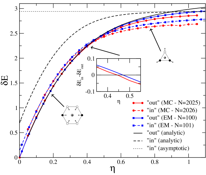
Figure 7: (colors online) Excess system energy $\delta E$ with respect to the undistorted Wigner crystal, in units of $e^{2}\sqrt{\sigma}$. Red, blue, and black lines are respectively for Monte Carlo (MC), energy minimisation (EM), and analytic results. The full lines display the “out”-branch data, while the broken ones are for the “in”-branch. Horizontal dotted line: prediction of Equation (10) for the asymptotic energy along the “in”-branch, $\delta E(\eta\to\infty)/(e^{2}\sqrt{\sigma})=-3c/2\simeq 2.94077$. The inset shows the difference between “’in”- and “out”-energies, for both MC and EM.

The central object in our study is the total Coulombic energy of the system (“monolayer + tagged charge”), suitably shifted by its value at $d=0$ to obtain a well behaved quantity for large systems (with $N\gg 1$). Figure 7 therefore conveys our main results, showing $\delta E^{\rm in}(\eta)$ and $\delta E^{\rm out}(\eta)$, as defined in Equation (7), calculated via the two numerical approaches as well as with the analytic method. First of all, the three methods display very consistent results on the “out”-branch. Only for large $\eta$ do they start to depart, with the analytical prediction providing expectedly higher energy configurations. This clearly stems from the assumption that only the six labeled charges in the left panel of Figure 6 are mobile. Turning to the “in”-branch, we observe that restricting the mobile charges to now a set of three (see Section 4), becomes more problematic. The analytical “in”-branch energy departs significantly from the results of energy minimisation and MC, the latter two being again consistent (broken lines). We note that the limiting cases discussed in Section 2.2 are obeyed. The energy graph is indeed compatible with the “in”-bound (10). In addition, we can extrapolate from the data that $\delta E^{\rm out}(\infty)>\delta E^{\rm in}(\infty)$, as a fingerprint of metastability along the “out”-branch, even at large $\eta$. On the other hand, at short distances, a related metastable blocking is observed for the “in”-branch, resulting in values of $\delta E^{\rm in}(0)$ that are slightly positive.

Within a good agreement between the two numerical methods, the “in”- and “’out”-curves cross at $\eta_{t}\sim 0.47$, see also the inset of Figure 7. Thus, below this value, the stable state lies on the “out”-branch, while for $\eta\gtrsim 0.47$, the “in”-branch structure is energetically more favourable. What are the configurations of the charges along these two branches? In particular, is coordination six retained along the “out”-protocol, and likewise is coordination three retained all along the “in”-branch? To answer these questions, we will focus on the particle displacements. Even though the “out”- and the “in”-branches are metastable for $\eta\gtrsim 0.47$ and for $\eta\lesssim 0.47$, respectively, we will discuss some of their properties not only for stable but also for metastable particle configurations, as we have observed some interesting features.

The displacement of the six most central particles ($\delta_{1}$ to $\delta_{6}$), as calculated along the “out”-branch, are accumulated in Figure 8 as functions of $\eta$. They are computed from the particle positions at $\eta=0$, indicated by the peaks of the corresponding $g_{0}(s)$. For $0\leq\eta\lesssim 0.63$, $\delta_{i}$-values ($i=1,\cdots,6$) are all positive and equal: upon increasing $\eta$, the ring of inner particles contracts uniformly towards the vacancy, while fully maintaining the six-fold rotational symmetry of the particle arrangement (see left-most schematic inset in Figure 8). However, when passing this $\eta$-threshold value, symmetry breaking takes place: for $0.63\lesssim\eta\lesssim 0.85$, the particle configuration has now only three-fold rotational symmetry. The six most central particles split up into two sets of three: (i) particles of the first set (say 1, 3, 5), with their $\delta_{i}$-values being throughout positive, have shifted towards positions that are closer to the vacancy than the positions of the second set; (ii) the displacements of the particles of the latter set (say 2, 4, 6) decrease in this $\eta$-range monotonously; they even become negative at $\eta\simeq 0.7$, indicating that for $\eta\gtrsim 0.70$ particles of the second set are more distant from the vacancy than in the ideal Wigner crystal. At this point it should be noted, that the best and the second-best configurations as determined via energy minimisation often differ by minute differences in their energy (i.e., by a few tenth or less of a percent).

On the other hand, the analytical treatment does not predict this very scenario, even if it a priori allows for a symmetry breakdown of the type “3 + 3” (see Figure 6). This points to the subtle effect of charge displacement beyond the first ring of neighbours, which although small, can influence the structure in a non-trivial way. We emphasise at this point the excellent agreement between data obtained from the energy minimisation approach and results extracted from MC simulations, that extends for distances of the tagged particle up to $\eta\simeq 0.85$. Finally, as we pass this $\eta$-value, another transition takes place to a configuration with only two-fold symmetry (see the right-most particle sketch of Figure 8): two sets of particles form with two particles (say, indices 1 and 4), the other one with four particles (say, indices 2, 3, 5, and 6). According to the minimisation approach, this transition is discontinuous, while there are indications that in MC simulations, this transition is continuous; due to the large error bars (see discussion below) an unambiguous conclusion about the nature of this transition is difficult to reach. For the former set of particles (where the two charges are located on opposite positions with respect to the vacancy), the $\delta$-values are positive. The charges thus have approached the hole left by the tagged particle. The other four charges (forming the second set) are characterised by small, negative $\delta$-values (which, with increasing $\eta$, tend to zero), indicating that these particles have moved away from the central position of the vacancy.

At this point it is worthwhile to note that – while the average values for the displacement as computed via MC simulations are in close agreement with the data obtained with the energy minimisation approach (and with the analytical results for $\eta\lesssim 0.65$) – the fluctuations of the MC-data are non-negligible. To be more specific, for $\eta\lesssim 0.6$, the agreement between the two sets of numerical data is better than 1% and at most 3 to 5 % for higher $\eta$-values (see data shown in Figure 8). However, the error bars, given by the respective $\lambda_{n}$-values and displayed in this figure are quite large, and do increase when $\eta$ increases. This is due to the fact that particles in the layer are pinned by the external potential of the reference charge, which becomes softer as $\eta$ grows. The resulting fluctuations ensure that the MC algorithm explores thoroughly the phase space “around” the equilibrium positions; it is the excellent accuracy of the harmonic approximation that is able to identify well the equilibrium positions of the particles as compared with the positions obtained via the energy minimisation approach and via the analytic method. A similar analysis can be applied to the energy curves shown in Figure 7.

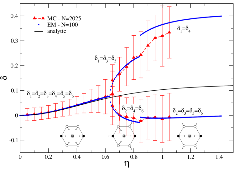
Figure 8: (colors online) Deformations $\delta_{1}$ to $\delta_{6}$ (in units of $a$) of the six nearest neighbours of the tagged particle along the “out”-branch as defined in the left panel of Figure 3 as functions of $\eta$. Blue dots: results from the energy minimisation approach, black line: results from the analytic approach. Red symbols: deformations calculated from the positions of the first peak in $g_{0}(s)$; broken red line is drawn as a guide to the eye. Error bars indicate the $\sigma$-values of the Gaussian fit – cf. Equation (14). The three schematic views provide a qualitative impression of the displacement of the six, most central particles.

We now proceed with a more quantitative analysis of the aforementioned splitting of the six most central particles in two subsets of charges. This fact is visible in the $s_{1}$-branch shown in Figure 5, and also appears in the bottom panel of Figure 9. The other two branches of Figure 5 (displaying data for $s_{2}$ and $s_{3}$) show a weak, monotonous decrease with increasing $\eta$, indicating that not only the nearest neighbours are affected by the displacement of the tagged particle, but also second and third nearest neighbours (even though their displacements are much weaker). Finally, the top panel of Figure 9 provides evidence that the number of particles in each shell assumes an essentially constant and $\eta$-independent value of six (deviations for $\eta\gtrsim 0.7$ can be attributed to the statistical noise in MC simulations). We conclude that the perturbation induced by the tagged charge progresses shell-by-shell throughout the crystal.

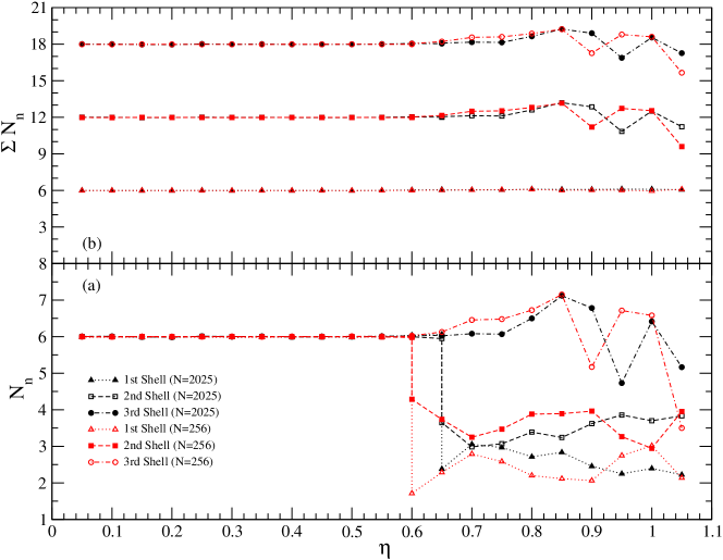
Figure 9: MC simulations along the “out”-branch. Bottom panel: number of neighbours, $N_{n}$, in the first three shells ($n=1,2,3$) as functions of $\eta$. Top panel: sum over the neighbours located within the first, the second, and the third shell, as functions of $\eta$. Results are shown for two different system sizes, lines are drawn as guide to the eye.

To complete our discussion on the displacement of the particles, we turn to the “in”-branch: here the scenario is simpler since three-fold symmetry is maintained along the entire branch, with the $\delta$-values decreasing continuously, to vanish at large $\eta$. Since the analytical prediction is less reliable here, as explained earlier, less effort was devoted to studying that branch. Only nearest neighbour results from MC simulations are shown, since the localisation of charges is less accurate for the next nearest neighbours (i.e., $\delta^{\prime}$ data). It can be seen in Figure 10 that the trend found in MC, EM and analytically is consistent, and that the small differences between the two numerical data sets do not alter the good agreement found at the level of the energy, see Figure 7. The energy minimimization route allows for an accurate determination of the individual displacements $\delta$ and $\delta^{\prime}$ of each of the labeled particles in the right panel of Figure 3; we find that particles carrying labels 1, 2, and 3 are displaced (within numerical accuracy) by the same displacement $\delta a$, while the other three particles (with indices 4, 5, and 6) are shifted by the same $\delta^{\prime}a$-value. Thus we can conclude that throughout the entire “in”-branch three-fold coordination is preserved.

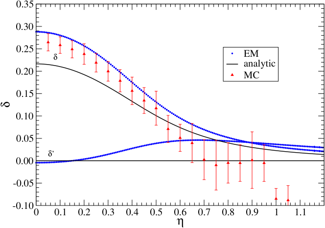
Figure 10: Same as Figure 8, along the “in”-branch. The displacements (defined in the right panel of Figure 3) are computed from the positions occupied at large $\eta$. The energy minimisation (EM) was performed on a system with $N=101$ particles, while $N=2026$ in MC.

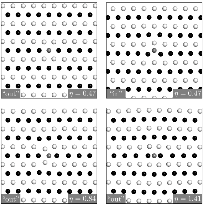
Figure 11: Particle arrangements induced by the tagged charge (the projection of which is shown in grey, as in previous graphs). Top panels: the two competing configurations at the transition point $\eta_{t}\simeq 0.47$ (“in” and “out” branches). Bottom panels: two “out”-branch configurations in the metastable region.

Finally, in an effort to provide a quantitative impression about the influence of the tagged particle on the displacement of the charges in the monolayer, we have collected in Figure 11 views of particle arrangements for selected $\eta$-values. In addition, we have concatenated sequences of equilibrium configurations for increasing (“out”-branch) and decreasing (“in”-branch) $\eta$-values into short animations, which are presented in the Supplementary Material. It can be seen in Fig. 11 that at the transition point $\eta_{t}$, the like-energy configurations associated to the two branches are quite distinct, and in addition do not exhibit significant displacements from their respective reference state ($d=0$ perfect hexagonal structure in the “out” case, and $d\to\infty$ perfect structure in the “in” case, see Section 2.2). The polarisation effect of the reference particle is thus quite weak here, an information already conveyed in Figs. 8 and 10. The bottom panel of Fig. 11 illustrates the symmetry breakdown phenomenon which arises, along the “out” branch, for $\eta>0.63$. The coordination number, which has a value of six for $\eta<0.63$, decays to three (as is seen for $\eta=0.84$), and ultimately to two for larger distances ($\eta=1.41$).

6 Conclusion

We have investigated how a 2D Wigner crystal formed by charges can be polarised, at $T=0$, by a single tagged charge. Starting from a perfect crystal on a planar neutralising background, we take off one reference charge from its equilibrium position, and fix it at a given distance $d$. This creates a vacancy in the plane, towards which some of the other charges move. For all $d$ values, we have determined the ground-state properties and structure of the system. Starting from the expected ground-states at $d=0$ and $d\to\infty$ respectively, we followed the particle rearrangements along the corresponding “out”- and “in”-branches, evidencing the metastability of the system. Two numerical techniques were used, namely direct energy minimisation and Monte Carlo simulations at a sufficiently small temperature. A third, independent procedure, of the evolutionary type, was also employed to check some of the results. In addition, an analytic treatment was performed, under the assumption that only those neighbours that are closest to the tagged particle (in either the $d=0$ or the $d\to\infty$ case) are allowed to move: thus six along the “out”-branch, and three along the “in”-one. All point charges interact through the usual $1/r$ potential, which requires careful numerical treatment, and use of recently derived results for handling lattice summations with extremely high precision. Since all particles bear the same charge and our interest is focused on ground-state features, the results obtained are independent of the value of the charge.

We proved the existence of a transition distance $d_{t}\simeq 0.47\sqrt{2/\sigma}$, $\sigma$ being the background density, so that for $d<d_{t}$, the reference charge is six-fold coordinated, while for $d>d_{t}$, the coordination is three. In terms of lattice spacing $a$, the transition distance reads $d_{t}\simeq 3^{1/4}\,0.47a\simeq 0.62\,a$. The transition between both states is discontinuous, and involves an energy barrier that has not been investigated in this contribution. The actual evaluation of the height of this barrier would require different tools than the ones used in this paper; we have therefore postponed this undoubtedly interesting question to a future contribution. One can assume (or anticipate) that this barrier is sufficiently high so that once the system lies on a given branch (“in” or “out”), it stays trapped in the corresponding energy valley: the “out”-branch was observed to be metastable for $d>d_{t}$, and conversely, the “in”-branch is metastable for $d<d_{t}$. While the “out”-branch state is of coordination six in its range of stability, a symmetry breaking takes place around $d\simeq 0.63\sqrt{2/\sigma}$, beyond which the “out”-branch is three-fold, and ultimately, two-fold coordinated.

As far as the “out”-branch is concerned, good agreement between the numerical and analytical results was reported. The situation complicates for the “in”-branch. First of all, the exact treatment assumed a priori in that case only three mobile neighbours, a number which turned out to be insufficient. Allowing for more mobile neighbours (say six, as for the “out”-analysis), would certainly improve the predictions. In addition, the “in”-case is also more elusive within the MC scheme. The reference state is indeed the large $d$ case, where the coupling energy between the fixed reference charge and the monolayer becomes small, and is washed out by the fluctuations induced by temperature. A more refined study of the “in”-branch is left for the future.

An interesting question, coupled to that of the energy barrier alluded to above, pertains to the structure of the transition state (the one at the saddle point between the two states at $d_{t}$). It is left for future investigations.

Appendix A Series representations of lattice sums

The lattice sums for the energies (17), (22), and their series representations in terms of the generalized Misra functions (16), read as

$$I(\delta,\Delta) = \sum_{(j,k)\neq(0,0)}\frac{1}{\sqrt{(j+\delta)^{2}+\Delta^{2}k^{2}}}-\mbox{backgr}=-\frac{4}{\sqrt{\Delta}}+\frac{1}{\sqrt{\pi\Delta}}$$ (27)

$$\times\Bigg{\{}2\sum_{j=1}^{\infty}\cos(2\pi j\delta)z_{3/2}(0,j^{2}\Delta)+2\sum_{j=1}^{\infty}z_{3/2}(0,j^{2}/\Delta)$$

$$+4\sum_{j,k=1}^{\infty}\cos(2\pi j\delta)z_{3/2}(0,j^{2}\Delta+k^{2}/\Delta)+\sum_{j=-\infty}^{\infty}z_{3/2}(0,(j+\delta)^{2}/\Delta)$$

$$-\frac{\sqrt{\pi\Delta}}{\delta}+2\sqrt{\pi}+2\sum_{j=1}^{\infty}\sum_{k=-\infty}^{\infty}z_{3/2}(0,j^{2}\Delta+(k+\delta)^{2}/\Delta)\Bigg{\}}$$

$$J(\delta,\Delta) = \sum_{(j,k)\neq(0,0)}\frac{1}{\sqrt{(j+\frac{1}{2}+\delta)^{2}+\Delta^{2}(k+\frac{1}{2})^{2}}}-\mbox{backgr}=-\frac{2}{\sqrt{\Delta}}+\frac{1}{\sqrt{\pi\Delta}}$$ (28)

$$\times\Bigg{\{}2\sum_{j=1}^{\infty}(-1)^{j}\cos(2\pi j\delta)z_{3/2}(0,j^{2}\Delta)+2\sum_{j=1}^{\infty}(-1)^{j}z_{3/2}(0,j^{2}/\Delta)$$

$$+4\sum_{j,k=1}^{\infty}(-1)^{j+k}\cos(2\pi j\delta)z_{3/2}(0,j^{2}\Delta+k^{2}/\Delta)$$

$$+2\sum_{j=1}^{\infty}\sum_{k=-\infty}^{\infty}z_{3/2}(0,(j-\textstyle{\frac{1}{2}})^{2}\Delta+(k-\textstyle{\frac{1}{2}}+\delta)^{2}/\Delta)\Bigg{\}}.$$

The expression in (27) is finite also in the limit $\delta\to 0$, due to the fact that

$$z_{3/2}(0,\delta^{2}/\Delta)\mathop{\sim}_{\delta\to 0}\frac{\sqrt{\pi\Delta}}{\delta}-2\sqrt{\pi}+O(\delta).$$ (29)

The lattice sums for the energies (19) and (24) are given by

$$K(\eta) = \sum_{(j,k)\neq(0,0)}\frac{1}{\sqrt{j^{2}+3k^{2}+\sqrt{3}\eta^{2}}}-\mbox{backgr}$$ (30)

$$= \frac{1}{\sqrt{\pi}3^{1/4}}\left[I_{3}((\pi\eta)^{2},0)+I_{3}(0,\eta^{2})\right],$$

$$L(\eta) = \sum_{(j,k)}\frac{1}{\sqrt{(j+\frac{1}{2})^{2}+3(k+\frac{1}{2})^{2}+\sqrt{3}\eta^{2}}}-\mbox{backgr}$$ (31)

$$= \frac{1}{\sqrt{\pi}3^{1/4}}\left[I_{2}((\pi\eta)^{2},0)+I_{4}(0,\eta^{2})\right].$$

The definitions of the integrals over the Jacobi theta functions $I_{2}$, $I_{3}$ and $I_{4}$ are presented respectively in Equations (61), (62) and (63) of Ref. Samaj12b .

References

- (1) E.P. Wigner, Phys. Rev. 46, 1002 (1934).
- (2) R.S. Crandall and R. Williams, Phys. Lett. A 34, 404 (1971).
- (3) A.V. Chaplik, Sov. Phys. JETP 35, 395 (1972).
- (4) C.C. Grimes and G. Adams, Phys. Rev. Lett. 42, 795 (1979).
- (5) E.Y. Andrei, G. Deville, D.C. Glattli and F.I.B. Williams, Phys. Rev. Lett. 60, 2765 (1988).
- (6) T.B. Mitchell, J.J. Bollinger, D.H.E. Dubin, et al., Science, 282, 1290 (1998); Phys. Plasmas 6, 1751 (1999).
- (7) M. Bonitz, P. Ludwig, H. Baumgartner et al., Phys. Plasmas 15, 055704 (2008).
- (8) Yu.P. Monarkha and V.E. Syvokon, Low Temp. Phys. 38, 1067 (2012).
- (9) Y. Monarkha and K. Kono, Two-Dimensional Coulomb Liquids and Solids - Springer Series in Solid-State Science 142 (Springer, Berlin - 2004).
- (10) P.M. Platzman and H. Fukuyama, Phys. Rev. B 10, 3150 (1974).
- (11) L. Bonsall and A.A. Maradudin, Phys. Rev. B 15, 1959 (1977).
- (12) D.S. Fisher, B.I. Halperin and R. Morf, Phys. Rev. B 20, 4692 (1979).
- (13) J.M. Kosterlitz and D.J. Thouless, J. Phys. C 6, 1181 (1973).
- (14) D.R. Nelson and B.I. Halperin, Phys. Rev. B 19, 2457 (1979).
- (15) R. Messina, C. Holm and K. Kremer, Phys. Rev. E, 64, 021405 (2001).
- (16) R. Messina, J. Phys.: Condens. Matter 21, 113102 (2009).
- (17) V.M. Bedanov and F.M. Peeters, Phys. Rev. B 49, 2667 (1994).
- (18) M. Kong, B. Partoens and F.M. Peeters, Phys. Rev. E 67, 021608 (2003).
- (19) A. Libál, C. Reichhardt and C.J. Olson Reichhardt, Phys. Rev. E 75, 011403 (2007).
- (20) B. He and Y. Chen, Solid State Commun. 159, 60 (2013).
- (21) W. Lechner and Ch. Dellago, Soft Matter 5, 2752 (2009).
- (22) S. van Teeffelen, C.V. Achim and H. Löwen, Phys. Rev. E 87, 022306 (2013).
- (23) R.R. Netz, Eur. Phys. J. E 5, 557 (2001).
- (24) L. Šamaj and E. Trizac, Phys. Rev. Lett. 106, 078301 (2011).
- (25) A. Pertsinidis and X.S. Ling, Nature 413, 147 (2001).
- (26) A. Pertsinidis and X.S. Ling, Phys. Rev. Lett. 87, 098303 (2001).
- (27) M. Mazars, Phys. Rep. 500, 43 (2011).
- (28) R.H. Byrd, P. Lu, J. Nocedal, and C. Zhu, SIAM J. of Scient. Comp. 16, 1190 (1995).
- (29) J.H. Holland, Adaptation in Natural and Artificial Systems (The University of Michigan Press, Ann Arbor, 1975).
- (30) D. Gottwald, G. Kahl, and C. Likos, J. Chem. Phys. 122, 204503 (2005).
- (31) G. Doppelbauer, E. Bianchi, and G. Kahl, J. Phys.: Cond. Matt., 22, 104105 (2010).
- (32) M. Antlanger and G. Kahl, Cond. Matter Phys. 16, 43501 (2013).
- (33) M.E.J. Newman and G.T. Barkema, Monte Carlo Methods in Statistical Physics. (Oxford University Press - 1999).
- (34) M. Mazars, Mol. Phys. 103, 1241 (2005).
- (35) J.-J. Weis, D. Levesque and S. Jorge, Phys. Rev. B 63, 045308 (2001).
- (36) M. Mazars, EPL 84, 55002 (2008).
- (37) B.K. Clark, M. Casula and D.M. Ceperley Phys. Rev. Lett., 103, 055701 (2009).
- (38) N.W. Ashcroft and N.D. Mermin, Solid State Physics (Brooks/Cole, Thomson Learning - 1976).
- (39) L. Šamaj and E. Trizac, EPL 98, 36004 (2012).
- (40) L. Šamaj and E. Trizac, Phys. Rev. B 85, 205131 (2012).